1. Introduction
Systematic errors (biases) in precipitation measurements are commonly accounted for by means of correction models that can be expressed in the general form
where
is the corrected figure,
is the gauge-measured precipitation,
is the sum of correction terms for various error sources, and
is the wind deformation coefficient. The detailed model, originally proposed by [
1], was later modified by [
2] to account for both liquid and solid precipitation and can be written as
where
,
and
are the correction terms for wetting, evaporation, and mechanical errors, respectively, while subscripts
r and
s refer to liquid (rain) and solid (snow) precipitation (see also [
3]). This formulation reveals that the adjustment of catching (environmental) biases due to the wind applies to the precipitation amount once this is corrected for counting (instrumental) biases. The adjustment factor
is reportedly a function of the wind speed and precipitation intensity, and its value ranges between 1.0 and 1.15 for rain and between 1.0 and 2.0 for snow measurements [
4].
The correction of precipitation measurement biases is applied to daily or monthly totals or, in some practices, to individual precipitation events [
3]. However, since the precipitation intensity and the wind velocity are among the influencing variables, the most relevant sources of error act at very short to instantaneous timescales, at which point such factors may vary significantly. Corrections are often non-linear functions; therefore, it is important to develop correction algorithms that can be easily applied at the minimum temporal resolution of operational measurements (e.g., one-minute for rainfall intensity, as recommended by [
3]).
The influence of wind on precipitation measurements is due to the interaction between the gauge body and the airflow. Any precipitation gauge behaves as a bluff-body when impacted by wind, and this interaction produces airflow deformations around the obstacle. Generally, upward velocity components arise upwind of the collector and wind accelerates above it [
5,
6]. This aerodynamic effect deflects the hydrometeors (liquid/solid particles) with respect to their undisturbed trajectories [
4,
7], and is responsible for a significant reduction in the collection performance. The main factors of influence are the gauge geometry, the wind speed, and the type of precipitation (liquid or solid) and its characteristics, including the crystal type, Particle Size Distribution (
PSD) and precipitation intensity [
8,
9].
The problem of the wind-induced bias on precipitation measurements is addressed in the literature using both numerical simulation (Computational Fluid Dynamics (CFD) and particle tracking) and experiments (field and wind tunnel tests). Generally, wind produces underestimation in precipitation measurements, except for gauges with peculiar shapes (e.g., the Hotplate
© precipitation gauge, see [
10]). Reference [
1] reported that the typical magnitude of the wind–induced losses (undercatch) for the precipitation amount is 2–10% in case of liquid precipitation and 10–50% in case of solid precipitation. Field studies focusing on solid precipitation [
9,
11] showed collection losses up to 70–80%, while [
12] reported an observed undercatch of about 10 to 23% for liquid precipitation at a lowland and upland site, respectively. Nevertheless, the implementation of adjustments based on correction curves in operational conditions is still uncommon.
The drawbacks of adjustment functions derived from field experiments alone are related to their strict dependence on the site where the test field is geographically located, the associated precipitation and wind climatology, and on the reliability and accuracy of the assumed reference gauge. The observed Collection Efficiency (CE) values derive from the actual drop size distribution of precipitation events and the microphysical characteristics of the hydrometeors. Complete parameterization of these CE curves is rarely achieved, so that a large dispersion of the field-measured data around the best-fit curves usually persists.
It is evident that a theoretically based approach is needed, though still based on real-world observations for proper validation of the algorithms and results, to achieve a complete coverage of various local climatological characteristics, precipitation microphysics, gauge shapes and wind conditions. This can be achieved by exploiting the potential of numerically solving the basic equations of fluid motion and of particle-fluid interactions, as in our proposed method. In the present work, we base our study on CFD simulations already performed by [
13] for a cylindrical gauge which has the shape of the most widely used precipitation gauges.
With the aim of reducing the dispersion of field data around experimentally derived adjustment curves, and shedding light on the dependence of such curves on the drop size distribution and its link with the precipitation intensity, [
14] recently showed that such dispersion can be reduced by including the results of the numerical simulation into the best-fit methodology applied on field measurements. The authors analysed WMO-SPICE quality controlled 30-min accumulation data from the Marshall field-test site (CO, USA) and revealed that the wind-induced undercatch of precipitation gauges is best correlated with the measured precipitation intensity, rather than temperature (widely used, e.g., in [
15]), in addition to wind speed. The measured precipitation intensity indeed has the advantage of including information about the particle size distribution [
16]. The optimal curve fitting used by [
14] to derive adjustment curves for the Geonor
© T200B gauge in a Single Alter shield and in a reference configuration indicated that accounting for precipitation intensity indeed reduces the scatter of the residuals. This result is confirmed by the analysis of data from other field test sites, such as CARE (Canada) and Haukeliseter (Norway), and shows consistent behaviour under different climatological conditions.
The physical basis for the improved parameterisation of the adjustment curves obtained by using the measured precipitation intensity was shown to derive from the correlation of large particles with high intensities. Large particles are preferentially collected by the gauge, even in strong wind, due to their higher fall velocity, allowing them to break through streamlines of flow above the gauge. The numerical modelling was able to reproduce the collection efficiency pattern observed in the field. The authors’ findings provide an attractive method to improve operational measurements, since no additional instrument, except for a wind sensor, is required to derive the adjusted estimates of snow accumulation.
In the present work, the formulation of CE curves as a function of wind speed () is derived for a typical cylindrical gauge and parameterized with the Rainfall Intensity (RI). Easy-to-use adjustment curves are finally obtained as a function of the rainfall intensity measured by the gauge (RImeas) and wind speed.
Existing Correction Algorithms
Adjustment curves can be derived using data from experimental sites equipped with different precipitation gauges in operational conditions, and a reference one. In field studies, the ratio between the precipitation measured by a gauge in operational conditions,
(usually in (mm)) for a given wind speed,
(m s
−1) and the reference one,
(mm) is called the Collection Efficiency (
CE)
The World Meteorological Organization (WMO) recommends using a gauge placed in a pit as the reference instrumental configuration for liquid precipitation, with the gauge orifice at ground level, sufficiently distant from the nearest edge of the pit to avoid in-splashing. A strong plastic or metal anti-splash grid with a central opening for the gauge must cover the pit, except for the central opening where the gauge orifice is located (construction details are provided in [
17]). Because of the absence (or very limited effect) of wind-induced bias, pit gauges generally report more precipitation than any elevated gauge.
The reference installation for solid precipitation is known as the Double Fence Intercomparison Reference (DFIR) [
18]. It has octagonal vertical double fences surrounding a storage or automatic gauge, which itself is equipped with a Single Alter shield. Note that this reference configuration is not free from measurement biases itself, and its construction could be improved [
19].
At an experimental site in Haukeliseter (Norway), two Geonor
© T200B weighing gauges, in unshielded and single Alter shielded configurations, were installed close to the DFIR. Temperature measurements were also available, and anemometers were located at the height of ten meters and at the gauge collector height. The authors classified the precipitation in solid, mixed, or liquid [
15], according to the air temperature thresholds reported by [
20]. For temperatures
T < −2 °C the precipitation is mainly falling as snow, and the
CE has a characteristic fast decreasing behavior with the wind speed. For
T > 2 °C, where the precipitation is mainly falling as rain, the
CE is less influenced by the wind. Rain, snow and mixed precipitation occur in the range −2 °C ≤
T ≤ 2 °C, and a larger scatter appears depending on the precipitation type. Based on a three-year dataset from the Haukeliseter test site, containing several concurrent observations of the
CE, the following adjustment curve was formulated by [
15]
where
and
are two fitting parameters,
is the temperature threshold and defines the transition between the two limits above, while
indicates the fuzziness between rain and snow, and
is a parameter governing the variance in the measurement error.
The equation was obtained starting from the assumption that
CE is a function of wind speed and air temperature, in the form
the parameter
goes from one limit, dry snow, to another, mixed precipitation, when the temperature increases/decreases. A sigmoid function reasonably fits experimental data yielding the parametric function as follows
Application of the adjustment curve yields some residual differences between the adjusted accumulation and the reference one, which are probably ascribable to the actual (unknown) particle size distribution.
Data from winter 2010 in the two experimental sites of Marshall (USA) and Haukeliseter (Norway) were analysed by [
21]. The authors proposed the following exponential shape for
CE
where the experimental parameters
,
and
vary with the height of the anemometer and the type of precipitation gauge (unshielded, Single Alter shielded, etc.). After correction, a significant scatter of data persists, which is probably due to the effect of noise, the spatial variability of precipitation and also the spatial variability in crystal type, that are not fully taken into account in this study. With the aim of deriving adjustment curves that could be extended to other sites, data from eight experimental sites were further analysed by [
22]. The study provided the parameters of Equation (7) for Single Alter shielded and unshielded chimney shaped weighing gauges, by separating mixed and solid precipitation, and for wind speed measured at ten meters or at the collector elevation.
The dataset obtained by [
23] at the Formigal (Spain) experimental site was divided into two samples, and adjustment curves were derived for tipping-bucket rain gauges at one- and three-hours accumulation. For one-hour accumulation, the authors propose Equation (8), where a contribution of the melting of snow during the previous hour of accumulation is also included
where
is the adjusted hourly precipitation,
is the measured one, and
is the cumulated precipitation in the previous hour.
2. Method
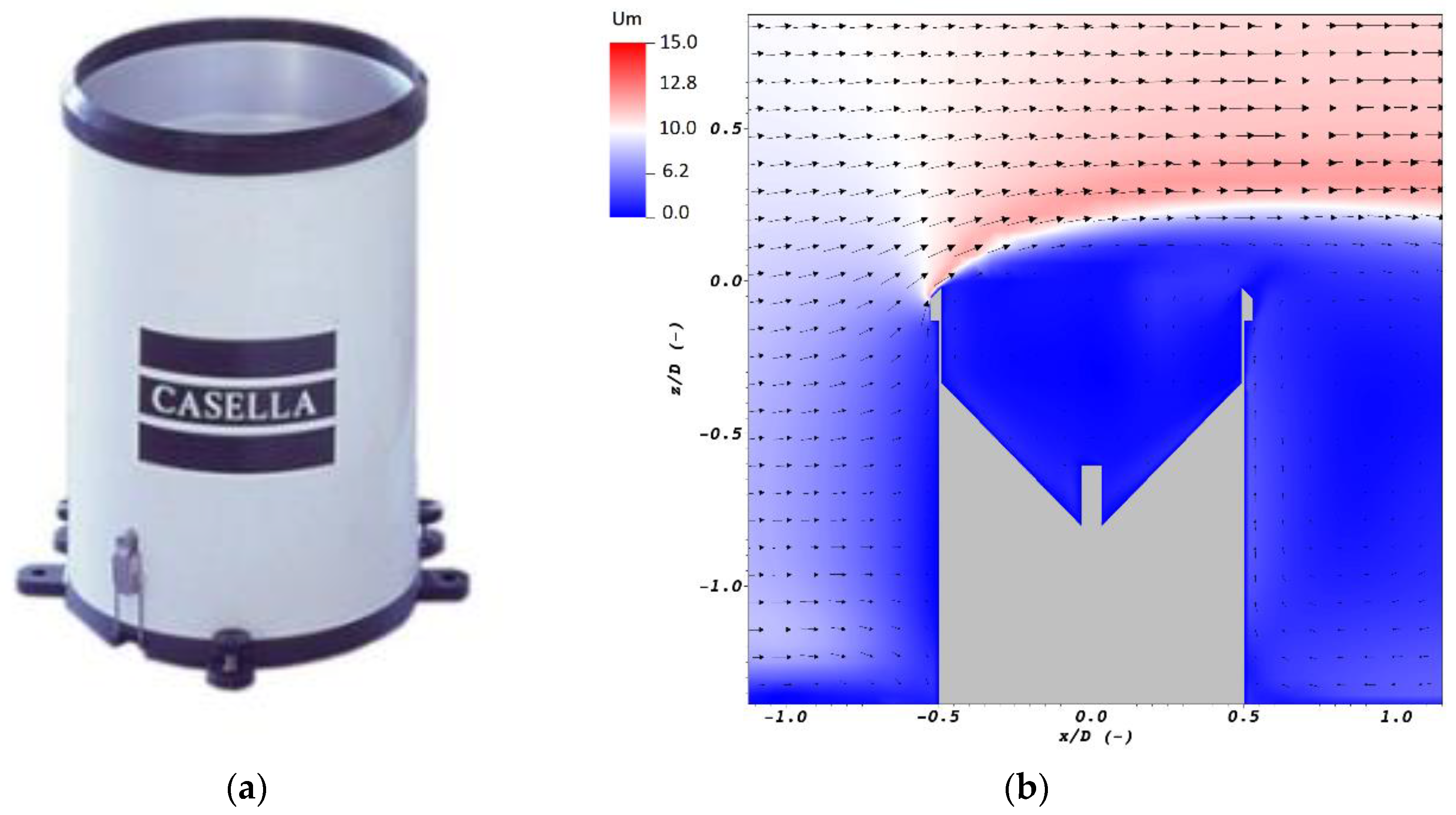
In the present work, the airflow field (velocity magnitude and components) around a cylindrical gauge, the Casella
© tipping-bucket gauge (hereinafter Casella, see
Figure 1), was adopted to simulate the trajectories of water drops and to calculate the
CE based on a suitable
PSD. We started from the CFD simulations (see
Figure 1) partially published in the work of [
13] for various wind speeds (
= 2, 5, 7, 10, and 18 m s
−1).
The Lagrangian Particle Tracking (LPT) model used by [
9] for solid precipitation was modified by [
24] to introduce drag coefficient equations suitable for liquid precipitation. These were derived for various ranges of the particle Reynolds number among those proposed in the literature by [
7], and formulated starting from data published by [
25,
26]. Drop trajectories are computed from the particle motion equation, by calculating, at short time intervals, the particle position, velocity, and acceleration. The relative particle-to-air velocity is updated at every time step by interpolating the CFD airflow field to obtain the flow velocity in the exact position of the drop. Water drops are assumed to be spherical, with the associated equivalent diameter
d, while the density of liquid water was set as equal to 1000 kg m
−3 at the air temperature of 20 °C. This model was validated by means of a dedicated wind tunnel campaign in [
24].
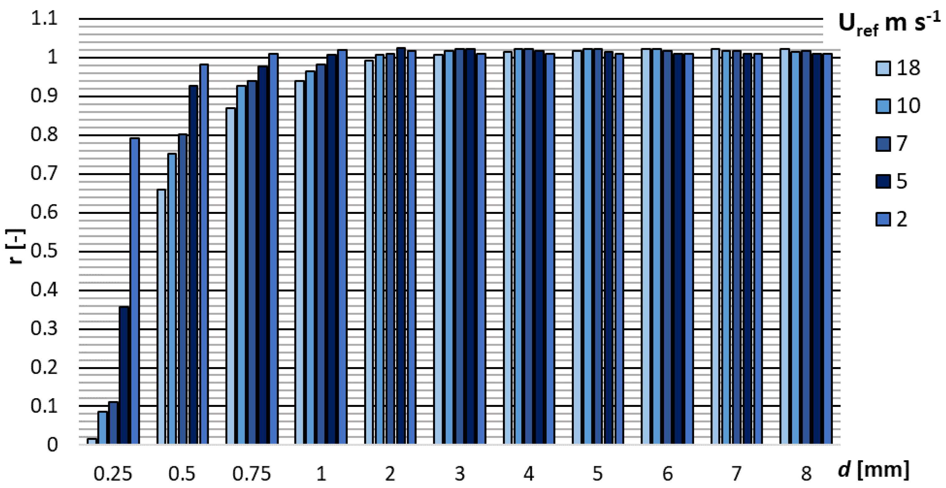
Starting from CFD simulations, the LPT model can obtain (per each particle size) the expected catch ratio,
r (-), defined as the ratio between the number of particles, which are captured by the gauge collector in disturbed airflow conditions,
n(
d), and the maximum number of particles,
nmax(
d), captured in undisturbed conditions. Catch ratios were computed for drops with equivalent diameter
d = 0.25, 0.5, and 0.75 mm and then from 1 to 8 mm, with bin size of 1 mm. These are compared in
Table 1 and
Figure 2 per each drop size and wind speed. For drop size less than 1 mm, the catch ratio increases with decreasing wind speed. For larger drops, the trend is not always growing, but increases and then decreases with increasing wind speed.
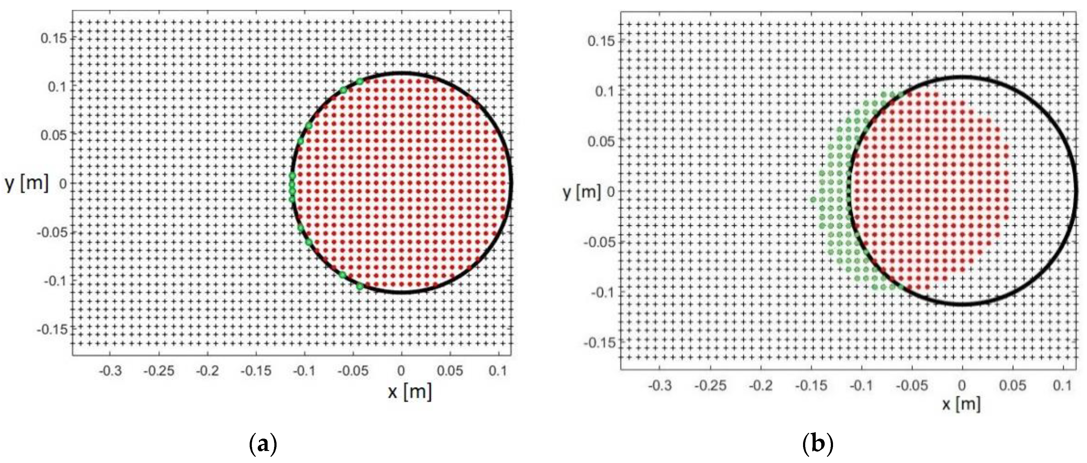
This behaviour is intrinsic in the balance between the drop size and the wind speed, and is graphically highlighted in
Figure 3. In the graph, a grid is reported where the releasing positions of the simulated drops are depicted with black markers. Drops are released in the simulated airflow field, upstream of the gauge, at a higher elevation than the collector area, depending on the wind speed and drop diameter. The proper location was preliminarily calculated to ensure that the released drops eventually fall in the region occupied by the gauge. This was obtained by computing backward the trajectory of a sample drop which reaches the centre of the gauge collector in undisturbed airflow conditions. The collector’s rim is depicted with black circles and contains the starting positions of those particles that, in undisturbed conditions, would enter the gauge collector.
The drop-releasing positions are colour-coded according to their destination. The initial positions of all drops that in real conditions are expected to fall inside the gauge collector and are actually collected are depicted in red, while those falling inside the gauge collector but were expected to fall outside are depicted in green.
The left-hand panel of
Figure 3 reports a low wind and/or heavy particle situation, and all drops that are expected to fall inside the collector in undisturbed conditions also reach the collector in the disturbed ones. A few additional drops, whose releasing positions are depicted in green, also enter the collector while being expected to fall outside. This implies an overestimation (
r > 1) of the precipitation collected by the gauge, and therefore the resulting catch ratio is larger than one. By increasing the wind speed, or reducing the drop size, the wind field deformation reduces the number of particles depicted with red dots, and slightly increases the green ones (right-hand panel of
Figure 3). In this sample case, the sum of the red and green dots is lower than the number of particles expected to fall inside the black circle, yielding an overall underestimation of the number of particles collected and
r < 1.
After introducing a suitable
PSD, indicating the number of particles
per unit volume of air and per unit size interval having a volume equal to the sphere of diameter
, the integral of the catch ratios over the range of diameters provides the numerical
CE in the form:
where
are the density and volume of particles with diameter
.
The
CE curve was derived from the calculated catch ratios by assuming that the microphysical characteristics of precipitation are those obtained from distrometer measurements in the Italian territory. The
PSDs, provided by [
27] for various
RI classes, were fitted with the typical exponential function [
28], hereinafter
MP), and the associated parameters
(intercept) and
Λ (slope) were adopted to calculate the
CE values (here called raw
CE values) per each
RI class.
A three-step procedure was used to derive a suitable parameterization of the CE curves based on rainfall intensity (RI), as follows.
First, in step (a), for each RI class, the CE curve was obtained as a function of wind speed () from the raw values of the numerical simulation results by fitting (with a least-squares method) a four-parameter sigmoidal function (CE = f()—see Equation (10)) and using the experimental and Λ parameters associated with each RI class.
The parameters and Λ used in step (a), attributed to the mean value of each RI class, were then fitted in step (b) with power law curves as a function of RI, and a new sigmoidal CE curve was obtained per each RI class from the fitted parameters. The definition of and Λ as a function of RI has the advantage of obtaining the MP parameters for any RI value, within the range investigated. After calculating the CE values for the associated RI and , the CE curves could be obtained again as a sigmoidal best-fit.
Finally, in step (c), to obtain a simple formulation for the CE as a function of both RI and in the investigated ranges, the four parameters of the sigmoidal function were also fitted with power laws or logarithmic curves as a function of RI.
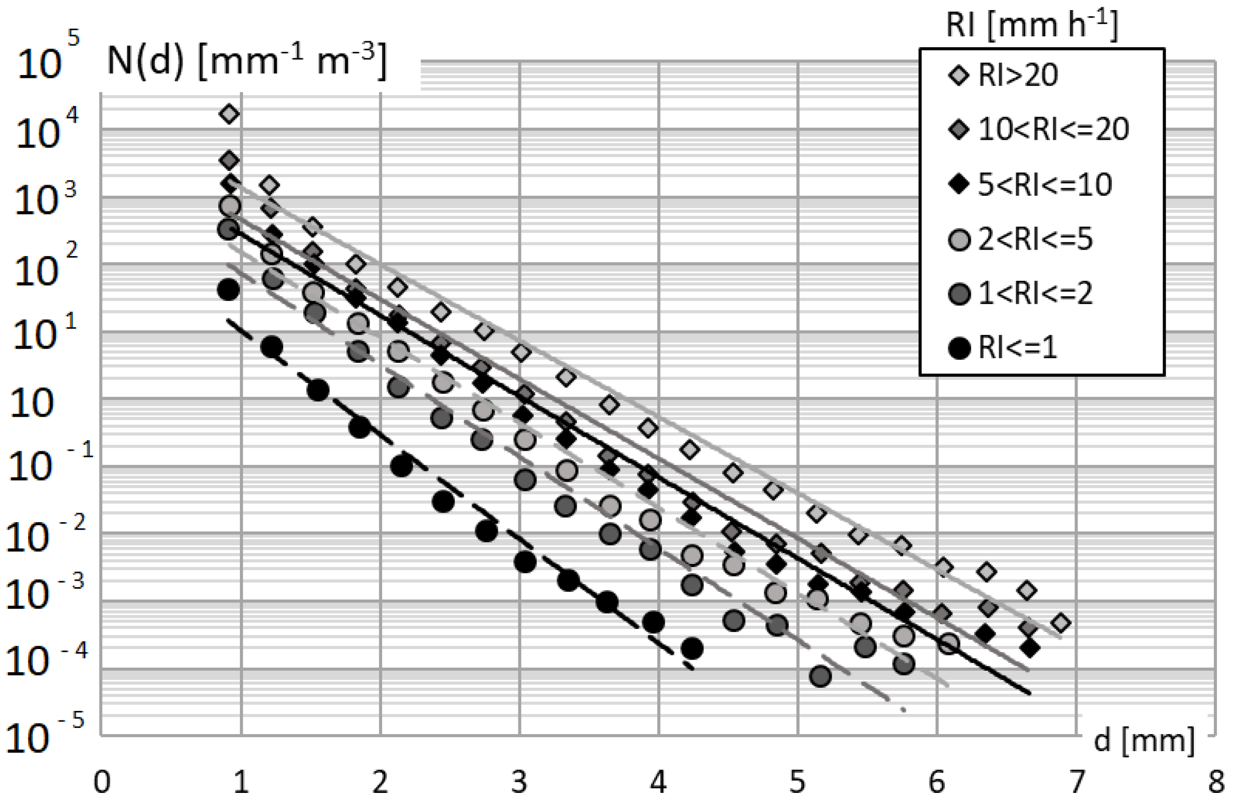
The procedure was applied to real-world observations. The average observed
PSD measured by the Pludix distrometer in the Florence experimental site, as provided by [
27], classified in six rainfall intensity classes, was adopted here and fitted using the typical
MP exponential function, as shown in
Figure 4. Some distrometers, including the Pludix, have limitations in detecting and counting small-size particles [
27]. Other instruments show a drop in the number of particles below 1 mm, although it is not clear whether this feature is inherent of the precipitation process or is a measurement bias. The exponential behaviour is here extended below 1 mm, down to a diameter of 0.25 mm. In general, small particles (lower than 0.25 mm) give a rather negligible contribution to the total volume of precipitation.
The
MP parameters
(mm
−1 m
−3) and
Λ (mm
−1), and the correlation factors (R
2) for each rainfall intensity class are listed in
Table 2.
As expected, the parameter Λ decreases with increasing RI, while increases. This is due to the fact that heavy rainfall events are characterized by a relatively higher number of drops of large diameter in the distribution and by an overall higher number of particles in one cubic meter of air. Therefore, by increasing RI, the slope of the distribution decreases and the curve is displaced upward. For all RI classes, the correlation factor is larger than 0.97, yielding a very good fit between the MP exponential curves and observations.
3. Results
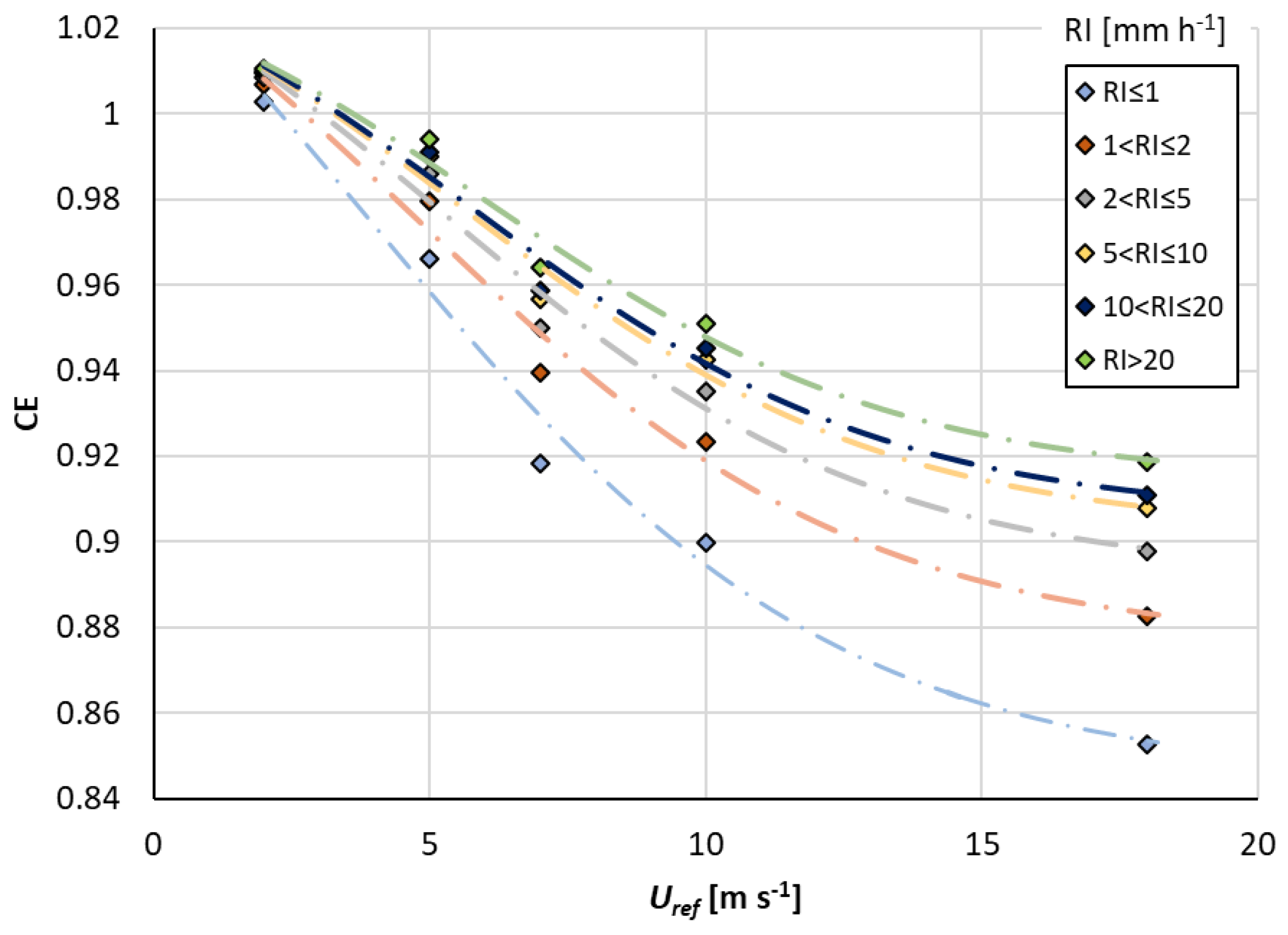
Following step (a), for each simulated wind speed (
), the raw
CE values were numerically calculated as reported in Equation (9), by using for the
PSD the best-fit
MP parameters associated with each
RI class (from
Table 2). Then, the obtained raw
CE values (diamonds in
Figure 5) were fitted with a four-parameter sigmoidal function (Equation (10) and dash-dot lines in
Figure 5). The obtained parameters’ values are listed in
Table 3 together with their associated R
2.
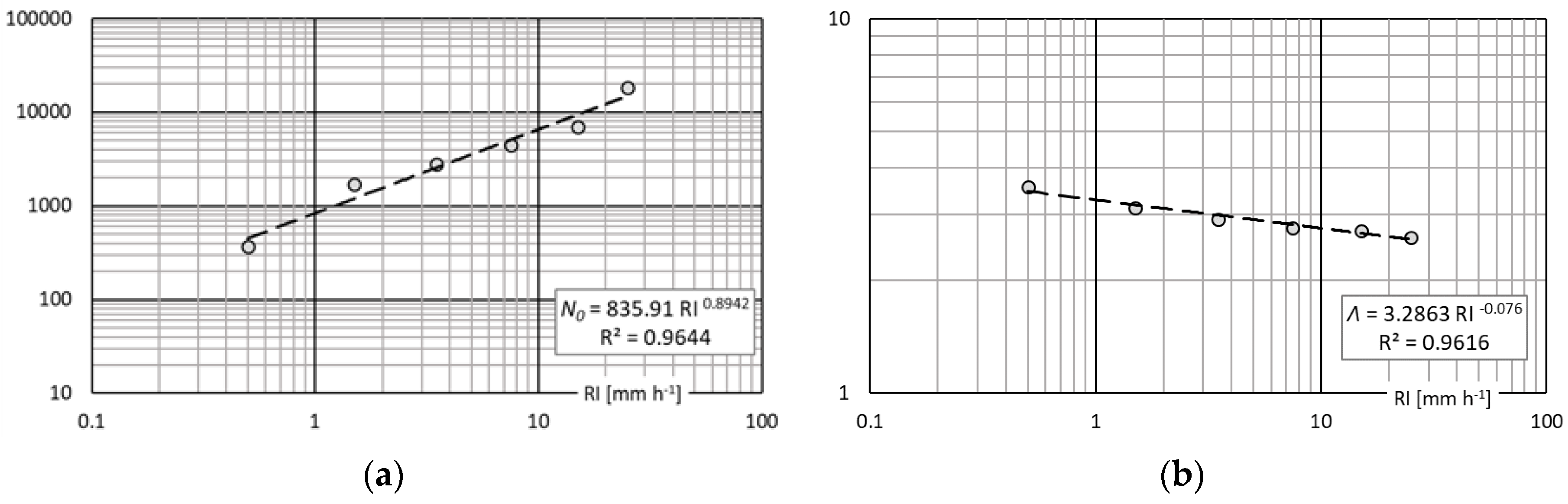
Following step (b), with the objective of making the dependence of the collection efficiency on the
RI explicit, the parameters
and
Λ were assigned to the mean value of each
RI class and fitted with power law interpolation curves (Equation (11)), as shown in
Figure 6.
In Equation (11),
assumes the nomenclature of the
PSD intercept
and slope
Λ, while
and
are the associated parameters of the best-fit power law curves. The values of the power law parameters are listed in
Table 4, together with the correlation factors for both
and
Λ.
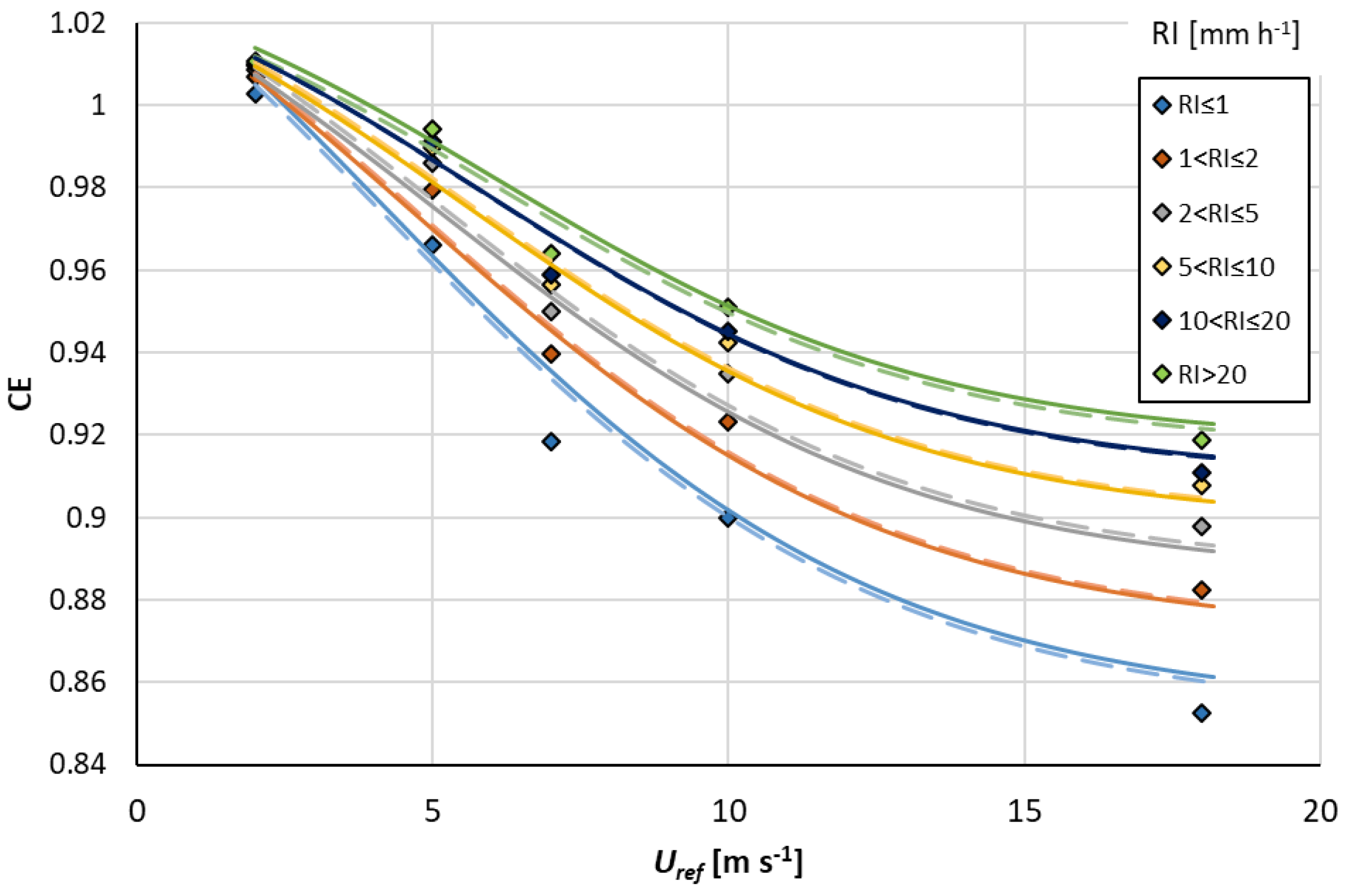
The
CE values were calculated by adopting the
and
Λ values provided by the power law curves (
Figure 6, dashed lines). The best-fit sigmoidal functions provide the new parameters for the
CE, as listed in
Table 5. The new
CE curves are depicted in
Figure 7 (dashed lines) and compared with the raw
CE values (diamonds) calculated under step a). This further step provides an important advantage because it allows to derive the
PSD for any desired rainfall intensity within the measured RI range (0.5–25 mm h
−1).
Finally, as summarized in step (c), a general formulation for the
CE Equation (12) as a function of both
RI and
, but independent of the initial
RI classes and valid throughout the investigated
RI range, was obtained by fitting the sigmoidal parameters associated with the mean value of each
RI class with logarithmic (for
,
,
) and power law (for the parameter
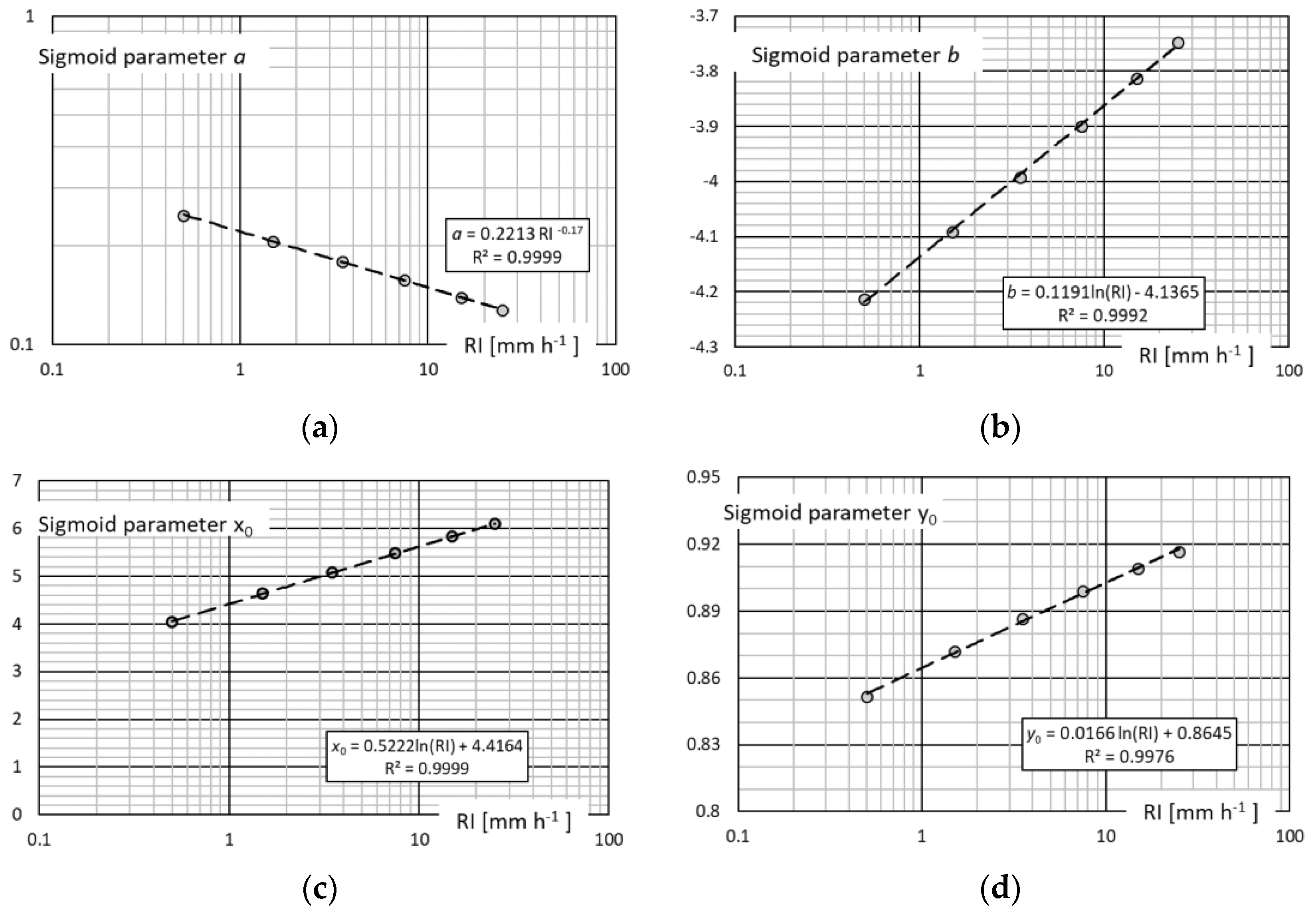
) curves.
The best-fit curves for each sigmoidal parameter
(a, , and
) as a function of
RI are listed below and shown in
Figure 8 with the associated correlation factors.
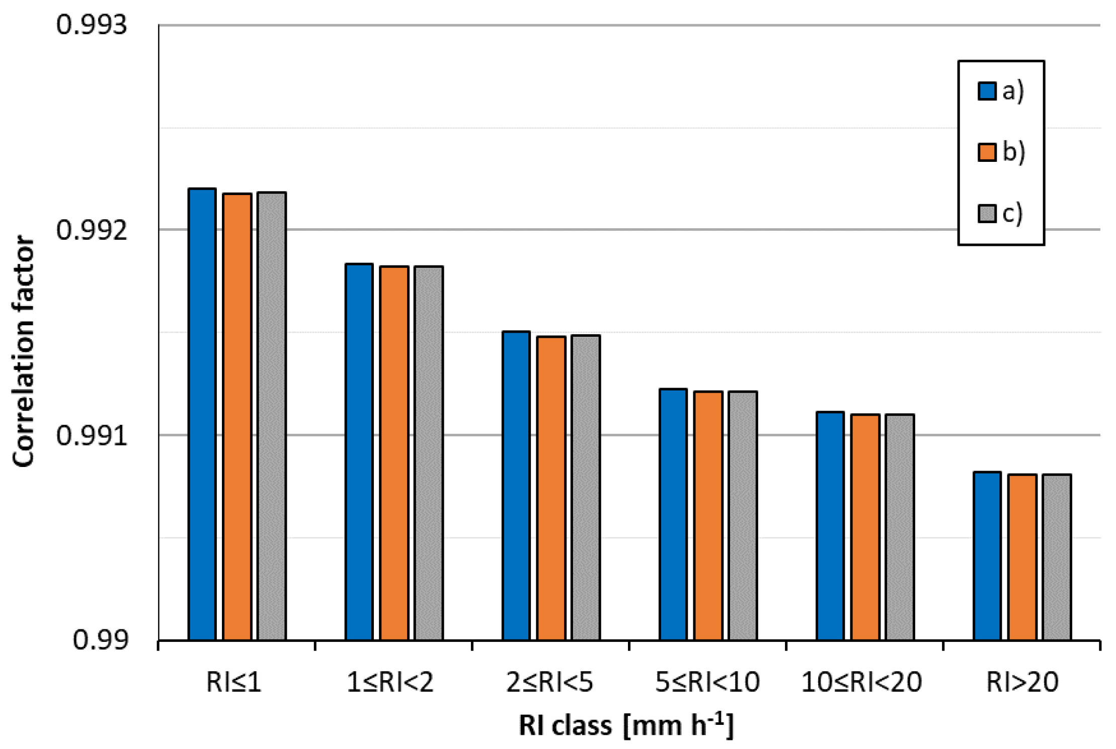
To verify the quality of this result, the collection efficiency curves were calculated by using Equation (12) for the mean value of each
RI class (
Figure 7, continuous lines), as already done in steps a) and b). Then, the correlation between the raw
CE values and the
CE curves obtained in the three steps (a–c) was compared.
Figure 9 shows the correlation factors for each
RI class and the partial step adopted ((a–c)). This result reveals that, in all cases, the correlation factors are very high, larger than 0.99, and only slightly higher for step (a) than for step (c) (about +10
−5). This very minimal worsening in performance is counterbalanced by the simplification introduced by the final
CE curve, which allows the easy application of a correction factor for the wind-induced bias of operational precipitation measurements.
The derived numerical
CE curve is a function of the actual rainfall intensity that, in this case, was obtained from the
PSD provided by [
27]. However, in operational practice, the only knowledge available for
RI is that measured by the gauge, which is therefore affected by the wind-induced bias. In this work, the adjustment curve was further derived, for application purposes, as a direct relationship between the reference rainfall intensity (
RI) and the measured one (
RImeas), so that the actual rainfall intensity (and the wind-induced bias) can be calculated starting from the measurement provided by the gauge, once the wind velocity is known.
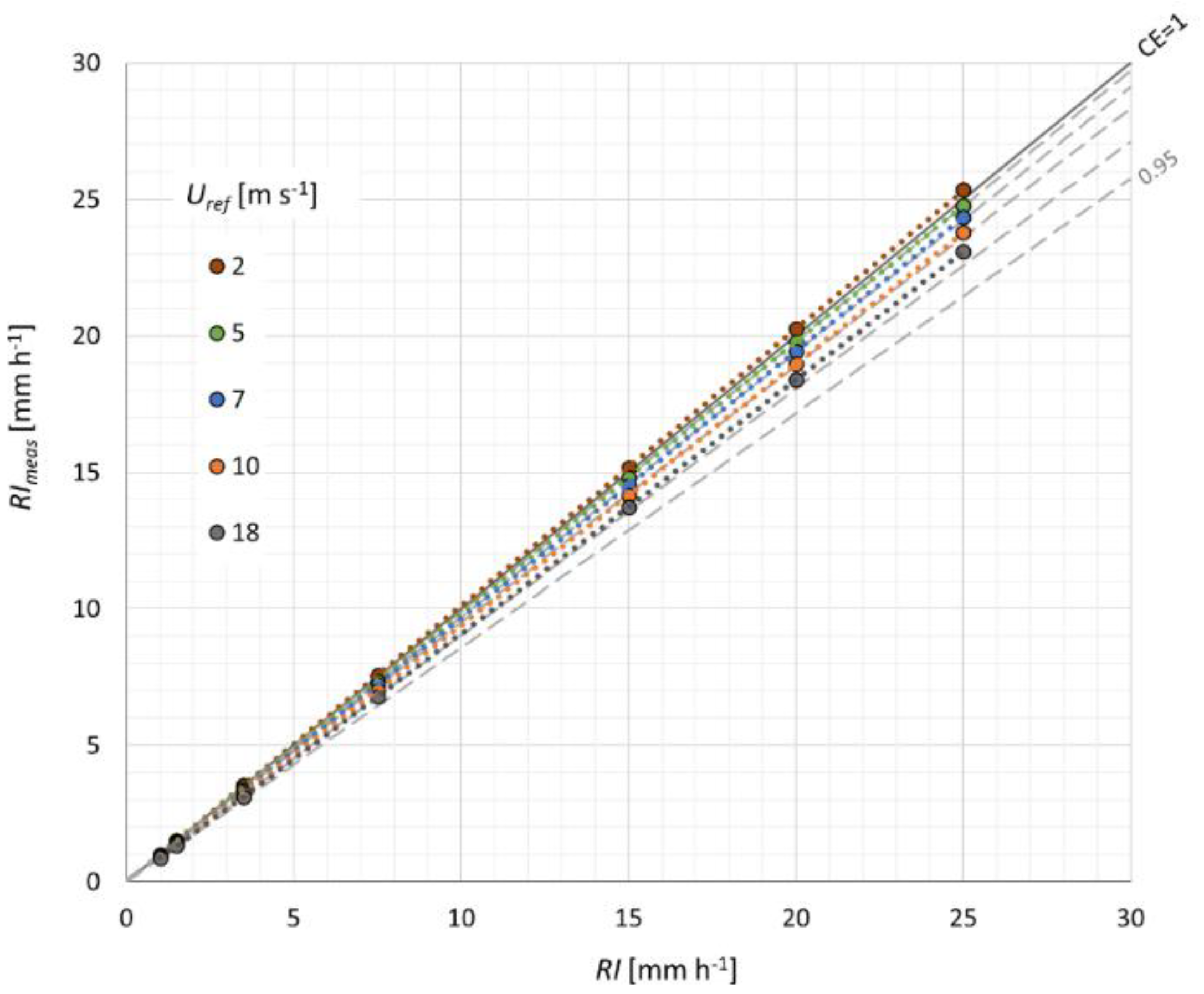
Recalling that, in the field, the
CE is defined as the ratio between the precipitation measured by the gauge (
RImeas) and the reference one (
RI), it is possible to derive from Equation (12), the
RImeas associated with each (
,
RI) couple within the investigated range. The results can be depicted in the (
RI,
RImeas) plane for each wind speed, as shown in
Figure 10. The
RImeas values calculated from Equation (12) for the mean values of each
RI class and the simulated wind speed are depicted with markers, while the associated adjustment curves were obtained as best-fit power law curves as follows:
The coefficient α and exponent
β of the adjustment curves for the simulated wind speed are summarized in
Table 6, with a correlation factor (
R2) equal to one (1.000) in all cases, and their functional dependency on wind speed is expressed in Equations (18) and (19). The correlation factor is equal to 0.973 and 0.997 for
α and
β, respectively.
In
Figure 10, the diagonal (continuous black line) indicates
CE = 1, while the grey dashed lines correspond to
CE values from 0.95 to 0.99. As expected, the adjustment curve for
= 2 m s
−1 is located above the diagonal, due to the overcatch observed at this low wind speed, while the other curves are lower due to the wind-induced undercatch. Moreover, the adjustment curves are described by power law functions, with coefficients (see
Table 6) that are increasingly different from one (the linear case when
CE is constant) as the wind speed increases, reflecting the trend towards higher values of
CE while the rainfall intensity increases.
Although the deviation is small, it is possible to note in the graph that the adjustment curve at e.g., 18 m s
−1 progressively diverges from the dashed line at
CE = 0.96 with increasing rainfall intensity (towards the right-hand side of the graph), while they are practically superimposed to each other at a low
RI (left-hand side of the graph). This means that, at any given wind speed, the collection efficiency varies with the rainfall intensity, rather than lying on a curve (line) at
CE = constant, as predicted by the existing experimental studies (e.g., [
14]).
4. Discussion
Adjustment curves for a typical, cylindrical gauge as a function of wind speed were derived from numerical simulation, including a new parameterization based on the measured rainfall intensity. A simple formulation of the adjustment curves was obtained, which can be easily applied in an operational context. Wind velocity is the only ancillary variable required to perform the adjustment and, since wind is often measured by operational weather stations together with the precipitation intensity, its use adds no relevant burden to the cost of meteo-hydrological networks.
The functional dependency of the
CE curves on rainfall intensity is demonstrated in this work for a cylindrical, catching-type gauge and the results confirm that such a parameterization holds for liquid precipitation measurements, as was demonstrated already by [
14] for snowfall measurements, using a chimney-shaped weighing gauge. Using
RI as a controlling factor for the
CE has sound physical bases in the relationship between
RI and the
PSD, and the role of
RI can only be quantified using numerical simulations of both the airflow field (CFD) and the particle motion (LPT). Reference [
14] also demonstrated that the application of this rationale to field test data helps in reducing the scatter of the observations. Further developments of the present work would include extensive validation with suitable experimental campaigns where contemporary
RI and wind velocity data are available, together with a reference rain gauge pit. The role of free-stream turbulence in attenuating the updraft and acceleration of the airflow above the collector as shown in [
29], and its effect on the adjustment curves could also be quantified.
Application of the results presented in this work spans over many fields of hydrology, meteorology, and climatology, including water resources and flood risk management and agriculture. Rainfall is indeed the forcing input of the land phase of the hydrological cycle. The knowledge of rainfall, its variability and the observed/expected patterns of rain events in space and time, are of paramount importance for most hydrological studies, and a large number of consequences of such studies on the engineering practice are exploited in the everyday technical operation. The results, especially the proposed adjustment curves, have the potential to improve rainfall measurements in order to support the enhanced accuracy and reliability of the basic information used in many engineering applications such as the design of hydraulic works, the protection from flood-related hazards, the management of potable water supply and its conservation, hydropower production, the enhancement of sustainability and resilience of human settlements and the conservation and protection of the natural and cultural heritage.


