1. Introduction
Sewer networks are a critical piece of infrastructure that allow safe transportation of wastewater from households to specialized treatment plants. Sewer pipes are built for transporting either rain water, waste water, or a combination of both. In Germany, there are nearly 600,000 kilometers of public sewer pipes [
1]. In the US, it has been estimated that the length of public net of sewers extends to over 1.2 million kilometers [
2]. Because the sewer pipes are buried beneath roads and streets, their presence is easy to forget—until they break down. Replacement of an entire sewer pipe is costly and can require a large excavation work that entails disruptions to the road traffic. A more economical option is to refurbish the pipes before they break down [
3], but this requires knowledge of the condition of the pipes. However, sewer pipes are difficult to inspect as most pipes are not accessible by human inspectors due to their small diameters. For large diameter pipes, the presence of toxic gases and the general contents of the sewage water renders the inspection a safety and health risk to human workers. The most common method for estimating the condition of a sewer pipe is to use tethered robots that are inserted into the pipe from the nearest accessible well. The inspection robot is typically equipped with a Closed-Circuit Television camera (CCTV) and a light source. A human operator controls the robot from a specially designed van and manually assesses the incoming video data. The overall inspection procedure is slow and prone to human errors. Therefore, there is a large research and industrial interest in automating the inspection process through the use of computer vision and machine learning [
4].
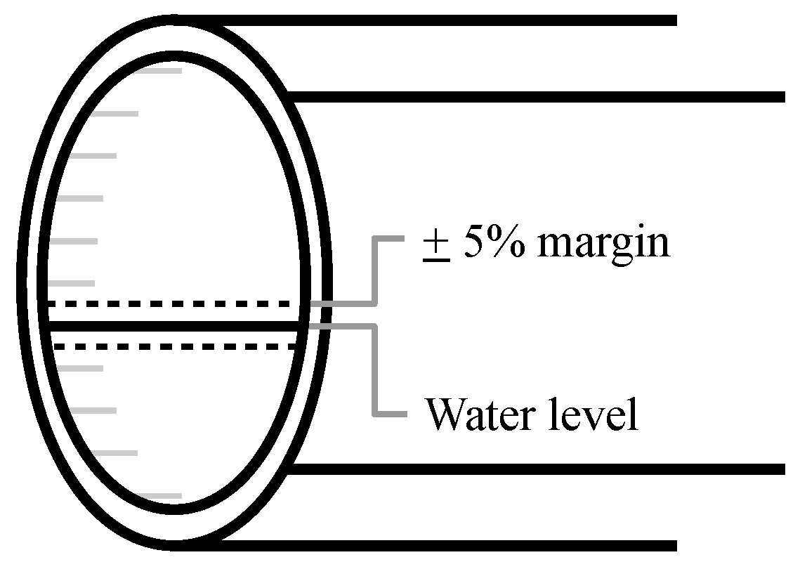
Accessibility of the sewer for inspection by a robotic platform is one of the most fundamental problems the inspection has to address. The accessibility is linked to the amount of water present in the pipe. In order to detect and classify defects in the pipe, substantial portions of the pipe must be visible above the water level. In short, the water level is a key indicator of how much of a pipe can be inspected. According to the European sewer inspection standards (EN 13508-2) [
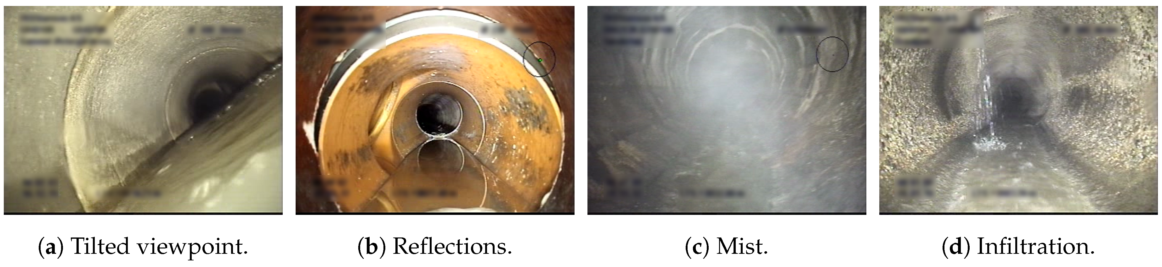
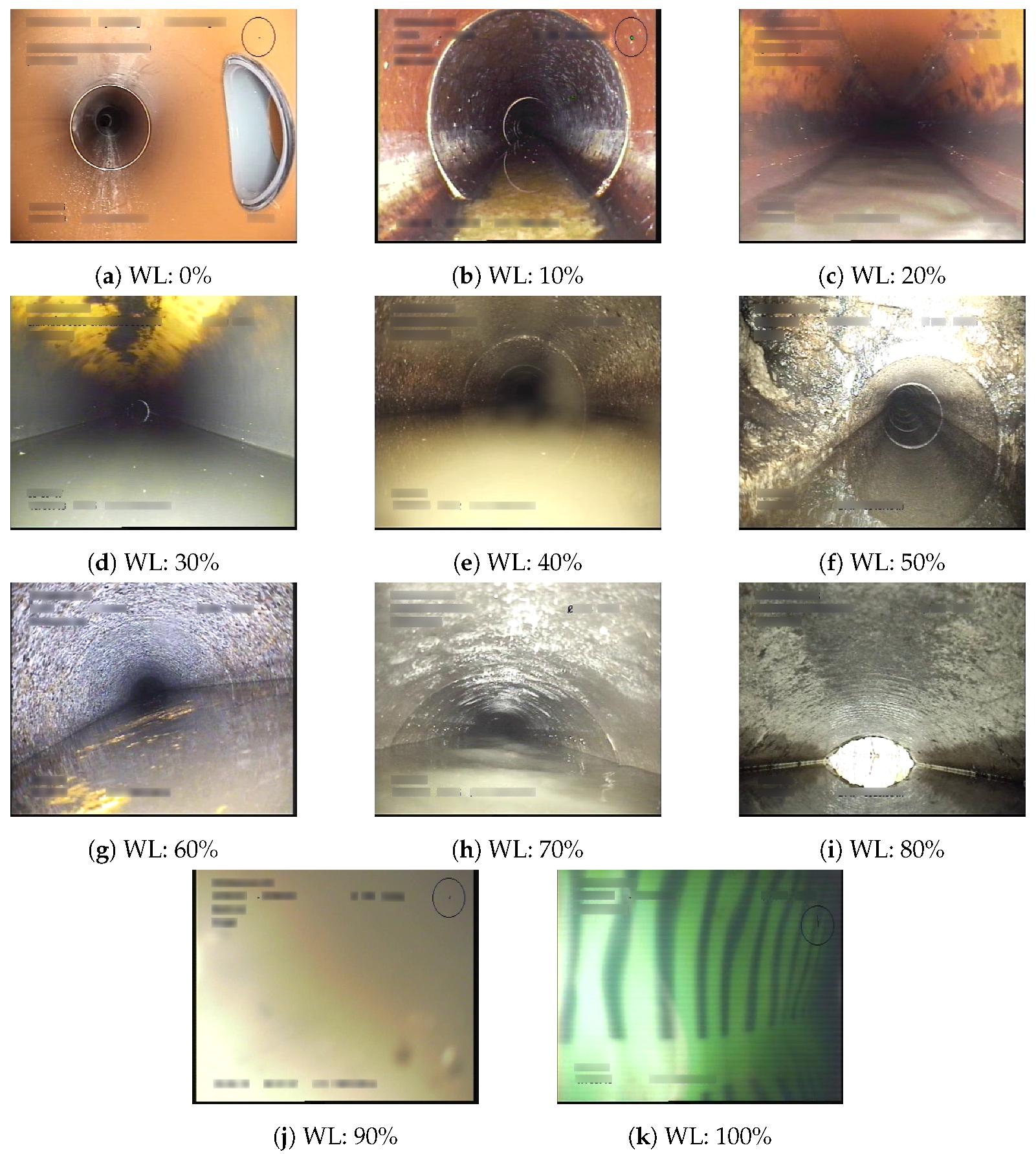
5], estimating the water level of the sewer pipe is therefore of paramount importance to human inspectors. Sample footage from inspection data is shown in
Figure 1. At first sight, estimating the water level from sewer pipes might appear to be a straightforward task for a computer vision algorithm to solve. The sewer is a confined space with few interruptions from the outside. However, the nature of the pipes and their contents renders a range of problems. The only source of light comes from the inspection vehicle, and some portions of the pipe might therefore not be sufficiently lit. Toxic gases are commonplace and renders as mist or fumes, resulting in a hazy image with reduced information. The presence of water entails different levels of reflection and might even flood the entire view. As a result, dust and sewage might stick to the lens and severely impair the visibility.
While there has been a lot of prior work on sewer defect classification and detection, as surveyed by Haurum and Moeslund [
4], few researchers have worked specifically with water level estimation. Prior work utilizes classical computer vision techniques and modern deep learning-based methods. Classic computer vision methods have been used to detect key features of the sewer pipe which can be used to detect the water line [
6,
7]. Recently, Convolutional Neural Network (CNN)-based methods have gained interest in automated defect classification [
7,
8,
9], wherein some researchers have included water stagnation [
8] and “high water levels” [
9]. Most importantly, a recent paper [
10] proposed training a deep learning-based segmentation model which segments the water in the image and infers the water lines. The researchers collected 1440 high-resolution RGB images, of which 167 were used for human evaluation and 80 images were used for training. The authors claim to achieve a perfect segmentation of the water level, beating manual and traditional computer vision annotation methods, and being able to calculate the flow rates and velocities by applying Manning’s equation. However, their dataset only consists of recordings from a single pipe acquired over a 24-h period. This does not nearly capture the amount of variability encountered when inspecting real sewers. Furthermore, the high image resolution is not representative for sewer inspection CCTV videos which rarely exceeds full HD.
Several vision-based approaches for water level estimation have been proposed within the wastewater flow estimation field. A common technique is to measure the depth from a stationary staff gauge [
11,
12,
13,
14,
15]. Nguyen et al. [
11] and Jeanbourqin et al. [
12] proposed to use an infrared camera to locate the water–air intersection line on the staff gauge using computer vision techniques. Handheld devices [
15] and calibrated cameras [
13,
14] have also been used for automated staff gauge readings. Alternatively, Sirazitdinova et al. [
16] determined the water level using a stereo camera setup, while Khorchani and Blanpain [
17] used a single calibrated camera. A common characteristic among these methods is the need for a stationary object, being either the camera setup or the staff gauge.
On the contrary, we investigate the feasibility of estimating the water levels in realistic and unseen sewer inspection videos by the use of a single input image at a time, from a moving uncalibrated camera. We compare both decision tree methods and deep learning-based methods in order to determine whether the extra complexity introduced with the neural networks is justified. Furthermore, as shown from the examples of
Figure 1, the inspection imagery is distinct from commonplace computer vision datasets such as ImageNet [
18] or COCO [
19]. Therefore, we investigate the effect of ImageNet pre-training compared to training from scratch on the available data. Our contributions are the following.
We show that it is possible to reliably estimate the water level in unseen sewer pipes using a classification-based CNN.
We show the evaluation performance impact of how the water levels are categorized, using the Danish sewer inspection standards as a use case.
We show that CNN-based methods outperform traditional decision tree-based methods for water level estimation.
The remainder of the article is structured as follows. In
Section 2, we introduce our dataset. In
Section 3, we describe the proposed methods, loss functions, and the training procedure. In
Section 4, we detail the evaluation metrics and present the experimental results. In
Section 5, we analyze and discuss the presented results. Finally, in
Section 6 we summarize our findings and possible future directions.
3. Methodology
We investigate the performance of multiple machine learning methods using both the 2010 and 2015 Danish annotation guidelines. First, we train the proposed models using the annotations following the 2010 standard in a classification approach where each level is a discrete class. Second, we train the models in a regression setting where the water level percentage is predicted as a continuous quantity. Last, we train the models in a classification setting and convert the annotations to the 2015 standard classes where the different classes are grouped as mentioned in
Section 2. These settings are referred to as Class10, Reg2Class10, and Class15, respectively.
3.1. Features and Models
We investigate the performance of two CNNs—AlexNet and ResNet—to determine whether deep learning is feasible for estimating the water level in sewers from single images. Furthermore, by measuring the performance of ResNet-18, ResNet-34, and ResNet-50, we can evaluate the effect of higher abstraction levels provided by an increased network depth.
AlexNet [
22] is considered to be the deep neural network that sparked the interest for deep learning almost ten years ago, and it is often used as a baseline for classification tasks. A neural network is considered deep when there is more than a single layer between the input and output layers, and AlexNet has eight such layers. Generally speaking, the feature abstraction level increases with the depth of the network which, in theory, means that a deeper network can handle more complex tasks. However, as the amount of parameters increases, so does the processing time and the likelihood of overfitting the model to the training data. It has even been shown that for some architectures it can harm the performance if the depth is overly increased due to the degradation problem [
23].
ResNet [
24] is a family of CNN models developed with the aim of being able to utilize the increased abstraction level offered by deeper layers without suffering from the degradation problem. The models consist of stacks of relatively small layers connected by identity shortcuts that forces the network to learn the residual function between the stacks. These shortcuts allow the networks to cheaply reduce the influence of certain layers if they do not enhance the output performance. This type of architecture has proven to be very powerful and ResNets are still widely used; especially for cases where depth is expected to improve the performance.
Two decision tree methods—Random Forest [
25] and Extra Trees [
26]—are also investigated in order to provide a baseline performance. The tree-based methods are trained using GIST features [
27] computed from the images as Myrans et al. The authors of [
28] have shown this to be an effective combination for sewer defect classification. The GIST feature descriptor [
27] applies a series of 2D Gabor filters, each with a different scale and orientation, resulting in a feature map per scale and orientation permutation. The feature maps are divided into a predefined grid where the feature values within each grid element are averaged. The averaged feature values are then concatenated per feature map into a feature vector, and all of the resulting feature vectors are concatenated to give the final GIST feature vector.
3.2. Loss Functions
The classification models are all evaluated using the standard categorical cross-entropy (CE) loss with the option of including class specific weights,
. The cross entropy loss is defined as
where
is the ground truth label, 1 if the correct class, and 0 otherwise, and
is the predicted probability of class
c. For the standard CE loss,
is set to 1 for all classes.
However, for the regression networks there is not a single standard loss. A large set of methods utilizes the Mean Absolute Error (MAE) or Mean Square Error (MSE) loss functions, also known as the
and
loss functions, respectively. MAE and MSE are defined as
where
x is the residual, the result after subtracting the predicted value from the ground truth value.
The MAE loss function is robust to outliers but suffers from derivatives that are not continuous. MSE is more stable during training due to continuous derivatives, but more sensitive to outliers due to the squared residual term. Due to the built-in uncertainty around each annotation in the 2010 standards, we choose to train with the MSE loss as the quadratic residual term allows automatically increasing the weighing the further away the prediction is from the ground truth.
3.3. Training Procedure
The CNNs are all trained using the hyperparameters stated in
Table 3. The Adam optimizer [
29] is chosen as it continuously adapts the learning rate for each parameter based on the first- and second-order moments of the gradients. The initial learning rate is set to
for models learned from scratch whereas a reduced learning rate of
is used for fine-tuning networks pretrained on the ImageNet dataset. When fine-tuning the ResNet models, we freeze the first two residual blocks in order to retain low-level feature knowledge. A weight decay of
is used for all models to help regularize the weight parameters and avoid overfitting. All models are trained for 50 epochs with a batch size of 64 to make them comparable. During training, the input images are augmented by horizontally flipping the image with a 50% chance. All images during both training and evaluation are normalized.
We conduct a small hyperparameter search in order to find the best set of parameters for the tree-based methods. The investigated hyperparameters and the possible values are shown in
Table 4, where
d is the amount of features in the GIST feature descriptor. For the classification models, the minimum number of samples required to be at a leaf node is set to 1, whereas for the regression models it is set to 5, as per the original Random Forest paper [
25]. The GIST feature descriptor is computed using a
grid with filters using 4 scales and 8 orientations. The input image is downscaled to
pixels and converted to grayscale as described in [
28], which results in a 512 dimensional GIST feature vector.
All classification models are trained by minimizing a weighted CE loss where the class weights are calculated as
where
is the number of training samples for class
i and
is the weight for class
c, out of the total
C classes.
The regression models are trained by minimizing the MSE loss. The best performing model is determined by selecting the model with the lowest validation loss. For the CNNs, the validation loss is computed after each epoch. The best performing tree-based models are found from the model with the lowest validation loss among the models in the aforementioned hyperparameter search, see
Table 5.
All of the CNN architectures are implemented using the PyTorch framework [
30], utilizing the publicly available implementations as well as the provided network weights for the ImageNet pretrained models. The models were trained on a single RTX 2080 TI graphics card. For the tree-based models, we utilize the Scikit-Learn library [
31] while the GIST features are extracted using an open source Python wrapping of the original C implementation [
32].
5. Discussion
From the results presented in
Table 6 it is possible to see several trends. We observe that utilizing the 2015 classification scheme leads to a direct increase in performance compared to the 2010 standard. Specifically, we see that for all models, except AlexNet-FT, the F1-metrics have been improved dramatically. This corresponds with prior research by Van der Steen et al. [
33], who found that the more detailed a sewer inspection standard is, the more mistakes inspectors make.
When looking into the training settings, we see that the classification approaches consequently match or outperform the methods trained with a regression approach. This indicates that the strict discrete class membership enforced by the classification approaches leads to better generalization than the soft continuous class membership enforced by the regression approaches. This may be a direct consequence of all the ground truth labels being discrete values with a known uncertainty margin, leading to the values actually representing a span of values. The regression approaches may, however, perform better if the ground truth labels were provided by a continuous measurement such as data from a flow meter.
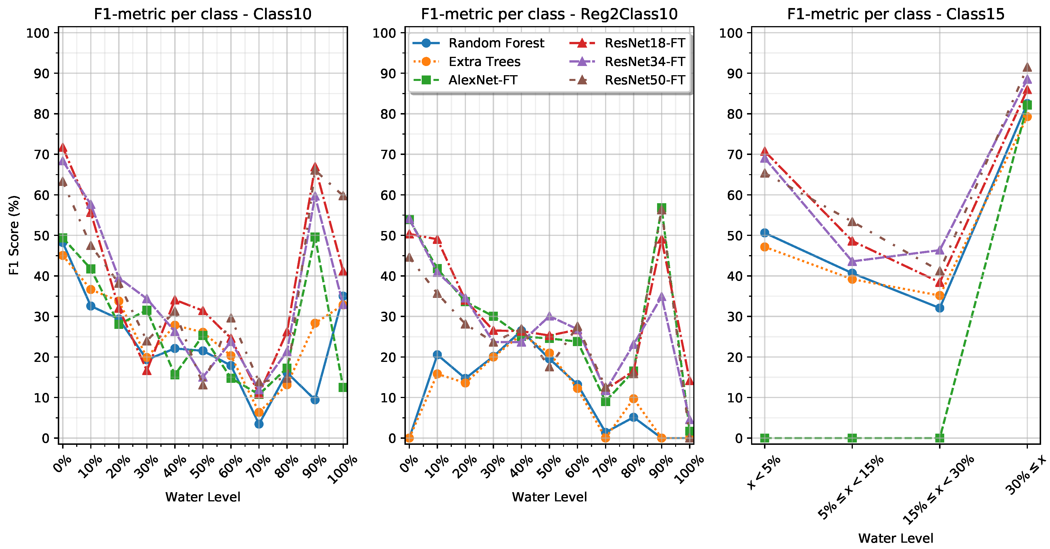
When looking into the class-specific performance of the Class10 and Reg2Class10 training settings in
Table 8 and
Table 9, we observe that the models have a high F1-metric for the first few classes where the water level is still visually distinguishable. However, as the water level increases, the F1 metric performance decreases until an increase in performance for the 90% and 100% water level classes. We see that for the tree-based methods in the Reg2Class10 setting, there are several classes with an F1-metric of 0% while other classes have an F1 metric of up to 26%. Similarly, we observe that the AlexNet-S model simply focuses on a single class in its predictions as also shown by the Macro-F1 score, while the AlexNet-FT model is capable of producing more meaningful predictions. We also see that the depth of the networks does not seem to correspond with an increase in performance of the F1-metric.
It is observed that the tree-based methods do not match the micro-F1 score of the ResNets and AlexNet for the Class15 training setting. However, when comparing the Macro-F1 metric, it is obvious that the tree-based methods outperform the AlexNet on some classes. By looking into the results in
Table 9 we see that the tree-based models perform well on the two extreme classes, <5% and ≥30%, but are not as capable at classifying the two intermediate classes where the inter-class variance may be more subtle. Moreover, we see that the AlexNets do not generalize at all, instead simply collapsing to predict only the majority class. This is in contrast with how the AlexNets performed in the Class10 and Reg2Class10 training settings, where only AlexNet-S failed to produce meaningful predictions.
These results show that by framing the water level estimation task as a clustering of perceptible amount of water, as in the 2015 Danish standards, better facilitates machine learning-based methods than using a direct mapping such as in the 2010 Danish standards. However, the results are not perfect, as there are still some classes with a low classification rate. This could potential be improved by including temporal information in the models, such that transitions between water levels can be detected and spurious classification be ignored. Such an approach has been applied by the authors of [
28], who applied a Hidden Markov Model and window filtering to sewer defect classifications. Geometric information, such as the size and shape of the pipe, may also prove useful as these are closely linked with the water level. Last, information about defects would also help guide the models toward the correct water level classification. Defects such as pipe collapse or large roots could lead to abnormally high water levels.
6. Conclusions
Estimating the water level in sewers during inspection is important as it indicates the portion of the pipe that cannot be visually inspected. Currently, it is a subjective and difficult task of the inspector to estimate the water level through CCTV recordings and only limited research has been conducted on automating this process. A professionally annotated dataset with 11,558 CCTV sewer images provided by three Danish utility companies is used as the foundation for an investigation on the feasibility of using deep neural networks for automating water level estimation. The problem is studied through two classification tasks following the 2010 and 2015 Danish Sewer Inspection Standards. Four deep neural network models (AlexNet, ResNet-18, ResNet-34, and ResNet-50) and two traditional decision tree methods (Random Forest and Extra Trees) are compared against each other.
The deep learning methods generally outperform the decision trees, but the networks do not seem to benefit from the abstraction levels of the very deep layers. The best results are provided by ResNet with micro-F1 scores of 39.70% and 79.29% following the 2010 and 2015 standards, respectively. These are promising results given that the data are noisy and the classifications are based on single images. Utilizing temporal, contextual, and geometric information could improve the classification rate and should be considered for future work.


