Article

Impact of Nutrients, Temperatures, and a Heat Wave on Zooplankton Community Structure: An Experimental Approach

1
Limnology Laboratory, Department of Biology, Middle East Technical University, Ankara 06800, Turkey
2
Ecosystem Research and Implementation Center, Middle East Technical University, Ankara 06800, Turkey
3
Centre for Water Technology (WATEC), Department of Bioscience, Aarhus University, 8600 Silkeborg, Denmark
4
Key Laboratory of Aquatic Botany and Watershed Ecology, Wuhan Botanical Garden, Chinese Academy of Sciences, Wuhan 430074, China
5
Institute of Agricultural and Environmental Sciences, Estonian University of Life Sciences, 51006 Tartu, Estonia
6
Sino-Danish Centre for Education and Research, University of Chinese Academy of Sciences, Beijing 100380, China
7
Environmental Health Program, Eldivan Vocational School of Health Services, Çankırı Karatekin University, Çankırı 18700, Turkey
8
Institute of Marine Sciences, Middle East Technical University, Mersin 33731, Turkey
*
Authors to whom correspondence should be addressed.
Water 2020, 12(12), 3416; https://doi.org/10.3390/w12123416
Submission received: 16 October 2020 / Revised: 30 November 2020 / Accepted: 1 December 2020 / Published: 4 December 2020
(This article belongs to the Special Issue Effect of Extreme Climate Events on Lake Ecosystems)

Abstract

:
Shallow lakes are globally the most numerous water bodies and are sensitive to external perturbations, including eutrophication and climate change, which threaten their functioning. Extreme events, such as heat waves (HWs), are expected to become more frequent with global warming. To elucidate the effects of nutrients, warming, and HWs on zooplankton community structure, we conducted an experiment in 24 flow-through mesocosms (1.9 m in diameter, 1.0 m deep) imitating shallow lakes. The mesocosms have two nutrient levels (high (HN) and low (LN)) crossed with three temperature scenarios based on the Intergovernmental Panel on Climate Change (IPCC) projections of likely warming scenarios (unheated, A2, and A2 + 50%). The mesocosms had been running continuously with these treatments for 11 years prior to the HW simulation, which consisted of an additional 5 °C increase in temperature applied from 1 July to 1 August 2014. The results showed that nutrient effects on the zooplankton community composition and abundance were greater than temperature effects for the period before, during, and after the HW. Before the HW, taxon richness was higher, and functional group diversity and evenness were lower in HN than in LN. We also found a lower biomass of large Cladocera and a lower zooplankton: phytoplankton ratio, indicating higher fish predation in HN than in LN. Concerning the temperature treatment, we found some indication of higher fish predation with warming in LN, but no clear effects in HN. There was a positive nutrient and warming interaction for the biomass of total zooplankton, large and small Copepoda, and the zooplankton: phytoplankton ratio during the HW, which was attributed to recorded HW-induced fish kill. The pattern after the HW largely followed the HW response. Our results suggest a strong nutrient effect on zooplankton, while the effect of temperature treatment and the 5 °C HW was comparatively modest, and the changes likely largely reflected changes in predation.

1. Introduction

Lakes, the overwhelming majority of which are shallow, cover only 3% of the world’s surface [1,2] but are biodiversity hotspots that provide significant ecosystem goods and services [3,4]. Today, shallow lakes are severely threatened by eutrophication, climate change, and their combined effects [5,6]. Global warming not only increases the average temperature but also enhances the frequency, intensity, and duration of extreme events such as heat waves [7,8,9,10]. Although no universal definition of “heat wave” (HW) exists [8], periods of abnormally hot weather affect the structure and function of freshwater systems. The frequency of HW is increasing [10], and HWs may affect both the physico-chemical conditions [11] and biota in lakes, as well as their interactions [12,13,14].
Zooplankton play an important role in the food web of shallow lakes, being placed at the intermediate trophic level linking fish and phytoplankton, and they contribute to maintaining clear water conditions and respond to eutrophication [15,16,17]. They are also sensitive to increasing temperatures, directly affecting their ontogeny and physiology and indirectly altering their sources of food [18,19,20]. Furthermore, several comparative studies have reported that increasing temperatures shape zooplankton communities through changes in fish communities, affecting the predation pressure on zooplankton (e.g., [21,22,23]). In heated mesocosms without fish, Strecker et al. [24] found a decrease in zooplankton biomass, especially that of large-sized cladocerans, and they suggested it to reflect a taxonomic shift in the composition of phytoplankton towards larger sizes, including toxic and less edible cyanobacteria, as seen in several studies [25]. A pan-European mesocosm experiment also showed a decrease in large-sized zooplankton along an increasing temperature gradient [26]. Temperature itself may also affect body size. The metabolic theory of ecology (MTE) suggests that body size decreases with increasing temperature [27], and declining body size is proposed to be a universal response to warming [28,29,30,31]. A study covering lakes at a latitude from 6° to 74° recorded a reduction in Cladocera body size with increasing temperatures [32], but in this and other studies [5,23] it was attributed to a parallel-occurring increase in fish predation.
Whether nutrient or temperature is of key importance in shaping the zooplankton community is debatable, but a recent cross-system analysis from mesocosms and lakes found an overall stronger effect of nutrients than of temperature on various biota in lakes and streams [33].
Several previous studies have revealed significant adverse effects of warming on freshwater ecosystems (e.g., [34,35,36,37]), but there are only a few studies with a focus on the impact of HW on lakes, particularly on the zooplankton. In this study, we explored the response of zooplankton community composition, biomass, diversity, and size structure to differences in nutrient concentration, temperature, and to a one-month artificial HW in mesocosms run at different temperatures according to the Intergovernmental Panel on Climate Change (IPCC) warming scenarios (A2 and A2 + 50%) crossed with low and high nutrient loading. The mesocosms used in our study are part of the longest running (since 2003) warming lake experimental facility in the world [38,39]. We hypothesized that: (1) eutrophication would have an overall stronger effect on the zooplankton community structure and functioning than relevant increases in temperature/HW due to global warming, (2) eutrophication would potentially increase the zooplankton biomass due to higher food availability unless planktivorous fish predation in the absence of piscivorous fish would prevent it. (3) Enhanced temperature and the HW would result in reduced zooplankton biomass, not least the large-bodied specimens, due to increased fish predation at the higher temperatures, unless the HW led to fish kill or fish spawning were affected negatively by higher temperature, as seen in some studies [34], and (4) the size diversity of the zooplankton community would be significantly reduced by an increase in nutrients and temperature/HW at both low and high nutrient concentrations due to selective predation on large-bodied specimens.

2. Materials and Methods

2.1. Experimental Setup

A mesocosm experimental facility in Lemming (Central Jutland, Denmark; 56°14′ N, 9°31′ E), which has been running since 2003, was used for our study. The setup contains 24 outdoor cylindrical stainless-steel tanks with a diameter of 1.9 m and a depth of 1.5 m in which the water is fully mixed by paddles. The sediment consists of a mixed 0.1 m layer of washed sand and a 0.1 m layer of nutrient-rich sediment (mainly coming from a nearby natural freshwater pond) that has been passed through a net (mesh size: 1–2 cm) to avoid uncontrolled vegetation and vertebrates. It is a flow-through system receiving tap water 6 times per day and has a water residence time of approximately 2.5 months.
The experimental design included a combination of three temperature scenarios and two different nutrient levels (four replicates): unheated (ambient, hereinafter A0) and the IPCC scenarios A2 (+3 °C) and A2 + 50% (+4.5 °C; hereinafter A2+) [40]. In the high-nutrient mesocosms (hereinafter HN), nutrients were added to half of the mesocosms on a weekly basis as Na2HPO4 and Ca(NO3)2 solutions containing 2.7 mg phosphorus m−2 day−1 and 27.1 mg nitrogen m−2 day−1. The low-nutrient mesocosms (hereinafter LN) received unenriched tap water (total phosphorus (TP) concentration of 0.003 mg L−1and total nitrogen (TN) concentration of 2.6 mg L−1). With the two different loadings we aimed at creating shallow lakes in the two typical states—a clearwater, macrophyte-dominated state and a turbid phytoplankton or filamentous algae-dominated state [16]. The temperature scenarios are within the range of the IPCC scenarios [40].
At initiation of the experiment in 2003, plankton, benthic animals, and sediments (including resting stages of biota) were collected from five nutrient-poor to nutrient-rich lakes, mixed and added in equal amounts to all mesocosms. Macrophytes (mainly Elodea canadensis Michx and Potamogeton crispus L.) appeared naturally in all the LN, while the HN generally had no or only sparse vegetation. Male Gasterosteus aculeatus (three-spined sticklebacks) captured from natural populations were stocked in each mesocosm in near to natural densities according to nutrient concentrations: 1 individual in the LN and 12 in the HN. Later, female three-spined sticklebacks were added to the HN to allow breeding. Three-spined stickleback is a planktivorous fish that is often used in such kinds of experiments (e.g., [34,41] as it is robust, and individuals stay small. Due to the size of the mesocosms it is not possible to add also piscivorous fish, as the predator-prey interactions would not be realistic. When observed, dead fish were replaced to maintain a constant fish density. A more detailed description of the experimental setup can be found in Liboriussen et al. [38].

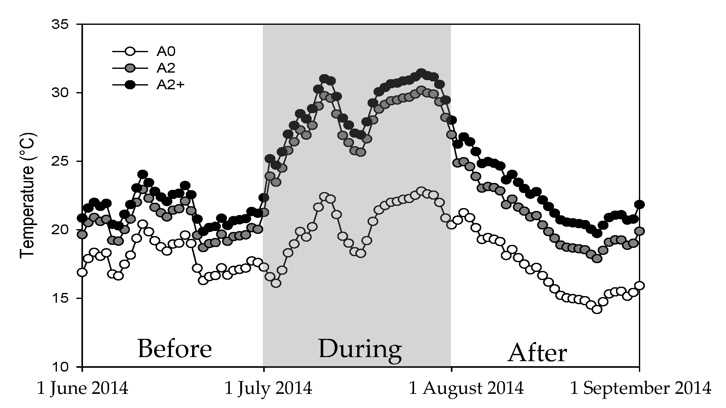
2.2. Heat Wave Treatment

The current experiment was undertaken from 1 June to end of August 2014. From 1 July to 1 August, a HW was created with an extra +5 °C increment of temperature in the heated A2 and A2+ scenarios (ca. +8 °C and +9.5 °C above ambient temperature, respectively), followed by a return to the normal heating. No heating was applied in the ambient temperature mesocosms. In the remaining text, the HW simulation experiment is referred to as “Before the HW”, “During the HW”, and “After the HW” (Figure 1).

2.3. Sampling and Laboratory Analysis

Temperature was measured at 30 min intervals and alkalinity was determined by end-point titration with 0.1 N HCl according to Gran [42] and measured once every 2 or 3 days. Sampling for determination of nutrients (TP and TN) and chlorophyll a (Chl-a) was done twice a week during the HW and otherwise once a week. Standard methods were used for chemical variables [43]. Chl-a was estimated using ethanol extraction [44].
Zooplankton samples were taken on 26 and 30 June representing the before period of the HW, 2, 7, 14, 21, and 28 July (the HW period) and 4 and 28 August (the after period of the HW). Sampling was conducted with a 1 m long tube sampler (covering the whole water column) at 6 randomly selected sites and pooled. Eight liters of the composite sample were filtered through a 50 µm mesh and preserved in 4% Lugol’s solution for further analysis. Identification of all zooplankton taxa was carried out to genus or taxon level, whenever possible. Copepods were separated into cyclopoids and calanoids (including adults and copepodites) and nauplii (without further determination). Counting and identification of the samples were done using a stereomicroscope (Leica M125) for cladocerans and copepods and an inverted microscope (Leica DMI 4000 B) for rotifers and nauplii. We measured the body size of about 25 individuals of each taxon, when possible, and calculated the body weight from length-weight allometric relationships [45,46,47,48]. For rotifers, we used the geometric formulae suggested by Ruttner-Kolisko [49]. We calculated biovolumes and converted them to dry weight according to Dumont et al. [45], Ruttner-Kolisko [49] and Malley et al. [50]. Phytoplankton samples were taken with the same frequency as the zooplankton samples, identification was undertaken to at least genus level, followed by counting and conversion to biomass as described in Filiz et al. [51]. Macrophyte abundance was quantified as percent volume of the water column inhabited by plants (plant volume inhabited (PVI, %)). Percentage cover and height of the submerged plants were assessed, allowing estimation of the proportion of the water column occupied by submerged plants (for further details see Davidson et al. [52]).

2.4. Stability Analyses

Following the procedure in Hillebrand et al. [53], we measured resistance in zooplankton total biomass as functional stability during the disturbance. Considering the fact that our HW lasted a month (extended pulse disturbance), we included data from all five samples taken during the HW for the resistance analysis. Resistance (as the differences between disturbed and undisturbed communities) was calculated by log response ratio (LRR). LRR was applied to zooplankton total biomass between undisturbed (just before the HW) and disturbed (during the HW) mesocosms within the treatments. Slope of regression over time was calculated in R with the ‘lm’ function in the “stats” package [54] to see the change in resistance during the time that HW was applied. One sample t-test was used to check if there was a significant difference between the benchmarks and the functional stability (resistance) with the ‘t.test’ function in R [53,54]. In order to gain benchmark values for resistance, instead of 0 (referring to no change between the mesocosms), we used data from just before the HW. Since the treatments (A2 and A2+) had already been held at higher than ambient temperatures for 11 years prior to the HW, the initial conditions between the treatments and their control were not the same. We did not calculate recovery or resilience since the treatments were resistant to the disturbance.

2.5. Statistical Analyses

Taxon diversity was calculated from the abundance data according to the Shannon-Wiener Index (H) and Pielou’s evenness (J) using the “vegan” package [55]. Taxon richness was an expression of the total number of all determined taxa, excluding nauplii and copepodites. Size diversity (μ) was computed based on the Shannon diversity index adapted for a continuous variable, such as body size, following the methodology described in Quintana et al. [56]. High size diversity implies a wide size range and/or similar proportions of the different sizes [56,57,58,59]. A basic taxonomic grouping separating Cladocera, Copepoda, and Rotifera was done. This was followed by functional grouping according to Barnett et al. [60], Obertegger and Manca [61], and Gutierrez et al. [62], based on zooplankton feeding strategies, predator avoidance, and growth (8 groups including benthic filter feeders (Ilyocryptus sordidus) filtering anomopoda (Simocephalus vetulus), filtering scrapers (Alona sp. and Chydoridae), selective filter feeders (Bosmina longirostris), microphagous carnivore (Cyclopoidea), microphagous detritivore (Harpacticoidea), raptorial (Ascomorpha, Asplanchna, Collotheca, Gastropus, Polyarthra, Synchaeta and Trichocerca), and, finally, microphages (Brachionus and Euchlanis, Filinia, Keratella, Lecane, Notholca, Testudinella and Trichotria). Functional group diversity (FGD) and functional group evenness (FGE) were then also calculated according to Shannon-Wiener Index (H) and Pielou’s evenness (J), respectively.
Linear mixed models (LMMs) were used to determine the treatment effects on zooplankton biomass, taxonomic composition, community parameters and size structure using the ‘lmer’ function in the “lme4” package in R [63]. Sampling date was used as a random effect, and the fixed effects were different temperatures (A2, A2+) and nutrient treatments (LN, HN). Due to the limited number of samples before and after the HW, we ran separate analyses for the three periods (before, during, and after the HW). After running the models, residuals were checked by Shapiro-Wilk’s test (p > 0.05) for variance normality and homogeneity. If model residuals did not meet the normality assumption, box-cox transformation was applied to the dataset [64]. Interaction effects of different temperature and nutrient levels were selected according to the Akaike Information Criterion (AIC). If the models with interaction did not have lower AIC than those of the models without interaction, we did not take into consideration the interaction models in the analyses. To ascertain patterns between selected explanatory variables (temperature, PVI, Chl-a, alkalinity) and response variables (taxonomic grouping of zooplankton, taxon richness and evenness, and size diversity), co-inertia analysis (COI) was performed with the R package “ade4” [65] after testing for collinearity (8 being the accepted threshold, [66]) with the function ‘vifstep’ in the “usdm” package [67]. COI multivariate analysis can couple the two sets of data (here explanatory and response), following a Principle Component Analysis (PCA). Significance of the test acquired via free permutation test RV (number of random matching = 1000) [68,69].

3. Results

Daily average water temperatures for the three temperature scenarios from 1 June to 1 September are shown in Figure 1. Zooplankton sampling was undertaken from 26 June to 28 August. Before the HW in this time window, the average temperature was 17.3 ± 0.4 °C in A0, 19.8 ± 0.4 °C in A2, and 20.9 ± 0.4 °C in A2+. During the HW, the average temperature was 20.1 ± 2.2 °C in A0, 27.4 ± 2.2 °C in A2, and 28.7 ± 2.2 °C in A2+, and after the HW it was 18.2 ± 2.5 °C in A0, 21.9 ± 2.5 °C in A2, and 23.7 ± 2.5 °C in the A2+. During the zooplankton sampling period, average TP and TN concentrations were 0.404 ± 0.02 mg/L and 2.77 ± 0.13 mg/L, respectively, in HN, and 0.012 ± 0.001 mg/L and 0.284 ± 0.02 mg/L, respectively, in LN (see details in Table 1).
Major changes were observed in the PVI in some of the treatments during the experimental period (Figure 2). Linear regression revealed a significant decline with time in LN-A2 (p < 0.007, R2 = 0.25) and HN-A0 (p < 0.02, R2 = 0.19) and an increase in HN-A2 (p < 0.05, R2 = 0.27), the latter due to an increase in filamentous algae (data not shown). During the HW 9–14 July, fish kills were observed in HN-A2 and HN-A2+ between 9–14 July, averaging 4.5 and 12 indiv.), respectively in the two treatments, while no fish kills were observed in HN-A0 and all the LN mesocosms.

3.1. Community Structure before the Heat Wave

The initial zooplankton communities showed differences in structure between LN and HN, while there were only subtle differences among the temperature treatments within LN and HN. In LN, Simocephalus vetulus O.F. Müller 1776, Chydorus sphaericus O.F. Müller 1776, Euclanis sp., Brachionus spp., Trichotria sp., Monostyla sp., and nauplii contributed importantly to the total zooplankton biomass. In HN, Alona rectangula Sars, 1861, Chydrorus sphaericus O.F. Müller 1776, Filina longiseta Ehrenberg 1834, Keratella quadrata Müller 1786, Keratella cochlearis Gosse, 1851, and Brachionus spp. were the dominant taxa.
Rotifera biomass and zooplankton taxon richness were higher in HN and the biomass of large Cladocera, and also the grazing potential of zooplankton, expressed as the zooplankton: phytoplankton (Zoop: Phyto) biomass ratio, was lower in HN than in LN (Table 2, Figure 3 and Figure 4). HN was dominated by small-bodied zooplankton taxa (Table 2, Figure 3 and Figure 4), and the phytoplankton community largely consisted of Microcystis sp. [51]. HN also had lower FGD and FGE (Table 2, Figure 3).
Concerning the temperature effects, numbers of small Cladocera and small Copepoda were significantly higher in LN-A2 and taxon evenness higher in LN-A2+ than in LN-A0 (Table 2, Figure 3 and Figure 4). Temperature effects in HN were only seen for taxon richness in A2 (Table 2). Moreover, we found a significant negative interaction between nutrients and A2 warming for small Copepoda, and a significant positive interaction with A2+ warming for total zooplankton biomass (Table 2).

3.2. Community Structure during and after the Heat Wave

During and after the HW, the nutrient effect largely followed the pattern observed before the HW. However, during the HW, we also found a significantly lower size diversity as well as taxon evenness and taxon diversity in HN than in LN, and a higher biomass of small cladocerans (Table 2, Figure 3 and Figure 4). Considering the temperature effects, there was a significantly higher Rotifera biomass in LN-A2+ than in LN-A0, accompanied by a significantly lower size diversity, Zoop: Phyto biomass ratio, taxon evenness and diversity as well as lower FGD and FGE. In HN-A2+, the biomasses of total zooplankton and small Copepoda were significantly higher than in HN-A0 (Table 2). In addition, there was a positive nutrient and warming interaction in HN-A2+ for the biomass of total zooplankton, large Copepoda, small Copepoda, and the Zoop: Phyto ratio during the HW (Table 2).
The pattern for the nutrient effect after the HW largely followed the HW response, except that the nutrient effect on small cladocerans was no longer significant. Concerning temperature, the biomass of large Cladocera, size diversity, and taxon evenness were significantly lower in LN-A2+ than in LN-A0 (Table 2, Figure 3 and Figure 4). Taxon richness was significantly lower in both HN-A2 and HN-A2+ than in HN-A0. Moreover, the biomasses of total zooplankton and large Copepoda and the Zoop: Phyto biomass ratio were significantly higher in HN-A2+ than in HN-A0 (Table 2, Figure 3 and Figure 4). Interaction effects of nutrient and A2+ warming were significant for most variables, and there was a positive interaction effect for total zooplankton, large Cladocera, large Copepoda, and small Copepoda biomasses as well as for size diversity, the Zoop: Phyto biomass ratio, taxon evenness and taxon diversity. Taxon richness, however, was, negatively affected by the interaction between nutrient and A2+ warming (Table 2).

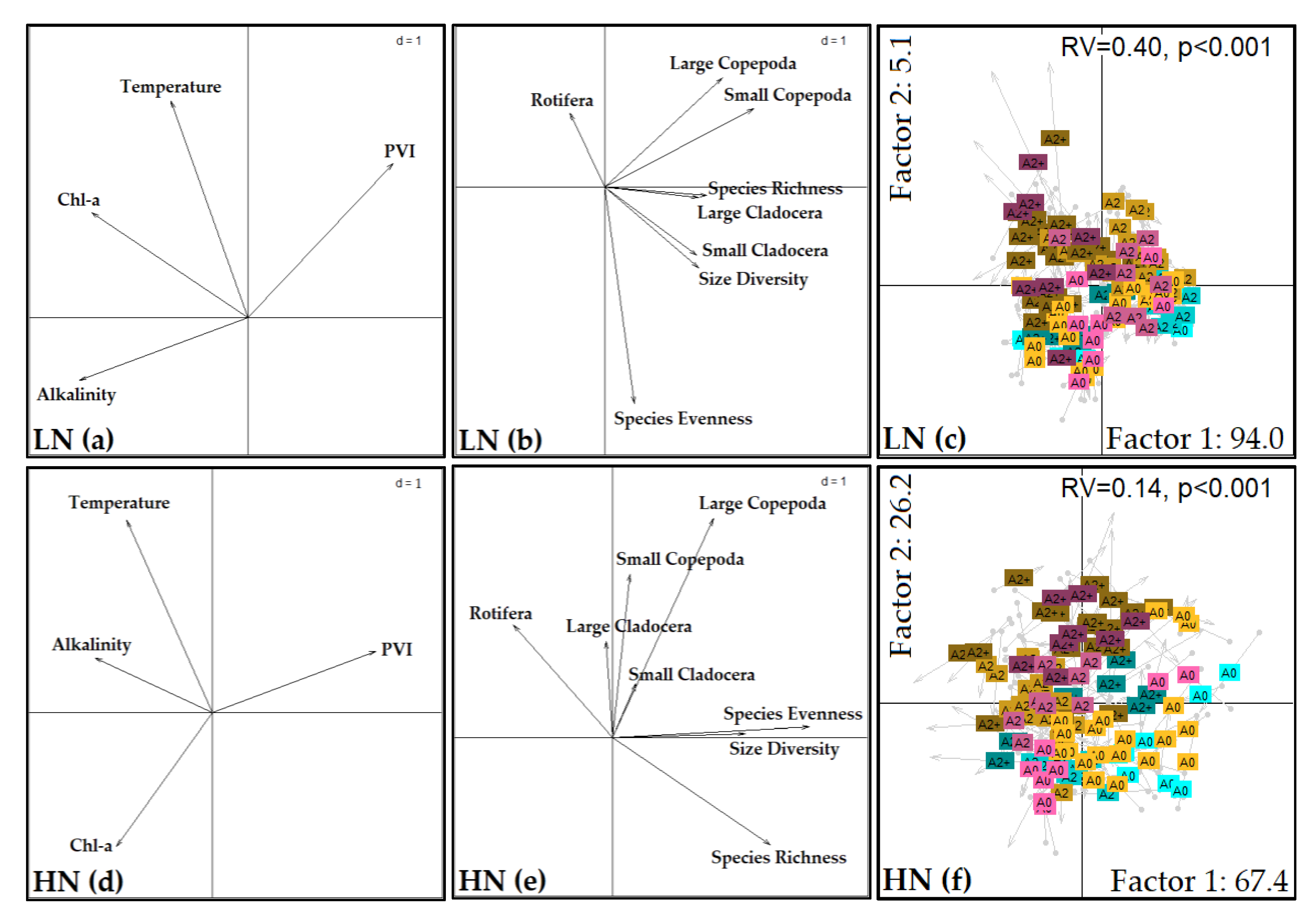
3.3. Co-Inertia Analysis

The relationships between the selected explanatory variables (temperature, Chl-a, alkalinity, PVI) and the zooplankton community response variables (large and small Cladocera and Copepoda, Rotifera, taxon richness and evenness of zooplankton, and size diversity) were further evaluated in the COI analyses, which were run separately for HN and LN. Dissolved oxygen was excluded in this analysis as it generally was high (super-saturation except for a short term period during a cooling event during the middle of the heat wave, see [70]). Significant relationships (p < 0.001) were found, with RV-coefficients of 0.40 and with the variance explained by the first two axes of 94.0% and 5.1% for LN; for HN, RV-coefficients were much lower, 0.14, as was the variance explained by the first two axes, namely 67.4% and 26.2% (Figure 5). In Figure 5, panels (c) and (f) show the concordance between the explanatory and response variables and the distributions before, during, and after the HW are displayed by color gradients. The relative location of samples within the two datasets (explanatory and response) are presented by arrows in Figure 5, panels (c) and (f). Even though the grouping of the treatments that was exposed to HW (A2 and A2+ during the HW) was not clearly distinguishable from the others for either LN or HN, these treatments were grouped with A2 and A2+ from after the HW in LN (Figure 5c).
In the LN ordination plots, PVI was an important explanatory variable, not least of all for large and small Copepoda, which were strongly associated with PVI. Large Cladocera and taxon richness, small Cladocera and size diversity were also associated with PVI and/or low Chl-a and with temperature. Taxon evenness was negatively associated with temperature, while Rotifera were positively associated with temperature and Chl-a (Figure 5a,b). The pattern in HN followed that in LN, although the relationship was weaker.

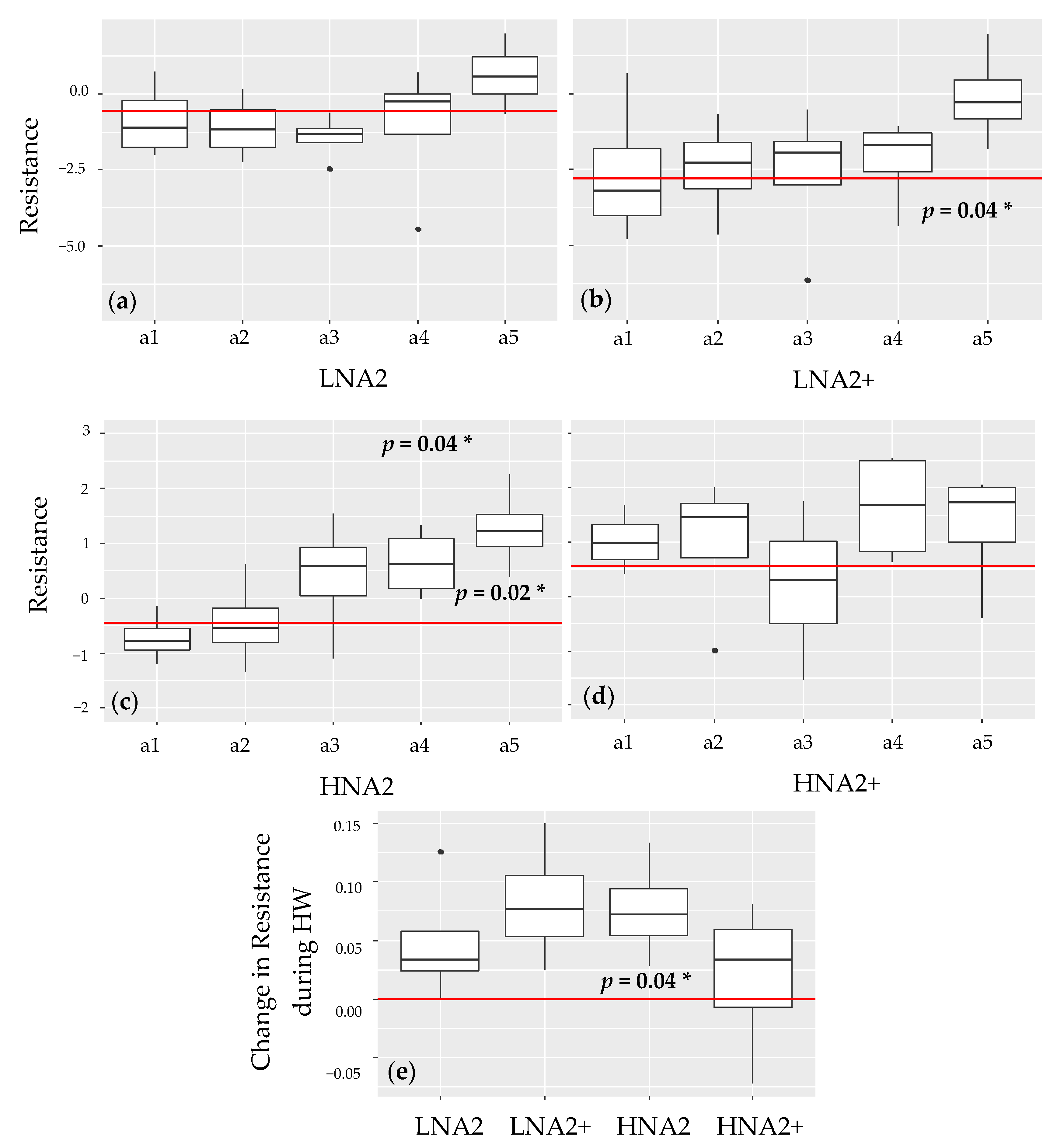
3.4. Stability Analyses

The stability analysis revealed no differences compared to the benchmark during the HW in LN-A2 (thus showing resistance to the HW disturbance), whereas LN-A2+ deviated, showed less resistance, as from the second week of the HW and significantly so in the last week of sampling (Figure 6a,b). HN-A2 similarly deviated from the benchmark after the third week, with a significant change occurring in the fourth and fifth weeks of the HW, thus became less resistant. HN-A2+ showed no significant change from the benchmark but a similar trend as in HN-A2 (Figure 6c,d), thus remaining resistant. The slope of change tended to be positive for all treatments during the HW, but only significantly so for HN-A2 (Figure 6e).

4. Discussion

Our results clearly showed that the effects of eutrophication on the zooplankton community composition and abundance were much larger than those observed for the temperature treatments in all three periods (before, during, and after the HW), supporting our first hypothesis. This concurs with a recent cross-system analysis from mesocosms and lakes, finding an overall stronger effects of nutrients than of temperature on various biota [33]. However, our results may also reflect the fact that the variation in nutrients far exceeded the variation in temperature, even though the temperature increase was relatively large. The COI analysis, moreover, revealed that PVI was a key explanatory variable in LN, in particular for large and small Copepoda, which were strongly associated with PVI (Figure 2 and Figure 5). Large Cladocera, taxon richness, small Cladocera, and size diversity were also associated with PVI and/or low Chl-a. It is well established that macrophytes act both as a habitat and a refuge against fish predation, and the biofilm on the plant surface provides food for some cladocerans and copepods (e.g., [71,72]). Although the effect of PVI in HN largely followed the pattern in LN, it was weaker, which is to be expected as the PVI was overall much lower in HN, except for HN-A0 (Figure 2) and in eutrophic lakes in general [16].
We found no major difference in total zooplankton biomass among the treatments, it being higher only in the HN mesocosms heated to the A2+ warming scenario during and after the HW. We would have expected (Hypothesis 2) an increase in zooplankton biomass from LN to HN conditions, as typically seen in shallow Danish lakes [73]. In HN, fish have been allowed to breed freely since 2006, which likely has created a high, though variable, predation pressure on the zooplankton [20] and a shift to Rotifera dominance as observed in eutrophic shallow Danish lakes [73]. High fish predation is known to alter the zooplankton community in favor of rotifers [73,74] and this may explain the overall lower biomass and the lower Zoop: Phyto biomass ratio in HN compared with LN [35]. Our mesocosms were too small to have also piscivorous fish included, which may have contributed to the modest effect of nutrients on the zooplankton biomass (Hypothesis 2). However, the deteriorated food quality caused by cyanobacteria dominance in these mesocosms [51] may also have been a contributory factor [75,76,77].
Before the HW, taxon diversity, evenness, and size diversity were not affected by nutrients. Taxon richness, however, was higher, and functional group diversity and evenness were lower in HN. This pattern was also found both during and after the HW, but in addition taxon diversity, evenness, and size diversity were lower in HN than in LN, emphasizing the effect of nutrients on community structure and function especially exposed to the HW (Hypotheses 1, 3 and 4).
Prior to the HW, we found only few significant temperature treatment effects. Small Cladocera and small Copepoda were higher in LN-A2 and large Cladocera lower in LN-A2+ compared with the controls (Table 2), suggesting a higher predation pressure with warming reflects size-selective predation (Hypothesis 3). Such a temperature effect on predation is observed both in cross-system mesocosm studies and in field data [23,26]. We also found a significantly lower taxon richness in
HN-A2 and an increase in taxon evenness in LN-A2+ compared with their respective controls, but otherwise there was no observable warming effect.
During the HW, major temperature treatment effects were found in LN-A2+ (higher rotifer biomass; lower taxon diversity, taxon evenness, size diversity, FGD, FGE, and Zoop: Phyto ratio), and these changes persisted for some of the variables after the HW (Table 2). The higher contribution of rotifers and higher Zoop: Phyto ratio suggesting increasing predation [19] likely reflect the higher temperature, as we did not find any significant reduction in PVI in LN-A2+ (Figure 2), which otherwise could have led to higher predation risk [71].
Furthermore, HN-A2+ showed a different pattern during and after the HW from the before period, having higher total zooplankton biomass (during and after the HW) and higher biomass of large cladocerans and Zoop: Phyto ratio than HN-A0. Contrary to the findings in LN, the changes in HN-A2+ indicate less fish predation. Accordingly, we observed fish kill in HN-A2 and HN-A2+, 9–14 days into the HW, but being much larger in HN-A2+ (Hypothesis 3). The remaining fish population may also have suffered warming effects as Moran et al. [78] experimentally demonstrated a negative effect of warming on three-spined stickleback survival and reproduction, with a 60% reduction of stickleback biomass at a temperature increase of 4 °C above ambient summer temperatures. Moreover, in their experiment the combined effect of heating and enhanced nutrient loading led to a further stickleback population decline, attributed to indirect effects of warming such as low oxygen concentrations. Unfortunately, we have no fish data from this study (apart from data on fish kill), but an earlier study by Šorf et al. [79] in the same mesocosms revealed that the lowest adult stickleback catch per unit effort (CPUE) and the highest recruitment occurred in the unheated HN mesocosms, suggesting that stickleback recruitment declined at the higher temperatures. Concurring with these results, Mehlis and Bakker [80] found that while less sperm fertilized more eggs at higher temperature (25 °C), the overall percentage of motile sperm significantly decreased. A negative effect on fish due to HW might, therefore, partly explain why the zooplankton biomass increased and crustaceans became more abundant in HN-A2+ during and after the HW (Hypothesis 3), while no such effect is to be expected in LN due presence of only one male stickleback.
The overall modest effect of temperature (apart from the highest temperature, A2+) concurs with results from a series of mesocosm experiments conducted in Liverpool, UK (e.g., [34,81]) as well as an earlier study of zooplankton in our mesocosms [20]. From the Liverpool experiment, McKee et al. [81] concluded that the effect of increased temperature caused by global warming is not expected to significantly alter ecosystem functional structures and processes during the next century. However, microevolution may be a contributing factor, considering that the zooplankton communities of our mesocosms have been facing warming for 11 years prior to this experiment. This is supported by a study in our mesocosm systems by Van Doorslaer et al. [82], which showed rapid (within a year) microevolution of S. vetulus. They found that clones exposed for 1 year to the A2+ treatment had about a five times higher survival rate at 26 °C than that of clones exposed to the ambient regime. Moreover, age at first reproduction and offspring numbers were affected, and the authors concluded that the S. vetulus populations would probably not be able to maintain themselves under global warming. Microevolution may thus help buffer changes in community structure under global warming. Moreover, although some zooplankton taxa are considered to be sensitive to temperature changes [83], cosmopolitan taxa such as C. sphaericus, A. rectangula, B. calcyflorus, and K. quadrata dominated the zooplankton community in the high-nutrient mesocosms [84,85,86,87,88], which may explain the resistance to increased temperature. Additionally, C. sphaericus was the most abundant Cladocera taxon in the HN-A2+ mesocosms and has an advantage by having a short egg development time, allowing fast development of populations under favorable environmental conditions [89]. Moreover, several previous experimental studies have shown tolerance of selected cladocerans to temperatures up to 30 °C [90,91]. An investigation by Donze [92] demonstrated an effect of heat on the survival of cladocerans at 30 °C with 0% mortality, while at 34 °C mortality was around 75%. The temperature variation in our mesocosms did not exceed these temperatures during the experimental period (Figure 1), and cladocerans might, therefore, have shown resistance to the heating scenarios (A2 and A2+ according to IPCC), though heat-shock proteins in zooplankton may somehow prevent cellular damage and constitute a molecular defense mechanism against all kinds of stressors [93,94].
The resistance analysis and the change in the resistance during HW revealed that all the treatments tended to have over-performance (i.e., higher biomass than in the benchmark for a given treatment) by the end of the HW disturbance (Figure 6a,d), which may be explained by the increased resource availability [51]. However, our results mostly showed insignificant changes in the different treatments, indicating overall high resistance to the HW disturbance. In LN-A2+ and HN-A2, however, the resistance in the beginning of the HW did not last until the end of the HW period.
We acknowledge that our study has some limitations regarding elucidation of the HW effect, as the HW was run without true controls to account for seasonal effects. Differences observed among the three periods (before, during, and after the HW) should therefore be interpreted with caution. However, the rather modest effect of the HW, despite a 5 °C increase in temperature resulting in, respectively, an 8 and 9.5 °C increase above the temperature in the ambient mesocosm, suggests that our conclusion of high nutrient but lower temperature and HW effects is valid. However, fish kill in HN-A2 and not least in HN-A2+ enhanced the effect of the HW. Modest effects of the HW were also found for phytoplankton in the same experiment [51], whereas temperature changes had a substantial effect on the biomass of bacterioplankton, heterotrophic flagellates, ciliates [95], and macrophytes [13], oxygen metabolism (gross ecosystem production and ecosystem respiration), and bacterioplankton production [96], as well as on greenhouse gases dynamics [70]. These results suggest that microbial communities and ecosystem processes are more sensitive to short-term HWs than the larger-bodied and more slow-growing organisms, such as zooplankton, which are likely to exhibit a delayed or weak response, unless a major fish kill occurs.

5. Conclusions

Our results indicate that the nutrients’ effect on zooplankton community composition was much higher than that of temperature for three periods before, during, and after the heat wave (HW). They further showed that the HW had only modest effects on the zooplankton community. Our results indicate that a rise in the number of HWs and global temperatures may potentially weaken the capacity of maintaining or establishing a clear water state by shifting the zooplankton community towards dominance of small-sized taxa with a lower grazing potential, at least in systems that lack piscivorous fish, provided that the zooplanktivorous fish present are not subjected to fish kill at the higher temperature of HWs as seen in the HN-high temperature mesocosms in our experiment. Reduction of the external nutrient loading can, therefore, somehow compensate for the effect of warming due to climate change and help prevent fish kills during heat waves.

Author Contributions

Conceptualization, M.B. and E.J.; Data curation, U.I., N.F. and B.Ö.; Formal analysis, U.I. and N.F.; Funding acquisition, M.B. and E.J.; Investigation, U.I., N.F., Y.C. and É.M.N.; Methodology, E.J.; Project administration, E.J.; Resources, M.B. and E.J.; Supervision, M.B. and E.J.; Visualization, U.I. and N.F.; Writing – original draft, U.I., N.F., M.B. and E.J.; Writing – review & editing, U.I., N.F., Y.C., T.L.L, T.A.D., M.S., Ü.N.T., M.B. and E.J. All authors have read and agreed to the published version of the manuscript.

Funding

This research was funded by EU 7th Framework MARS Project, Grant/Award Number: 603378; Türkiye Bilimsel ve Teknolojik Araştırma Kurumu (TÜBİTAK)—BİDEB, Grant/Award number: 2211E and TÜBİTAK-2232, CLIM-SALTLAKES Project, Grant/Award number: 118C250.

Acknowledgments

We thank the staff at Aarhus University, Silkeborg, for technical assistance with field and lab work and A.M. Poulsen for manuscript edition.

Conflicts of Interest

The authors declare no conflict of interest.

References

  1. Shiklomanov, I. World Fresh Water Resources. In Water in Crisis a Guide to the World’s Fresh Water Resources; Gleick, P., Ed.; Oxford University Press: Oxford, NY, USA, 1993; pp. 13–24. [Google Scholar]
  2. Verpoorter, C.; Kutser, T.; Seekell, D.A.; Tranvik, L.J. A Global Inventory of Lakes Based on High-Resolution Satellite Imagery. Geophys. Res. Lett. 2014, 41, 6396–6402. [Google Scholar] [CrossRef]
  3. Brönmark, C.; Hansson, L.A. The Biology of Lakes and Ponds, 3rd ed.; Oxford University Press: Oxford, UK, 2017. [Google Scholar] [CrossRef]
  4. Dudgeon, D.; Arthington, A.H.; Gessner, M.O.; Kawabata, Z.-I.; Knowler, D.J.; Lévêque, C.; Naiman, R.J.; Prieur-Richard, A.-H.; Soto, D.; Stiassny, M.L.J.; et al. Freshwater Biodiversity: Importance, Threats, Status and Conservation Challenges. Biol. Rev. Camb. Philos. Soc. 2006, 81, 163–182. [Google Scholar] [CrossRef]
  5. Jeppesen, E.; Kronvang, B.; Meerhoff, M.; Søndergaard, M.; Hansen, K.M.; Andersen, H.E.; Lauridsen, T.L.; Liboriussen, L.; Beklioğlu, M.; Özen, A.; et al. Climate Change Effects on Runoff, Catchment Phosphorus Loading and Lake Ecological State, and Potential Adaptations. J. Environ. Qual. 2009, 38, 1930–1941. [Google Scholar] [CrossRef]
  6. Moss, B. Allied Attack: Climate Change and Eutrophication. Inland Waters 2011, 1, 101–105. [Google Scholar] [CrossRef] [Green Version]
  7. IPCC. Climate Change 2001: The Scientific Basis; Contribution of Working Group I to the Third Assessment Report of the Intergovernmental Panel on Climate, Change; Houghton, J.T., Ding, Y., Griggs, D.J., Noguer, M., Van der Linden, P.J., Dai, X., Maskell, K., Johnson, C.A., Eds.; Cambridge University Press: Cambridge, UK; New York, NY, USA, 2001. [Google Scholar] [CrossRef]
  8. Meehl, G.; Tebaldi, C. More Intense, More Frequent, and Longer Lasting Heat Waves in the 21st Century. Science 2004, 305, 994–997. [Google Scholar] [CrossRef] [PubMed] [Green Version]
  9. IPCC. Climate Change 2014: Synthesis Report; Contribution of Working Groups I, II and III to the Fifth Assessment Report of the Intergovernmental Panel on Climate Change; IPCC: Geneva, Switzerland, 2014. [Google Scholar]
  10. Christidis, N.; Jones, G.S.; Stott, P.A. Dramatically Increasing Chance of Extremely Hot Summers since the 2003 European Heatwave. Nat. Clim. Chang. 2015, 5, 46–50. [Google Scholar] [CrossRef]
  11. Jankowski, T.; Livingstone, D.M.; Bührer, H.; Forster, R.; Niederhauser, P. Consequences of the 2003 European Heat Wave for Lake Temperature Profiles, Thermal Stability, and Hypolimnetic Oxygen Depletion: Implications for a Warmer World. Limnol. Oceanogr. 2006, 51, 815–819. [Google Scholar] [CrossRef] [Green Version]
  12. Huber, V.; Adrian, R.; Gerten, D. A Matter of Timing: Heat Wave Impact on Crustacean Zooplankton. Freshw. Biol. 2010, 55, 1769–1779. [Google Scholar] [CrossRef]
  13. Cao, Y.; Neif, É.M.; Li, W.; Coppens, J.; Filiz, N.; Lauridsen, T.L.; Davidson, T.A.; Søndergaard, M.; Jeppesen, E. Heat Wave Effects on Biomass and Vegetative Growth of Macrophytes after Long-Term Adaptation to Different Temperatures: A Mesocosm Study. Clim. Res. 2015, 66, 265–274. [Google Scholar] [CrossRef]
  14. Woodward, G.; Bonada, N.; Brown, L.E.; Death, R.G.; Durance, I.; Gray, C.; Hladyz, S.; Ledger, M.E.; Milner, A.M.; Ormerod, S.J.; et al. The Effects of Climatic Fluctuations and Extreme Events on Running Water Ecosystems. Philos. Trans. R. Soc. B 2016, 371, 20150274. [Google Scholar] [CrossRef] [PubMed] [Green Version]
  15. Moss, B. Engineering and Biological Approaches to the Restoration from Eutrophication of Shallow Lakes in Which Aquatic Plant Communities Are Important Components. Hydrobiologia 1990, 200–201, 367–377. [Google Scholar] [CrossRef]
  16. Scheffer, M.; Hosper, S.H.; Meijer, M.L.; Moss, B.; Jeppesen, E. Alternative Equilibria in Shallow Lakes. Trends Ecol. Evol. 1993, 8, 275–279. [Google Scholar] [CrossRef]
  17. Jeppesen, E.; Søndergaard, M.; Søndergaard, M.; Christoffersen, K. The Structuring Role of Submerged Macrophytes in Lakes; Springer: New York, NY, USA; Berlin/Heidelberg, Germany, 1998. [Google Scholar]
  18. Van De Waal, D.B.; Verschoor, A.M.; Verspagen, J.M.H.; Van Donk, E.; Huisman, J. Climate-Driven Changes in the Ecological Stoichiometry of Aquatic Ecosystems. Front. Ecol. Environ. 2010, 8, 145–152. [Google Scholar] [CrossRef] [Green Version]
  19. Jeppesen, E.; Nõges, P.; Davidson, T.A.; Haberman, J.; Nõges, T.; Blank, K.; Lauridsen, T.L.; Søndergaard, M.; Sayer, C.; Laugaste, R.; et al. Zooplankton as Indicators in Lakes: A Scientific-Based Plea for Including Zooplankton in the Ecological Quality Assessment of Lakes According to the European Water Framework Directive (WFD). Hydrobiologia 2011, 676, 279–297. [Google Scholar] [CrossRef]
  20. Šorf, M.; Davidson, T.A.; Brucet, S.; Menezes, R.F.; Søndergaard, M.; Lauridsen, T.L.; Landkildehus, F.; Liboriussen, L.; Jeppesen, E. Zooplankton Response to Climate Warming: A Mesocosm Experiment at Contrasting Temperatures and Nutrient Levels. Hydrobiologia 2015, 742, 185–203. [Google Scholar] [CrossRef]
  21. Teixeira-De Mello, F.; Meerhoff, M.; Pekcan-Hekim, Z.; Jeppesen, E. Substantial Differences in Littoral Fish Community Structure and Dynamics in Subtropical and Temperate Shallow Lakes. Freshw. Biol. 2009, 54, 1202–1215. [Google Scholar] [CrossRef]
  22. Jeppesen, E.; Meerhoff, M.; Holmgren, K.; González-Bergonzoni, I.; Teixeira-de Mello, F.; Declerck, S.A.J.; De Meester, L.; Søndergaard, M.; Lauridsen, T.L.; Bjerring, R.; et al. Impacts of Climate Warming on Lake Fish Community Structure and Potential Effects on Ecosystem Function. Hydrobiologia 2010, 646, 73–90. [Google Scholar] [CrossRef]
  23. Iglesias, C.; Mazzeo, N.; Meerhoff, M.; Lacerot, G.; Clemente, J.M.; Scasso, F.; Kruk, C.; Goyenola, G.; García-Alonso, J.; Amsinck, S.L.; et al. High Predation Is of Key Importance for Dominance of Small-Bodied Zooplankton in Warm Shallow Lakes: Evidence from Lakes, Fish Exclosures and Surface Sediments. Hydrobiologia 2011, 667, 133–147. [Google Scholar] [CrossRef]
  24. Strecker, A.L.; Cobb, T.P.; Vinebrooke, R.D. Effects of Experimental Greenhouse Warming on Phytoplankton and Zooplankton Communities in Fishless Alpine Ponds. Limnol. Oceanogr. 2004, 49, 1182–1190. [Google Scholar] [CrossRef]
  25. Kosten, S.; Huszar, V.L.M.; Bécares, E.; Costa, L.S.; van Donk, E.; Hansson, L.A.; Jeppesen, E.; Kruk, C.; Lacerot, G.; Mazzeo, N.; et al. Warmer Climates Boost Cyanobacterial Dominance in Shallow Lakes. Glob. Chang. Biol. 2012, 18, 118–126. [Google Scholar] [CrossRef]
  26. Tavşanoğlu, Ü.N.; Šorf, M.; Stefanidis, K.; Brucet, S.; Türkan, S.; Agasild, H.; Baho, D.L.; Scharfenberger, U.; Hejzlar, J.; Papastergiadou, E.; et al. Effects of Nutrient and Water Level Changes on the Composition and Size Structure of Zooplankton Communities in Shallow Lakes under Different Climatic Conditions: A Pan-European Mesocosm Experiment. Aquat. Ecol. 2017, 1–17. [Google Scholar] [CrossRef]
  27. Brown, J.H.; Gillooly, J.F.; Allen, A.P.; Savage, V.M.; West, G.B. Toward a Metabolic Theory of Ecology. Ecology 2004, 85, 1771–1789. [Google Scholar] [CrossRef]
  28. Daufresne, M.; Lengfellner, K.; Sommer, U. Global Warming Benefits the Small in Aquatic Ecosystems. Proc. Natl. Acad. Sci. USA 2009, 106, 12788–12793. [Google Scholar] [CrossRef] [Green Version]
  29. Gardner, J.L.; Peters, A.; Kearney, M.R.; Joseph, L.; Heinsohn, R. Declining Body Size: A Third Universal Response to Warming? Trends Ecol. Evol. 2011, 26, 285–291. [Google Scholar] [CrossRef] [PubMed]
  30. Brucet, S.; Boix, D.; Quintana, X.D.; Jensen, E.; Nathansen, L.W.; Trochine, C.; Meerhoff, M.; Gascón, S.; Jeppesen, E.; Gascon, S.; et al. Factors Influencing Zooplankton Size Structure at Contrasting Temperatures in Coastal Shallow Lakes: Implications for Effects of Climate Change. Limnol. Oceanogr. 2010, 55, 1697–1711. [Google Scholar] [CrossRef] [Green Version]
  31. Forster, J.; Hirst, A.G.; Atkinson, D. Warming-Induced Reductions in Body Size Are Greater in Aquatic than Terrestrial Species. Proc. Natl. Acad. Sci. USA 2012, 109, 19310–19314. [Google Scholar] [CrossRef] [Green Version]
  32. Havens, K.E.; Pinto-Coelho, R.M.; Beklioğlu, M.; Christoffersen, K.S.; Jeppesen, E.; Lauridsen, T.L.; Mazumder, A.; Méthot, G.; Alloul, B.P.; Tavşanoğlu, U.N.; et al. Temperature Effects on Body Size of Freshwater Crustacean Zooplankton from Greenland to the Tropics. Hydrobiologia 2015, 743, 27–35. [Google Scholar] [CrossRef] [Green Version]
  33. Birk, S.; Chapman, D.; Carvalho, L.; Spears, B.M.; Andersen, H.E.; Argillier, C.; Auer, S.; Baattrup-Pedersen, A.; Banin, L.; Beklioğlu, M.; et al. Impacts of Multiple Stressors on Freshwater Biota across Spatial Scales and Ecosystems. Nat. Ecol. Evol. 2020, 4, 1060–1068. [Google Scholar] [CrossRef]
  34. Moss, B.; Mckee, D.; Atkinson, D.; Collings, S.E.; Eaton, J.W.; Gill, A.B.; Harvey, I.; Hatton, K.; Heyes, T.; Wilson, D. How Important Is Climate? Effects of Warming, Nutrient Addition and Fish on Phytoplankton in Shallow Lake Microcosms. J. Appl. Ecol. 2003, 40, 782–792. [Google Scholar] [CrossRef] [Green Version]
  35. Jeppesen, E.; Kronvang, B.; Jørgensen, T.B.; Larsen, S.E.; Andersen, H.E.; Søndergaard, M.; Liboriussen, L.; Bjerring, R.; Johansson, L.S.; Trolle, D.; et al. Recent Climate-Induced Changes in Freshwaters in Denmark. In Climatic Change and Global Warming of Inland Waters: Impacts and Mitigation for Ecosystems and Societies; Goldman, C.R., Kumagai, M., Robarts, R.D., Eds.; Wiley-Blackwell: Hoboken, NJ, USA, 2012. [Google Scholar] [CrossRef]
  36. Schindler, D.W. The Cumulative Effects of Climate Warming and Other Human Stresses on Canadian Freshwaters in the New Millennium. Can. J. Fish. Aquat. Sci. 2001, 58, 18–29. [Google Scholar] [CrossRef]
  37. Woodward, G.; Perkins, D.M.; Brown, L.E. Climate Change and Freshwater Ecosystems: Impacts across Multiple Levels of Organization. Philos. Trans. R. Soc. Lond. B Biol. Sci. 2010, 365, 2093–2106. [Google Scholar] [CrossRef] [PubMed] [Green Version]
  38. Liboriussen, L.; Landkildehus, F.; Meerhoff, M.; Bramm, M.E.; Søndergaard, M.; Christoffersen, K.; Richardson, K.; Søndergaard, M.; Lauridsen, T.L.; Jeppesen, E. Global Warming: Design of a Flow-through Shallow Lake Mesocosm Climate Experiment. Limnol. Oceanogr. Methods 2005, 3, 1–9. [Google Scholar] [CrossRef]
  39. Jeppesen, E.; Moss, B.; Bennion, H.; Carvalho, L.; Demeester, L.; Feuchtmayr, H.; Friberg, N.; Gessner, M.O.; Hefting, M.; Lauridsen, T.L.; et al. Interaction of Climate Change and Eutrophication. In Climate Change Impacts on Freshwater Ecosystems; Kernan, M., Battarbee R., W., Moss, B., Eds.; Wiley-Blackwell: Hoboken, NJ, USA, 2010. [Google Scholar] [CrossRef] [Green Version]
  40. IPCC. Climate Change 2007: Synthesis Report; Contribution of Working Groups I, II and III to the Fourth Assessment Report of the Intergovernmental Panel on Climate Change. Core Writing Team; Pachauri, R.K., Reisinger, A., Eds.; IPCC: Geneva, Switzerland, 2007; 104p. [Google Scholar]
  41. Landkildehus, F.M.; Søndergaard, M.; Beklioglu, R.; Adrian, D.G.; Angeler, J.; Hejzlar, E.; Papastergiadou, P.; Zingel, A.; İdil Çakiroğlu, U.; Scharfenberger, S.; et al. Jeppesen. Climate change effects on shallow lakes: Design and preliminary results of a cross-European climate gradient mesocosm experiment. Estonian J. Ecol. 2014, 63, 71–89. [Google Scholar] [CrossRef] [Green Version]
  42. Gran, G. Determination of the Equivalence Point in Potentiometric Titrations. Part II. Analyst 1952, 77, 661–671. [Google Scholar] [CrossRef]
  43. Søndergaard, M.; Jeppesen, E.; Jensen, J.P.; Amsinck, S.L. Water Framework Directive: Ecological Classification of Danish Lakes. J. Appl. Ecol. 2005, 42, 616–629. [Google Scholar] [CrossRef]
  44. Jespersen, A.; Christoffersen, K. Measurements of Chlorophyll―A from Phytoplankton Using Ethanol as Extraction Solvent. Arch. Hydrobiol. 1987, 109, 445–454. [Google Scholar]
  45. Dumont, H.J.; Van de Velde, I.; Dumont, S. The Dry Weight Estimate of Biomass in a Selection of Cladocera, Copepoda and Rotifera from the Plankton, Periphyton and Benthos of Continental Waters. Oecologia 1975, 19, 75–79. [Google Scholar] [CrossRef]
  46. Bottrell, H.H. A Review of Some Problems in Zooplankton Production Studies. Nor. J. Zool. 1976, 24, 419–456. [Google Scholar]
  47. McCauley, E. The Estimation of the Abundance and Biomass of Zooplankton in Samples. In A Manual on Methods for the Assessment of Secondary Productivity in Fresh Waters; Downing, J.A., Rigler, F.H., Eds.; Blackwell: Oxford, UK, 1984; pp. 228–265. [Google Scholar]
  48. Michaloudi, E. Dry Weights of the Zooplankton of Lake Mikri Prespa (Macedonia, Greece). Belgian J. Zool. 2005, 135, 223–227. [Google Scholar]
  49. Ruttner-Kolisko, A. Sugestions for Biomass Calculations of Plankton Rotifers. Arch. Hydrobiol. Belh. Ergebn. Limnol. 1977, 135, 223. [Google Scholar]
  50. Malley, D.F. Range of Variation in Estimates of Dry Weight for Planktonic Crustacea and Rotifera from Temperate North American Lakes; Canada Department of Fisheries and Oceans Central and Arctic Region: Sarnia, ON, USA, 1989.
  51. Filiz, N.; Işkın, U.; Beklioǧlu, M.; Öğlü, B.; Cao, Y.; Davidson, T.A.; Søndergaard, M.; Lauridsen, T.L.; Jeppesen, E. Phytoplankton Community Response to Nutrients, Temperature, and a Heat Wave in Shallow Lakes: An Experimental Approach. Water 2020, 12, 3394. [Google Scholar] [CrossRef]
  52. Davidson, T.A.; Audet, J.; Svenning, J.C.; Lauridsen, T.L.; Søndergaard, M.; Landkildehus, F.; Larsen, S.E.; Jeppesen, E. Eutrophication Effects on Greenhouse Gas Fluxes from Shallow-Lake Mesocosms Override Those of Climate Warming. Glob. Chang. Biol. 2015, 21, 4449–4463. [Google Scholar] [CrossRef] [PubMed]
  53. Hillebrand, H.; Langenheder, S.; Lebret, K.; Lindström, E.; Östman, Ö.; Striebel, M. Decomposing Multiple Dimensions of Stability in Global Change Experiments. Ecol. Lett. 2018, 21, 21–30. [Google Scholar] [CrossRef] [PubMed] [Green Version]
  54. R Development Core Team. R: A Language and Environment for Statistical Computing; R Foundation for Statistical Computing: Vienna, Austria, 2020. [Google Scholar]
  55. Oksanen, J.; Blanchet, F.G.; Friendly, M.; Kindt, R.; Legendre, P.; McGlinn, D.; Minchin, P.R.; O’Hara, R.B.; Simpson, G.L.; Solymos, P.; et al. Vegan: Community Ecology Package. R Package Version 2.5-7. The Comprehensive R Archive Network. 2020. Available online: https://CRAN.R-project.org/package=vegan (accessed on 2 December 2020).
  56. Quintana, X.D.; Brucet, S.; Boix, D.; López-Flores, R.; Gascón, S.; Badosa, A.; Sala, J.; Moreno-Amich, R.; Egozcue, J.J. A Nonparametric Method for the Measurement of Size Diversitywith Emphasis on Data Standardization. Limnol. Oceanogr. Methods 2008, 6, 75–86. [Google Scholar] [CrossRef] [Green Version]
  57. Brucet, S.; Boix, D.; López-Flores, R.; Badosa, A.; Quintana, X.D. Size and Species Diversity of Zooplankton Communities in Fluctuating Mediterranean Salt Marshes. Estuar. Coast. Shelf Sci. 2006, 67, 424–432. [Google Scholar] [CrossRef]
  58. Quintana, X.D.; Arim, M.; Badosa, A.; Blanco, J.M.; Boix, D.; Brucet, S.; Compte, J.; Egozcue, J.J.; de Eyto, E.; Gaedke, U.; et al. Predation and Competition Effects on the Size Diversity of Aquatic Communities. Aquat. Sci. 2014, 77, 45–57. [Google Scholar] [CrossRef]
  59. Ye, L.; Chang, C.Y.; García-Comas, C.; Gong, G.C.; Hsieh, C. Increasing Zooplankton Size Diversity Enhances the Strength of Top-down Control on Phytoplankton through Diet Niche Partitioning. J. Anim. Ecol. 2013, 82, 1052–1061. [Google Scholar] [CrossRef]
  60. Barnett, A.J.; Finlay, K.; Beisner, B.E. Functional Diversity of Crustacean Zooplankton Communities: Towards a Trait-Based Classification. Freshw. Biol. 2007, 52, 796–813. [Google Scholar] [CrossRef]
  61. Obertegger, U.; Manca, M. Response of Rotifer Functional Groups to Changing Trophic State and Crustacean Community. J. Limnol. 2011, 70, 231–238. [Google Scholar] [CrossRef]
  62. Gutierrez, M.F.; Tavşanoğlu, Ü.N.; Vidal, N.; Yu, J.; Teixeira-de Mello, F.; Çakiroğlu, A.I.; He, H.; Liu, Z.; Jeppesen, E. Salinity Shapes Zooplankton Communities and Functional Diversity and Has Complex Effects on Size Structure in Lakes. Hydrobiologia 2018, 813, 237–255. [Google Scholar] [CrossRef]
  63. Bates, D.; Mächler, M.; Bolker, B.M.; Walker, S.C. Fitting Linear Mixed-Effects Models Using Lme4. J. Stat. Softw. 2015. [Google Scholar] [CrossRef]
  64. Fox, J.; Weisberg, S. CAR—An R Companion to Applied Regression; Sage Publications: Texas, CA, USA, 2019. [Google Scholar]
  65. Dray, S.; Dufour, A.B. The Ade4 Package: Implementing the Duality Diagram for Ecologists. J. Stat. Softw. 2007, 22, 1–20. [Google Scholar] [CrossRef] [Green Version]
  66. Zuur, A.F.; Ieno, E.N.; Smith, G.M. Analyzing Ecological Data; Springer: NYC, USA, 2007. [Google Scholar] [CrossRef]
  67. Naimi, B.; Hamm, N.A.S.; Groen, T.A.; Skidmore, A.K.; Toxopeus, A.G. Where Is Positional Uncertainty a Problem for Species Distribution Modelling? Ecography (Cop.) 2014, 37, 191–203. [Google Scholar] [CrossRef]
  68. Dolédec, S.; Chessel, D. Co-inertia Analysis: An Alternative Method for Studying Species–Environment Relationships. Freshw. Biol. 1994, 31, 277–294. [Google Scholar] [CrossRef]
  69. Öğlü, B.; Bhele, U.; Järvalt, A.; Tuvikene, L.; Timm, H.; Seller, S.; Haberman, J.; Agasild, H.; Nõges, P.; Silm, M.; et al. Is Fish Biomass Controlled by Abiotic or Biotic Factors? Results of Long-Term Monitoring in a Large Eutrophic Lake. J. Great Lakes Res. 2019, 46, 881–890. [Google Scholar] [CrossRef]
  70. Audet, J.; Neif, É.M.; Cao, Y.; Hoffmann, C.C.; Lauridsen, T.L.; Larsen, S.E.; Søndergaard, M.; Jeppesen, E.; Davidson, T.A. Heat-Wave Effects on Greenhouse Gas Emissions from Shallow Lake Mesocosms. Freshw. Biol. 2017, 62, 1130–1142. [Google Scholar] [CrossRef]
  71. Lauridsen, T.L.; Pedersen, L.J.; Jeppesen, E.; Søndergaard, M. The Importance of Macrophyte Bed Size for Cladoceran Composition and Horizontal Migration in a Shallow Lake. J. Plankton Res. 1996, 18, 2283–2294. [Google Scholar] [CrossRef] [Green Version]
  72. Burks, R.L.; Lodge, D.M.; Jeppesen, E.; Lauridsen, T.L. Diel Horizontal Migration of Zooplankton: Costs and Benefits of Inhabiting the Littoral. Freshw. Biol. 2002, 47, 343–365. [Google Scholar] [CrossRef]
  73. Jeppesen, E.; Jensen, J.P.; Søndergaard, M.; Lauridsen, T.; Landkildehus, F. Trophic Structure, Species Richness and Diversity in Danish Lakes: Changes along a Phosphorus Gradient. Freshw. Biol. 2000, 45, 201–218. [Google Scholar] [CrossRef]
  74. Gyllström, M.; Hansson, L.A.; Jeppesen, E.; García-Criado, F.; Gross, E.; Irvine, K.; Kairesalo, T.; Kornijow, R.; Miracle, M.R.; Nykänen, M.; et al. The Role of Climate in Shaping Zooplankton Communities of Shallow Lakes. Limnol. Oceanogr. 2005, 50, 2008–2021. [Google Scholar] [CrossRef] [Green Version]
  75. Elser, J.J.; Goldman, C.R. Experimental Separation of the Direct and Indirect Effects of Herbivorous Zooplankton on Phytoplankton in a Subalpine Lake. Int. Ver. Theor. Angew. Limnol. Verh. 1990, 24, 493–498. [Google Scholar] [CrossRef]
  76. Filstrup, C.T.; Hillebrand, H.; Heathcote, A.J.; Harpole, W.S.; Downing, J.A. Cyanobacteria Dominance Influences Resource Use Efficiency and Community Turnover in Phytoplankton and Zooplankton Communities. Ecol. Lett. 2014, 17, 464–474. [Google Scholar] [CrossRef] [PubMed]
  77. Heathcote, A.; Filstrup, C.; Kendall, D.; Downing, J. Biomass Pyramids in Lake Plankton: Influence of Cyanobacteria Size and Abundance. Inland Waters 2016, 6, 250–257. [Google Scholar] [CrossRef]
  78. Moran, R.; Harvey, I.; Moss, B.; Feuchtmayr, H.; Hatton, K.; Heyes, T.; Atkinson, D. Influence of Simulated Climate Change and Eutrophication on Three-Spined Stickleback Populations: A Large Scale Mesocosm Experiment. Freshw. Biol. 2010, 55, 315–325. [Google Scholar] [CrossRef]
  79. Šorf, M.; Cábová, M.; Rychtecký, P. Environmentally-Induced Plasticity of Life History Parameters in the Cladoceran Simocephalus Vetulus. Limnologica 2017, 66, 40–43. [Google Scholar] [CrossRef]
  80. Mehlis, M.; Bakker, T.C.M. The Influence of Ambient Water Temperature on Sperm Performance and Fertilization Success in Three-Spined Sticklebacks (Gasterosteus Aculeatus). Evol. Ecol. 2014, 28, 655–667. [Google Scholar] [CrossRef]
  81. Mckee, D.; Hatton, K.; Eaton, J.W.; Atkinson, D.; Atherton, A.; Harvey, I.; Moss, B. Effects of Simulated Climate Warming on Macrophytes in Freshwater Microcosm Communities. Aquat. Bot. 2002, 74, 71–83. [Google Scholar] [CrossRef]
  82. Van Doorslaer, W.; Stoks, R.; Jeppesen, E.; De Meester, L. Adaptive Microevolutionary Responses to Simulated Global Warming in Simocephalus Vetulus: A Mesocosm Study. Glob. Chang. Biol. 2007, 13, 878–886. [Google Scholar] [CrossRef]
  83. Moore, M.V.; Folt, C.L.; Stemberger, R.S. Consequences of Elevated Temperatures for Zoo-Plankton Assemblages in Temperate Lakes. Arch. Hydrobiol. 1996, 135, 289–319. [Google Scholar]
  84. Whiteside, M.C. Danish Chydorid Cladocera: Modern Ecology and Core Studies. Ecol. Monogr. 1970, 40, 79–118. [Google Scholar] [CrossRef]
  85. Amoros, C.; Jacquet, C. The Dead-Arm Evolution of River Systems: A Comparison between the Information Provided by Living Copepoda and Cladocera Populations and by Bosminidae and Chydroidae Remains. In Cladocera; Springer: Dordrecht, The Netherlands, 1987. [Google Scholar] [CrossRef]
  86. Frey, D.G. On the Plurality of Chydorus Sphaericus (O. F. Müller) (Cladocera, Chydoridae), and Designation of a Neotype from Sjaelsø, Denmark. Hydrobiologia 1980, 69, 82–123. [Google Scholar] [CrossRef]
  87. Kutikova, L.A.; Fernando, C.H. Brachionus Calyciflorus Pallas (Rotatoria) in Inland Waters of Tropical Latitudes Brachionus Calyciflorus Tropical in Waters. Int. Rev. Gesamten Hydrobiol. Hydrogr. 1995, 80, 429–441. [Google Scholar] [CrossRef]
  88. May, L. Rotifer Occurrence in Relation to Water Temperature in Loch Leven, Scotland. In Biology of Rotifers; Springer: Dordrecht, The Netherlands, 1983. [Google Scholar] [CrossRef]
  89. De Eyto, E.; Irvine, K. The Response of Three Chydorid Species to Temperature, PH and Food. Hydrobiologia 2001, 459, 165–172. [Google Scholar] [CrossRef]
  90. Paul, R.J.; Lamkemeyer, T.; Maurer, J.; Pinkhaus, O.; Pirow, R.; Seidl, M.; Zeis, B. Thermal Acclimation in the Microcrustacean Daphnia: A Survey of Behavioural, Physiological and Biochemical Mechanisms. J. Therm. Biol. 2004, 29, 655–662. [Google Scholar] [CrossRef]
  91. Yampolsky, L.Y.; Schaer, T.M.M.; Ebert, D. Adaptive Phenotypic Plasticity and Local Adaptation for Temperature Tolerance in Freshwater Zooplankton. Proc. R. Soc. B Biol. Sci. 2014, 281, 20132744. [Google Scholar] [CrossRef] [Green Version]
  92. Donze, M. Measurements of the Effect of Heating on Survival and Growth of Natural Plankton Populations. Int. Ver. Theor. Angew. Limnol. Verh. 1978, 20, 1822–1826. [Google Scholar] [CrossRef]
  93. Sørensen, J.G.; Kristensen, T.N.; Loeschcke, V. The Evolutionary and Ecological Role of Heat Shock Proteins. Ecol. Lett. 2003, 6, 1025–1037. [Google Scholar] [CrossRef]
  94. Feder, M.E.; Hofmann, G.E. Heat-Shock Proteins, Molecular Chaperones, and the Stress Response: Evolutionary and Ecological Physiology. Annu. Rev. Physiol. 1999, 61, 243–282. [Google Scholar] [CrossRef] [Green Version]
  95. Zingel, P.; Cremona, F.; Nõges, T.; Cao, Y.; Neif, É.M.; Coppens, J.; Işkın, U.; Lauridsen, T.L.; Davidson, T.A.; Søndergaard, M.; et al. Effects of Warming and Nutrients on the Microbial Food Web in Shallow Lake Mesocosms. Eur. J. Protistol. 2018, 64, 1–12. [Google Scholar] [CrossRef]
  96. Jeppesen, E.; Audet, J.; Davidson, T.A.; Neif, É.M.; Cao, Y.; Filiz, N.; Lauridsen, T.L.; Larsen, S.E.; Beklioğlu, M.; Søndergaard, M. Heat Wave Effects on Nutrients, Oxygen Metabolism and Bacterioplankton Production in Shallow Lake Mesocosms after 11 Years of Differential Warming at Contrasting Nutrient Loadings. Water. under review.
Figure 1. Temperature averages for three different heating scenarios (A0, A2, A2+) throughout the experimental period.
Water 12 03416 g001
Figure 2. Boxplots of PVI (%) for all treatments in all periods, (a) Low Nutrient treatments and (b) High Nutrient Treatments (boxplots are presented with medians, “hinges” are versions of the first and third quartiles, dark circles indicate outliers).
Water 12 03416 g002
Figure 3. Boxplots of total zooplankton, large and small Cladocera biomasses (µg/L) for all treatments in all periods, (a) Low Nutrient treatments and (b) High Nutrient Treatments (box-cox transformation was applied to all taxa; boxplots are presented with medians, “hinges” are versions of the first and third quartiles, dark circles indicate outliers).
Water 12 03416 g003
Figure 4. Boxplots of large and small Copepoda and Rotifera biomasses (left, µg/L) and taxon, evenness, and richness, functional group evenness and size diversity for all treatments in all periods, (a) Low Nutrient treatments and (b) High Nutrient Treatments (box-cox transformation was applied to all taxa; boxplots are presented with medians, “hinges” are versions of the first and third quartiles, dark circles indicate outliers).
Water 12 03416 g004
Figure 5. Co-Inertia (COI) ordination plots for low nutriet (LN) and high nutrient (HN). (a,d) Explanatory variables, (b,e) Zooplankton community indexes. The length and direction of the vectors specify the weights of the variables. (c,f) represent the concordance between panels a and b (color codes: cyan gradient—before period (A0: light cyan, A2: cyan, A2+: dark cyan), yellow gradient—during period (A0: light yellow, A2: yellow, A2+: dark yellow), pink gradient—after period (A0: light pink, A2: pink, A2+: dark pink)). Arrows in (f,c) display the relative position of samples within the two datasets (explanatory and response).
Water 12 03416 g005
Figure 6. Resistance and change in the resistance during the heatwave (HW) for zooplankton total biomass (boxplots are presented with medians and “hinges” are versions of the first and third quartiles). Resistance during the HW on five dates (a1:02.07, a2: 07.07, a3: 14.07, a4:21.07, a5:28.07) is shown for four treatments: (a) LNA2, (b) LNA2+, (c) HNA2, (d) HNA2+, red lines are the benchmarks. p values (p < 0.05: (*), p < 0.01: (**), p < 0.001: (***)) from one sample t-tests above the boxplots indicate significant difference from benchmarks and (e) change in resistance during the HW for four treatments.
Water 12 03416 g006
Table 1. Average nutrient concentrations and standard deviations for the different treatments during the study period.
Low Nutrient (LN)High Nutrient (HN)
A0A2A2+A0A2A2+
TP (mg/L)0.013 ± 0.0020.009 ± 0.00030.014 ± 0.0020.306 ± 0.060.570 ± 0.060.338 ± 0.06
TN (mg/L)0.31 ± 0.050.19 ± 0.020.35 ± 0.062.83 ± 0.483.43 ± 0.372.13 ± 0.25
Table 2. Statistical data (p values) from the mixed effect model analyses, bold values indicate p < 0.05, heat wave period (during) is highlighted, (*) refers to interaction models, NA refers to smaller Akaike Information Criterion (AIC) of models with interactions, (+) and (−) were used for higher and lower effects than in A0, respectively.
ModelTotal Zoo-PlanktonLarge CladoceraSmall CladoceraLarge CopepodaSmall CopepodaRotiferaSize DiversityZoo/PhytoTaxon RichnessTaxon EvennessTaxon DiversityFunctional Group DiversityFunctional Group Evenness
BEFORELNA0vsHNA0 (Nutrient effect)ns 0.001 (−)nsnsns<0.001 (+)ns0.02 (−)0.01 (+)nsns0.01 (−)0.01 (−)
LNA0vsLNA2nsns0.001 (+)ns0.03 (+)nsnsnsnsnsnsnsns
LNA0vsLNA2+ns nsnsnsnsnsnsnsns0.048 (+)nsnsns
HNA0vsHNA2ns nsnsnsnsnsns0.09 (−)0.04 (−)nsnsnsns
HNA0vsHNA2+0.07 (+)nsnsnsnsnsnsns0.08 (−)nsnsnsns
A2 * NutrientnsNAnsns0.04 (−)NANAnsNANANANANA
A2+ * Nutrient0.04 (+)NAnsnsnsNANAnsNANANANANA
DURINGLNA0vsHNA0 (Nutrient Effect)ns<0.001 (−)0.002 (+)nsns<0.001 (+)<0.001 (−)0.03 (−)0.001 (+)0.001 (−)0.02 (−)0.01 (−)0.004 (−)
LNA0vsLNA2nsnsnsnsnsnsnsnsnsnsnsnsns
LNA0vsLNA2+nsnsnsns0.07 (−)0.01 (+)<0.001 (−)0.045(−)ns0.04 (−)0.02 (−)0.03 (−)0.03 (−)
HNA0vsHNA2nsns nsnsnsnsnsns0.06 (−)nsnsnsns
HNA0vsHNA2+0.004 (+)ns nsns0.03 (+)nsnsnsnsnsnsnsns
A2 * NutrientnsNANAnsnsNAnsns0.02 (−)NANAnsNA
A2+ * Nutrient0.01 (+)NANA0.04 (+)0.004 (+)NAns0.03 (+)nsNANA0.03 (+)NA
AFTERLNA0vsHNA0 (Nutrient Effect)ns<0.001 (−)nsnsns<0.001(+)<0.001 (−)0.005 (−)<0.001 (+)<0.001 (−)0.002 (−)0.02 (−)0.02 (−)
LNA0vsLNA2nsnsnsnsnsnsnsnsnsnsnsns0.07 (+)
LNA0vsLNA2+ns0.03 (−)nsnsnsns0.004 (−)0.02 (−)ns0.02 (−)0.01 (−)nsns
HNA0vsHNA2nsnsnsnsnsnsnsns0.03 (−)nsnsnsns
HNA0vsHNA2+0.002 (+)nsns0.01 (+)0.05 (+)ns0.07 (+)0.003 (+)0.005 (−)nsnsnsns
A2 * NutrientnsnsnsnsnsNAnsns0.06 (−)nsnsnsns
A2+ * Nutrient0.001(+)0.009 (+)0.04 (+)0.002 (+)0.04 (+)NA0.001 (+)<0.001 (+)0.02(−)0.02 (+)0.04 (+)nsns
Publisher’s Note: MDPI stays neutral with regard to jurisdictional claims in published maps and institutional affiliations.

