Identification of the Origins of Vadose-Zone Salinity on an Agricultural Site in the Venice Coastland by Ionic Molar Ratio Analysis

Abstract

Saltwater contamination seriously affects water quality and land productivity of reclaimed farmlands along the Venice Lagoon, Italy. To characterize the hydrogeochemical dynamics involved in this phenomenon, a three-year study was carried out in an experimental field located at the southern margin of the Venice Lagoon. Soil matric potential, quality of soil pore water and groundwater, and soil physical and chemical properties were monitored at five monitoring stations. Relationships between Cl⁻, Na⁺, Mg^2+, Ca²⁺, K⁺, SO₄²⁻, Br⁻ ionic concentrations, and electrical conductivity of the water samples with the soil characteristics (e.g., texture, exchangeable cations) were investigated. Soil water flux direction was calculated and related to ion concentrations. Moreover, specific molar ratios (Mg/Ca, Na/Cl, Cl/Br, and SO₄/Cl) were calculated to identify the main drivers affecting salinity in the field. The study confirmed that the experimental site was strongly affected by soil and water salinity, and two major contamination dynamics were identified. The first one was mainly driven by seawater intrusion from the near lagoon and salty watercourses, while the second was derived by the interactions between the peaty soil and salts that were originally in place, since the area was only reclaimed a few decades ago. The latter highlighted the potentiality of the experimental field to become an acidic sulfate environment. Ionic ratios were implemented and proved to be an important tool for the identification of salinity origin.

1. Introduction

Seawater intrusion in coastal areas is threatening groundwater quality and farmland productivity worldwide [1]. This phenomenon naturally occurs in coastal areas [2] but is actually intensified by anthropogenic activities such as groundwater pumping or land-use change [3].

In the low-lying area surrounding the southern Venice Lagoon, in northern Italy, saltwater intrusion is exacerbated by local phenomena and features, including land subsidence, which superposes to sea-level rise of the Adriatic Sea, the presence of sandy paleochannels, seawater encroachment into the river mouth, and presence of brine waters.

An elevation loss of 0.23 m relative to the Adriatic Sea level occurred in the city of Venice during the last century because of the combined effect of 0.11 m of sea-level rise and 0.12 m of land subsidence [4]. More significant land subsidence affected the farmland at the southern margin of the Venice Lagoon due to a larger natural geological subsidence mainly exacerbated by peat oxidation [5] and, secondarily, groundwater withdrawal and clay sediment salinization induced by salt-water intrusion [6]. The area is kept suitable for farming by a drainage system that collects the surface water and pumps the excess water into the lagoon [7]. Several sandy paleochannels crossing the farmland provide a hydraulic connection between freshwater aquifers and the lagoon and thus facilitate seawater intrusion and freshwater dispersion [8]. Saltwater intrusion dynamics are also affected by tides and watercourse discharge rate. The bottom of Brenta and Bacchiglione, two major rivers which bound the southern portion of the Venice Lagoon, is almost permanently salty. The depth from the land surface and extent of the intrusion range from 1 to 5 m and from 10 to 20 km, respectively [7,9]. Finally, Pliocene deposits in the southern Venice Lagoon margin enclose fossil brine waters at a depth of 350–400 m. The tectonic structures locally allow deep brines to move upwards triggered by infiltrating freshwater and a high withdrawal rate [4,10].

The chemical composition of freshwater in coastal aquifers can be variable according to local pedogeological conditions. In these areas, predominant anions are HCO₃⁻, SO₄²⁻, and Cl⁻ while major cations are Ca²⁺ and Mg²⁺, with Ca²⁺ being predominant over Mg²⁺ in most cases [11]. In contrast, seawater composition is almost constant around the world. Salinity is mainly composed of Cl⁻, Na⁺, SO₄²⁻, Mg²⁺, Ca²⁺, K⁺, HCO₃⁻, and Br⁻, with Cl⁻ and Na⁺ accounting for 55% and 31% of the total concentration, respectively [3,12]. Brackish water results from seawater intrusion processes and differs from simple conservative mixing of seawater and freshwater [11,13]. Clear signals of seawater intrusion are the increase in water electrical conductivity (EC) and chloride content, although other sources of salinization such as brines upcoming, leakage of wastewater, return flow from irrigation water could lead to the same phenomenon [14]. Salinization sources are characterized by distinguishable chemistry and ionic ratios [15]. Ref. [16,17,18] found that Na/Cl, Mg/Ca and SO₄/Cl molar ratios can be useful tools in the identification of salinization origin. More recently, [19] demonstrated the applicability of Cl/Br molar ratio in the identification of groundwater salinity origins: Cl⁻ and Br⁻ dissolved in natural water are conservative tracers, meaning that are only affected by physical processes (i.e., dilution, evaporation and mixing), which can modify their concentration but not the value of their ratio [19,20]. Despite the large use of ionic ratios to assess groundwater quality and to identify the origin of salinization [1,11,15,19,21,22,23], there is a lack of knowledge on their applicability in soil water analysis and classification.

Spatiotemporal variability of crop production is strongly affected by soil salinity [24]. Salinity impairs crop growth because it increases the osmotic potential and in turn the water deficit. Moreover, some ions exhibit specific ion toxicity (i.e., Na⁺, Cl⁻, Mg²⁺, SO₄²⁻, and HCO₃⁻) or lead to imbalance nutrient uptake and assimilation [20,25,26].

A three-year study (2010–2012) was conducted at the southern margin of the Venice Lagoon with the general aim of selecting best management practices for mitigating the effect of salt contamination on soil fertility and crop yield. The area was reclaimed from the lagoon between the years 1892 and 1967 and is characterized by highly heterogeneous soils. The research hypothesis is that soil salinity has different origins because of the complex interactions that occurred over the years between the natural phenomena and reclamation activities. The goal of this study was to investigate the salinity, its origin, and its variability in a 21-ha field located at the rim of the lagoon. A specific objective was to evaluate the applicability of ionic ratio indexes in soil water analysis and classification.

2. Materials and Methods

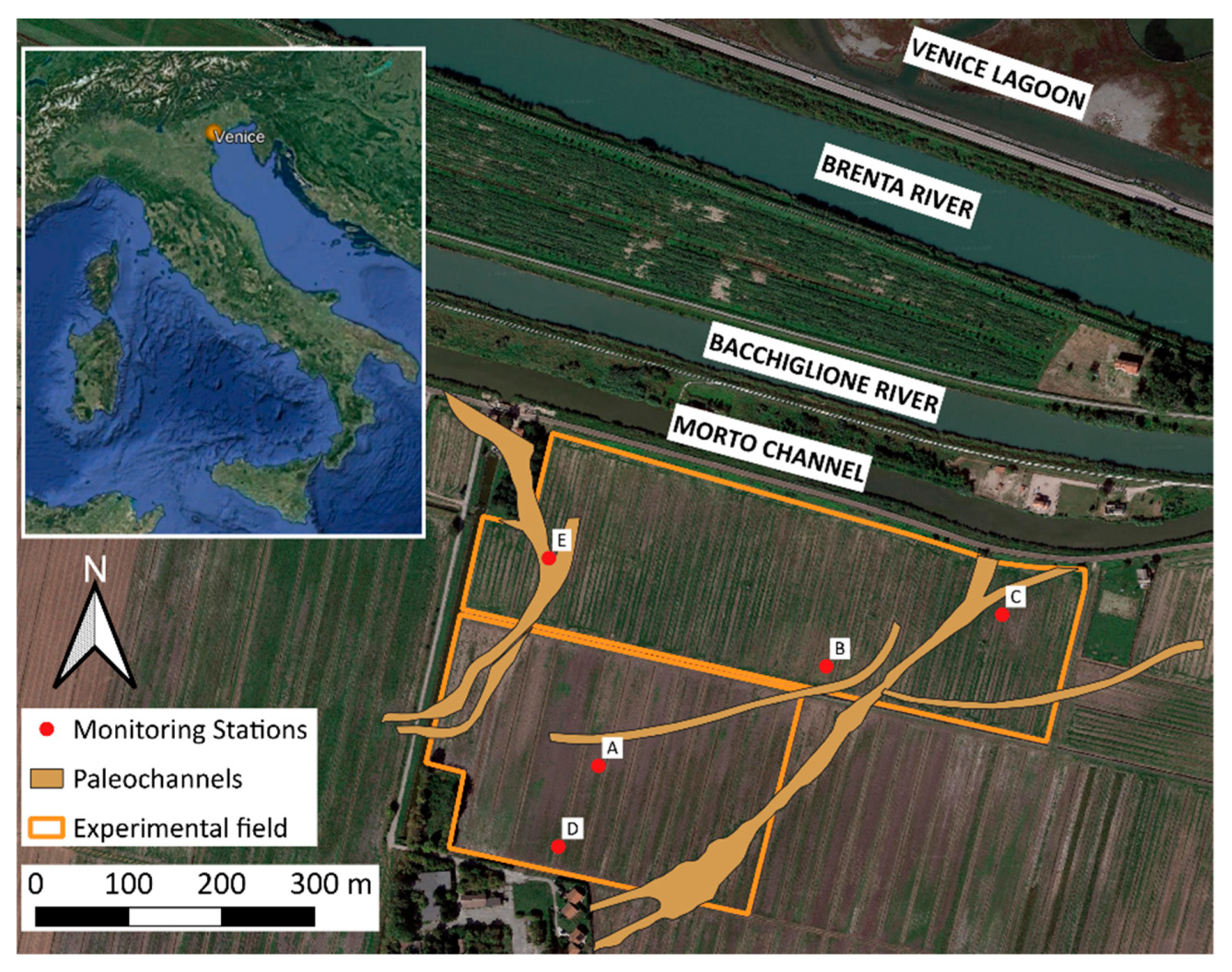
2.1. Experimental Site

The study site is a 21-ha field located at Chioggia, Venice, Italy (45°10′57″ N; 12°13′55″ E) along the southern margin of the Venice Lagoon (Figure 1). It borders the Morto channel, Bacchiglione, and Brenta rivers that flow into the Adriatic Sea 7-km to the west. The field lies below the average sea level, from −1.5 to −3.3 m above mean sea level (msl), and was reclaimed for agricultural purposes between the years 1892 and 1967. The area is affected by saltwater contamination down to about 20 m. The first confined fresh-water aquifer lays at 45–50 m below msl [27].

A pumping station and a dense network of ditches control the depth to the water table, which is generally maintained at 0.6 m below soil surface (bss) during the summer season to promote sub-irrigation. The soil is mainly silt-clay (Molli-Gleyic Cambisol) [28] with the presence of acidic peat [24] and two well-preserved sandy paleochannels crossing the field in a southwest to northeast direction.

The experiment was carried out in the years 2010–2012. The field was cultivated with rainfed maize in 2010 (seeding 22 April, harvest 10 September), 2011 (seeding 4 April, harvest 2 September), and 2012 (seeding 21 March, harvest 11 September). Meteorological data were recorded by an automatic station located 3 km from the experimental site (Regional Agency for Environmental Protection, Veneto).

2.2. Soil and Water Sampling, Analysis, and Monitoring Network

Five monitoring stations (A, B, C, D, and E) were established (Figure 1) in five soil spatial clusters delineated based on the spatial variability of the on-the-go apparent soil electrical conductivity and bare-soil reflectance [29]. Stations A, B, and C were installed in August 2010, while D and E were installed in May 2011 (

Table 1. Soil and water monitoring periods during 2010, 2011, and 2012 at the five monitoring stations.

	2010	2011	2012
A	28 July–15 October 21 December–31 December	1 January–21 March 16 May–23 September	26 April–26 October
B	28 July–15 October 21 December–31 December	1 January–21 March 16 May–23 September	26 April–31 October
C	28 July–15 October 21 December–31 December	1 January–21 March 16 May–23 September	26 April–26 October
D	-	16 May–23 September	26 April–25 October
E	-	16 May–23 September	26 April–26 October

). Monitoring station position and elevation were measured using a Trimble FM 1000 CNH GPS receiver with real-time kinematic (RTK) differential correction (Trimble Navigation Ltd., Sunnyvale, CA, USA). Each station was equipped with: four 5TE (METER Group Inc., Pullman, WA, USA) soil moisture, temperature, and apparent electrical conductivity sensors installed at 0.1, 0.3, 0.5, and 0.7 m of depth connected to an EM50 datalogger (METER Group Inc.); four T8 tensiometers installed at 0.1, 0.3, 0.5, and 0.7 m depths connected to a DL6-TE datalogger (METER Group Inc.); four SK20 micro-lysimeters installed at 0.1, 0.3, 0.5, and 0.7 m depths (METER Group Inc.) to collect soil water samples; one piezometer 2-m deep to measure water table depth, groundwater electrical conductivity (ECw), and collect groundwater samples. Preparation and installation of micro-lysimeters were carried out in accordance with [30].

Soil potential and moisture data were recorded hourly. Soil and groundwater samples were collected manually with an average interval of two weeks. Lysimeter suction was adjusted manually according to the matric potential observations [31]. Sampling frequency was reduced during cultivation operations and very dry conditions, as shown in Table 1. Water samples were stored at 4 °C prior to chemical analysis. Samples were analyzed for electrical conductivity (EC, dS m⁻¹) and pH (SevenMulti pH/conductivity meter, Mettler Toledo, Greifensee, Switzerland), and ionic concentrations (Cl⁻, Br⁻, Na⁺, SO₄²⁻, Mg²⁺, Ca²⁺, K⁺; mg L⁻¹) [32]. All the analyses refer to a standard temperature of 25 °C. Cl/Br, Na/Cl, Mg/Ca, and SO₄/Cl molar ratios were calculated for each water sample.

At the beginning of the experiment, disturbed soil samples were collected at the five monitoring stations at three layers: 0–0.15 m, 0.15–0.45 m, 0.45–0.8 m and analyzed for texture (Mastersizer 2000, Malvern Instruments Ltd., Great Malvern, UK), pH and EC1:2 (1:2 soil–water extract; SevenMulti pH/conductivity meter, Mettler Toledo, Greifensee, Switzerland), total carbon, organic carbon (SOC), total nitrogen, and total sulfur (CNS Vario Macro elemental analyzer, Elementar, Hanau, Germany) [33]. In addition, soil samples were analyzed for exchangeable cations (Mg²⁺, K⁺, Na⁺, and Ca²⁺), cation exchange capacity (CEC), and anion exchange capacity (AEC) [34].

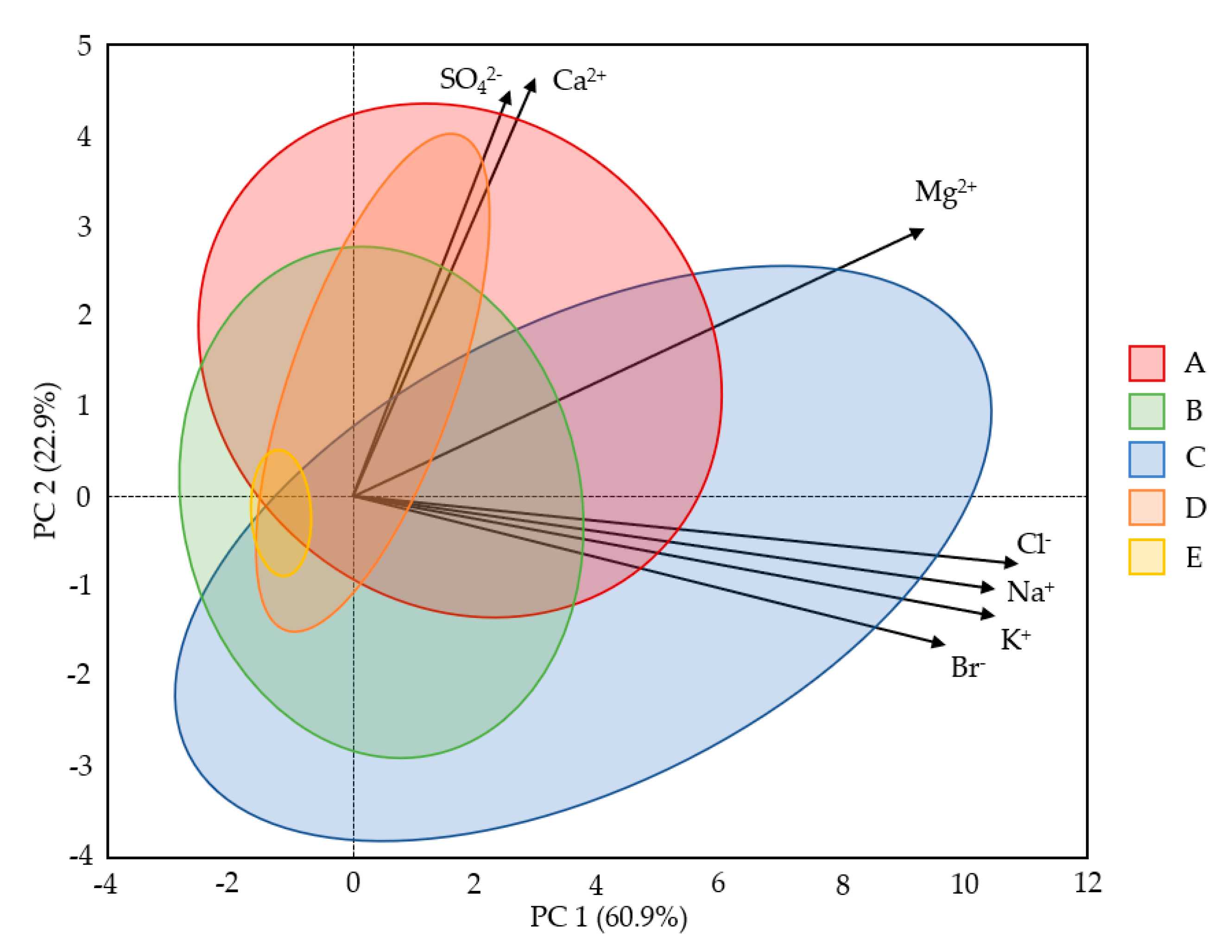
2.3. Statistical Analysis

The interaction between soil water, groundwater, and saltwater was investigated with multivariate statistical techniques. Data were also analyzed according to the water flux direction, which was estimated according to the average daily water potential gradient within the soil profile [35].

The datasets were tested for normality. Since both soil and water data showed a non-normal distribution, statistical analysis was performed with non-parametric methods. Univariate simple statistics was applied to each chemical parameter (i.e., ECw and ionic concentrations). Soil (SOC, pH, EC1:2, texture, carbon and nitrogen content, exchangeable cations) and water chemical parameters (pH, ECw, ion concentrations) were plotted against each other to investigate possible relationships using Spearman’s rank correlation coefficients [36]. Moreover, the principal component analysis (PCA) was performed to determine the correlation structure between the aforementioned variables.

Significant differences in groundwater and soil water ion concentrations and ECw among the five monitoring stations were investigated using the Kruskal Wallis non-parametric test. Post-hoc pair-wise comparisons were performed using the Bonferroni correction to adjust for multiple comparisons. The Kruskal-Wallis test was also applied to investigate significant differences in soil water ion concentrations during upward or downward water fluxes [36].

3. Results

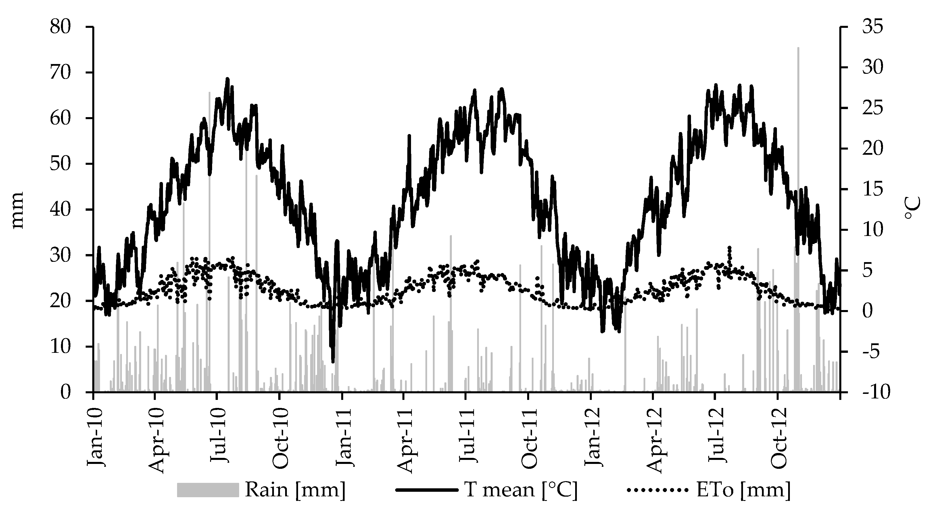
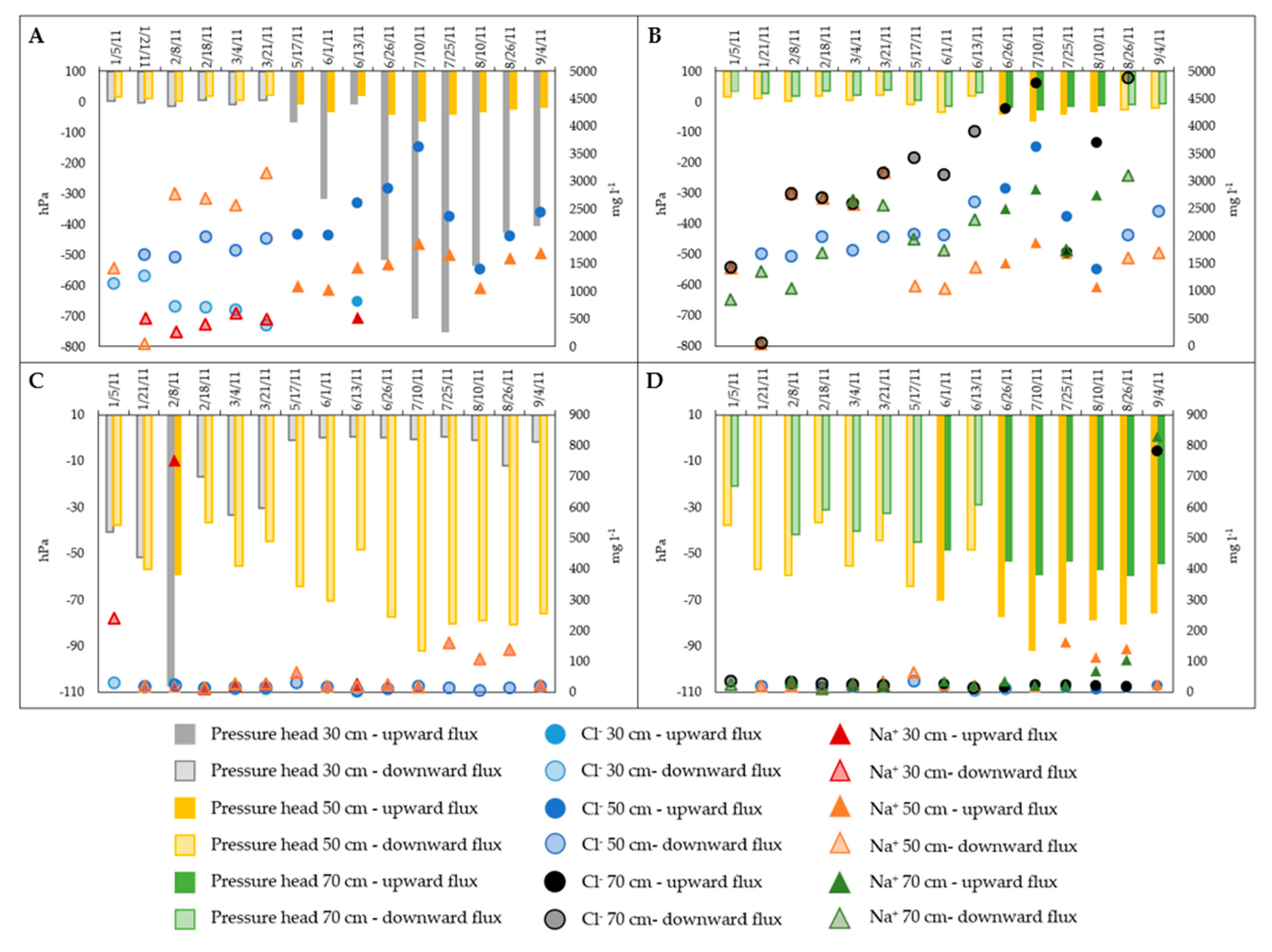
3.1. Weather and Water Table Depth Monitoring

Rainfall and evaporative demand (reference evapotranspiration, ET₀) during the three-year study were higher in 2010 (1116 and 950 mm) than 2011 (506 and 911 mm) and 2012 (720 and 886 mm) (Figure 2). The average depth to the water table ranged from 0.53 m bss at station C to 1.43 m bss at station E, with intermediate levels at stations A (0.73 m bss), B (0.82 m bss), and D (1.14 m bss). The water table elevation (m above the msl) was lower at the innermost station D, from −3.72 to −4.11 m, and higher at station C, close to the Lagoon, ranging from −2.73 to −2.84 m (

Table 2. Minimum, maximum, and average value of depth to the water table [m] below the land surface and above the average sea level.

		A	B	C	D	E
Depth (m below soil surface)	Max	0.94	1.29	0.67	1.04	1.50
	Min	0.56	0.96	0.46	0.65	1.17
	Average	0.74	1.14	0.53	0.82	1.43
Elevation (m above msl)	Max	−3.97	−3.21	−2.73	−3.72	−3.05
	Min	−3.59	−3.54	−2.94	−4.11	−3.38
	Average	−3.77	−3.39	−2.80	−3.89	−3.31

).

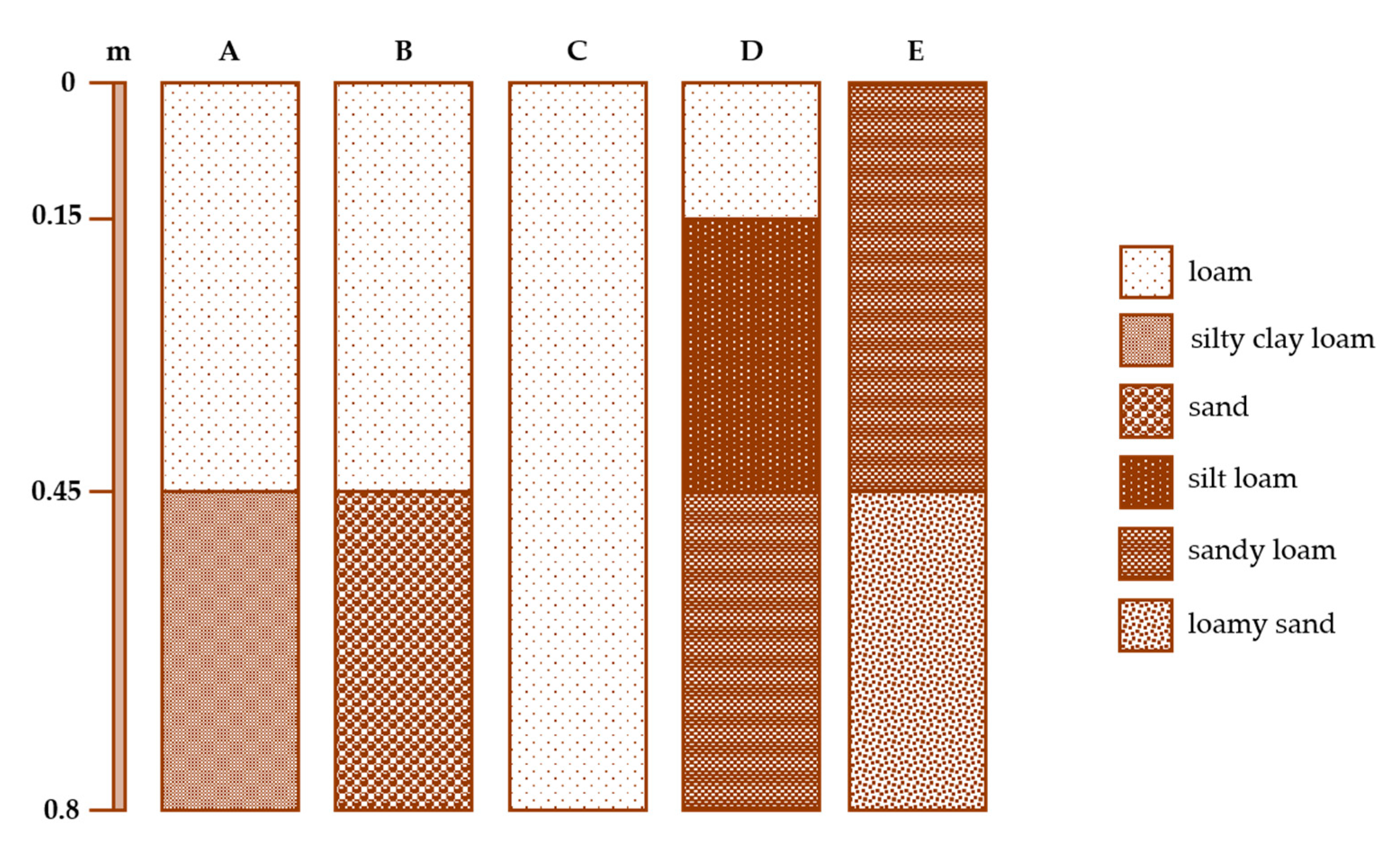
3.2. Soil Characterization

Soil characteristics showed high variability among the five monitoring stations. The top 0.45-m soil layer was mainly loam at station A, B, C, and D, while was sandy at station E, inside the easternmost paleochannel (Figure 1). The deeper 0.45–0.8 m layer was characterized by higher sand content at all the stations except for station A (Figure 3).

Soil pH varied from strongly acidic at station A (<5.5) to alkaline (>7.9) at station E, primarily driven by total carbonates and soil organic carbon (SOC) contents. Total carbonates were 11.39 meq 100 g⁻¹ on average, with minimum and maximum values of 0.5 and 30.0 meq 100 g⁻¹, respectively. Higher contents were observed at the sandier layers of stations B and E. SOC content was 11.6% on average, with peaks >20% due to the presence of acidic peats, particularly at stations A and D. SOC affected also the bulk density (BD), which ranged from 0.21 to 0.94 g cm⁻³ in the organic layers, and electrical conductivity (EC1:2), which peaked to 4.82 ds m⁻¹ at the deeper layer of station C. In mineral layers, BD ranged from 1.37 to 1.52 g cm⁻³ and EC from 0.18 to 1.13 m ds m⁻¹, with lower values observed at the sandy layers of stations B and E. Exchangeable Mg²⁺, Na⁺, Ca²⁺, and K⁺ content was on average 3.13, 1.31, 11.47 and 0.19 meq 100 g⁻¹, respectively. The highest exchangeable cations content was measured at station C and D where the average sum was 20.99 and 22.25 meq 100 g⁻¹, respectively (

Table 3. Soil texture (weight percentage; sand > 50 µm, silt 50–2 µm, clay < 2 µm), pH1:2 (i.e., measured on a 1:2 soil water extract), electrical conductivity (EC1:2, dS m⁻¹), soil organic carbon (SOC, weight percentage, measured on air dried samples), cation-exchange capacity (CEC, meq 100 g⁻¹), carbonates (CaCO₃₋, meq 100 g⁻¹), exchangeable cations (Mg²⁺, Na⁺, Ca²⁺, K⁺, meq 100 g⁻¹), and bulk density (BD, g cm⁻³) that resulted from soil samples collected at 3 depths (0–0.15, 0.15–0.45, and 0.45–0.80 m) per each monitoring station.

Station *	Depth	Sand	Silt	Clay	pH1:2	EC1:2	SOC	CEC	CaCO3	Mg2+	Na+	Ca2+	K+	BD
	m	%				dS m−1	%	meq 100 g−1						g cm−3
A	0–0.15	39.58	40.97	19.45	5.66	0.21	13.72	5.34	11.5	4.72	0.22	11.65	0.21	0.94
A	0.15–0.45	42.27	41.65	16.08	5.54	0.38	15.84	30.56	0.50	4.82	0.30	12.23	0.26	0.77
A	0.45–0.80	17.78	54.57	27.66	5.38	1.13	4.79	15.16	1.00	4.10	0.39	8.74	0.25	1.09
B	0–0.15	51.86	37.21	10.94	7.25	0.35	5.61	12.21	7.08	2.52	0.16	10.64	0.18	1.09
B	0.15–0.45	49.22	38.01	12.76	7.22	0.28	5.96	21.04	7.17	2.57	0.16	10.17	0.18	1.01
B	0.45–0.80	92.09	7.06	0.85	7.70	0.29	2.73	2.35	16.25	1.39	0.15	8.54	0.09	1.2
C	0–0.15	26.87	47.74	25.4	7.67	0.55	8.75	13.95	12.5	2.68	0.84	15.00	0.26	0.94
C	0.15–0.45	32.35	49.18	18.47	7.50	0.88	7.97	16.86	12.25	2.59	0.81	15.04	0.28	0.89
C	0.45–0.80	45.04	39.69	15.27	6.49	4.82	16.34	0.41	7.17	4.31	3.26	17.57	0.33	0.21
D	0–0.15	39.28	47.64	13.09	6.3	0.79	20.81	20.97	-	5.71	0.28	14.29	0.18	0.63
D	0.15–0.45	27.06	50.69	22.25	5.82	0.41	20.41	21.97	0.79	6.10	12.51	14.35	0.28	0.6
D	0.45–0.80	55.95	32.98	11.06	5.62	2.01	21.64	24.4	3.00	3.57	0.28	9.10	0.11	1.01
E	0–0.15	64.66	23.47	11.88	7.39	0.29	1.29	3.23	25.61	0.63	0.06	8.73	0.08	1.52
E	0.15–0.45	61.14	26.69	12.17	7.79	0.2	1.41	3.76	25.31	0.70	0.11	7.98	0.08	1.51
E	0.45–0.80	82.47	12.45	5.08	8.11	0.18	26.99	2.19	29.33	0.54	0.09	7.97	0.05	1.37

* depth to the water table (m below the soil surface) was −0.71 at station A, −1.08 at station B, −0.58 at station C, −1.00 at station D, and −1.47 at station E.

). Average anion exchange capacity (AEC) was 1.28 meq 100 g⁻¹ at station A, 0.8 meq 100 g⁻¹ at station B, 1.96 meq 100 g⁻¹ at station C, 1.86 meq 100 g⁻¹ at station D, and 1.23 meq 100 g⁻¹ at station E.

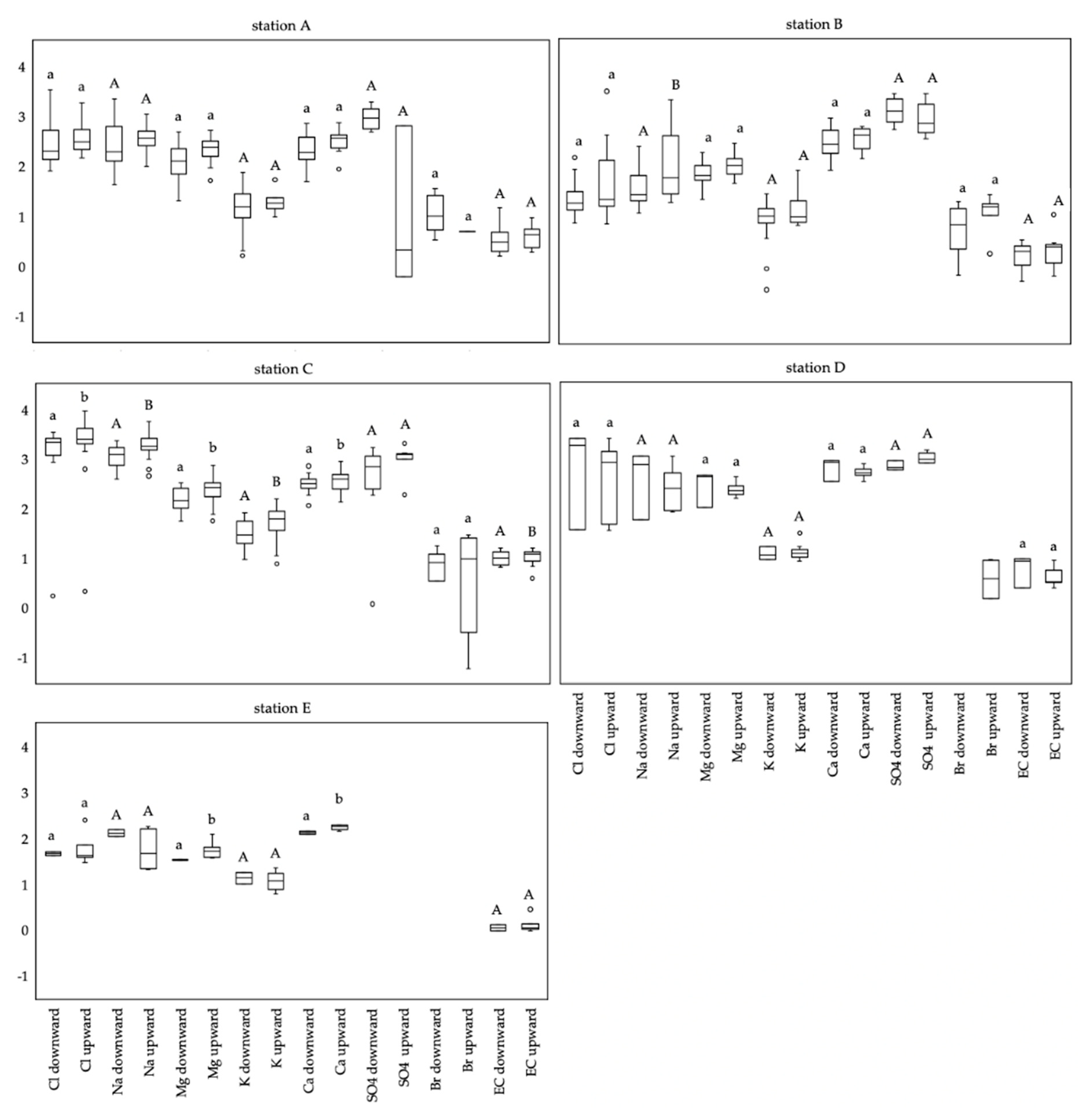
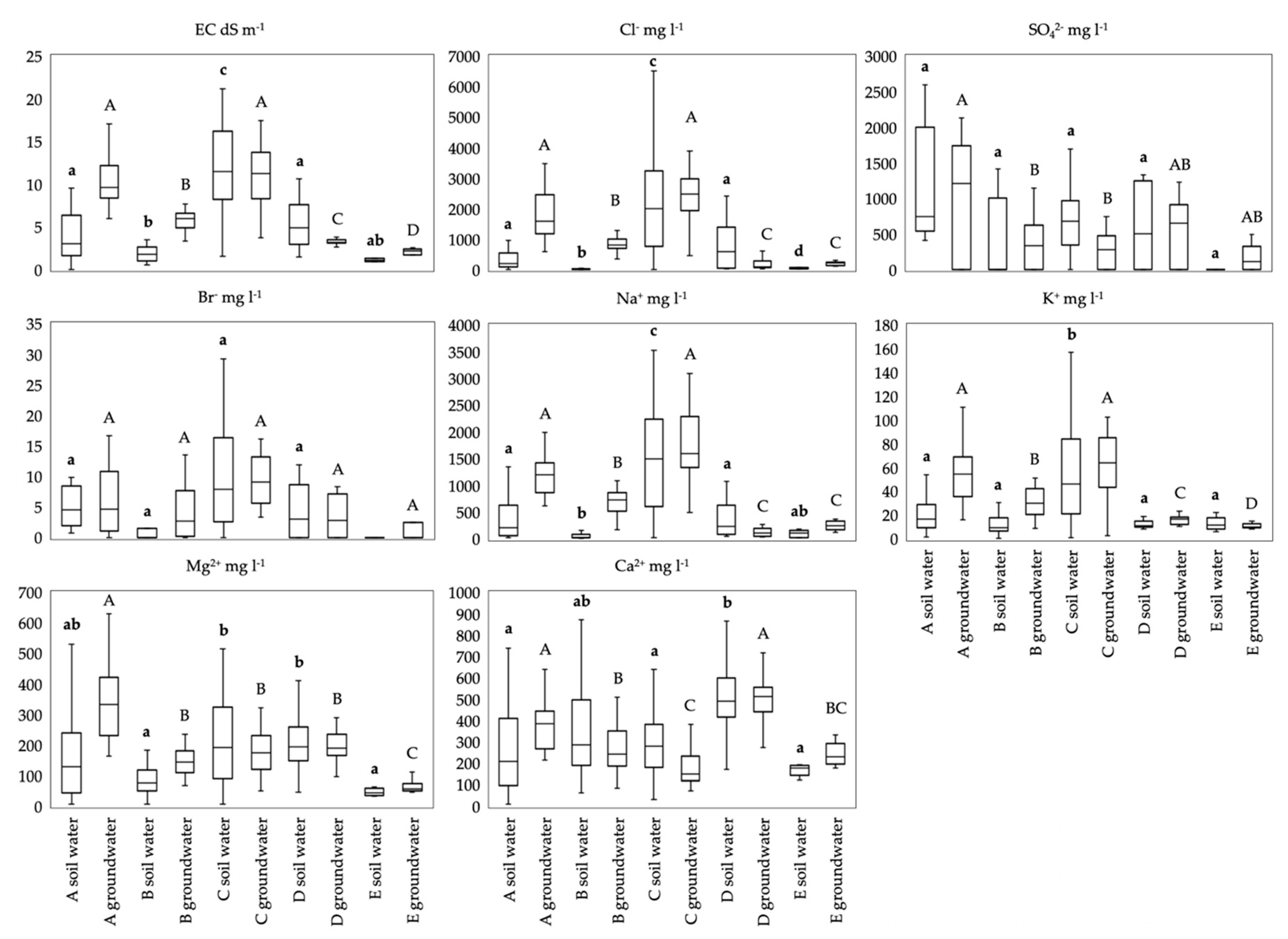
3.3. Soil Water and Groundwater Chemistry

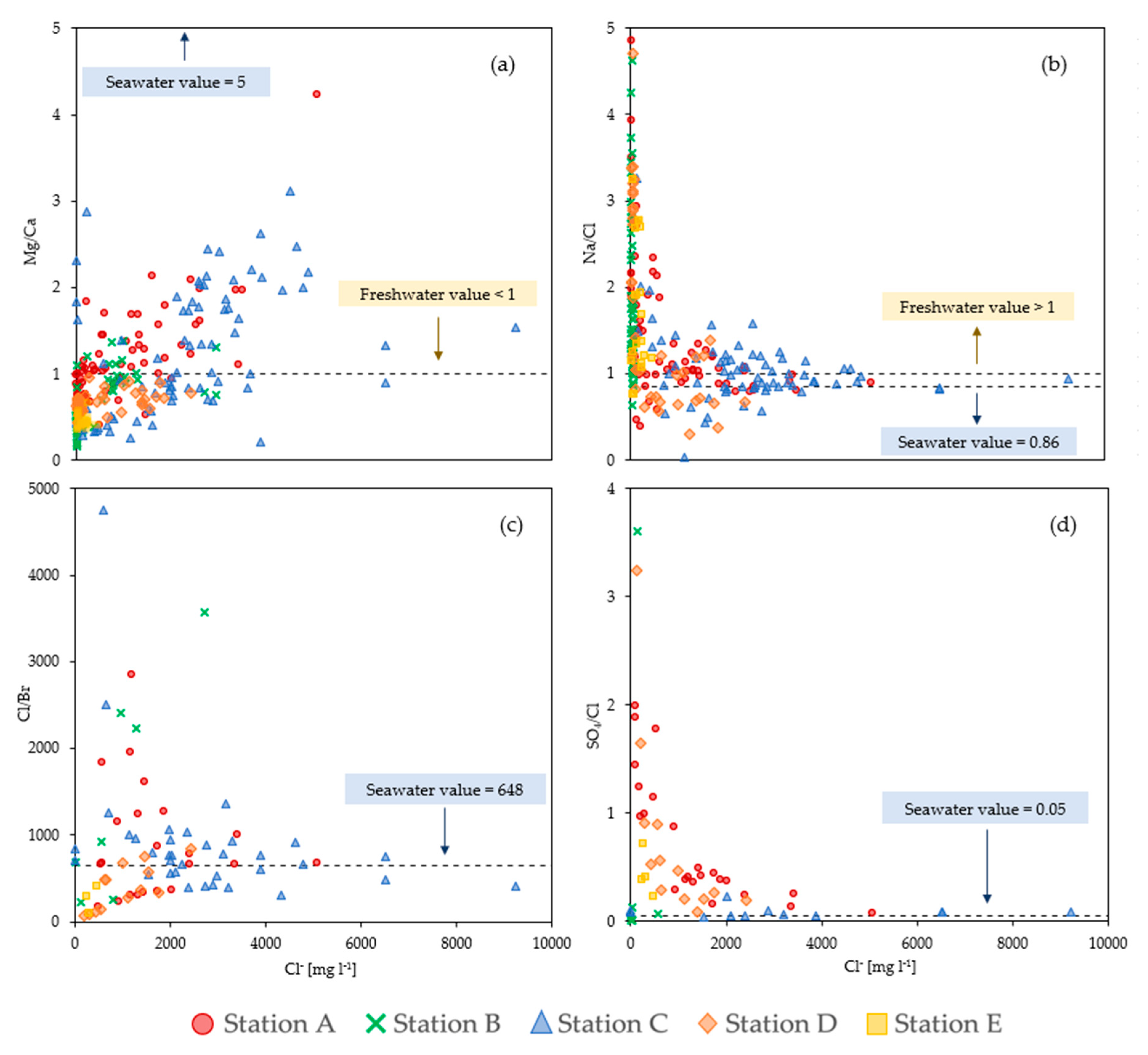
EC and ion concentrations showed high variability across the area, between the sampling depths and dates. In particular, EC ranged from 0.33 to 29.9 dS m⁻¹ with high values observed in the soil and groundwater of station C, the closest to the Lagoon, and low values at the sandier stations B and E (Figure 4). An intermediate situation was observed at stations A and D. Groundwater EC at station D was characterized by small variations during the study period, ranging from 6.86 to 8.04 dS m⁻¹. Groundwater medians were always higher than those found in soil water, even if high peaks were observed in soil water at stations B, C, D, and E.

Cl⁻ and Na⁺ were the most abundant ionic species ranging from 5.74 mg L⁻¹ to 9227.32 mg L⁻¹ and 9.61 mg L⁻¹ to 5624.57 mg L⁻¹, respectively. Concentrations of Br⁻, SO₄²⁻, Mg²⁺, Ca²⁺, and K⁺ varied from 0.7 to 29.29 mg L⁻¹, 0.61 to 2601.97 mg L⁻¹, 6.94 to 630.03 mg L⁻¹, 11.6 to 876.88 mg L⁻¹, and 0.36 to 157.16 mg L⁻¹, respectively (Figure 4). Positive correlations were found between EC, Na⁺, Cl⁻, and K⁺ (p < 0.0001), which were stronger in groundwater than in soil water (e.g., Cl⁻ vs. EC yielded Spearman ρ of 0.92 for groundwater and 0.81 for soil water data). In contrast, correlations between Mg²⁺, Br⁻, and EC were stronger in soil water (e.g., Spearman ρ of Br⁻ vs. EC was 0.46 for groundwater and 0.75 for soil water). Poor dependency was observed when Ca²⁺ and SO₄²⁻ were plotted against EC and the other ions, except for Ca²⁺ vs. Mg²⁺ (

Table 4. Spearman’s correlations between electrical conductivity (EC) and ion concentrations in soil water (white cells) and groundwater (grey cells). Values range from −1 to +1 with larger absolute values indicating a stronger relationship. Bold values indicate significant correlations (α = 0.05).

	ECw	Cl−	Na+	SO42−	Mg2+	Ca2+	K+	Br−
ECw	1.00	0.92	0.91	0.33	0.60	−0.20	0.80	0.46
Cl−	0.81	1.00	0.97	0.18	0.50	−0.19	0.81	0.56
Na+	0.84	0.86	1.00	0.02	0.52	−0.31	0.93	0.58
SO4−	0.38	0.34	0.24	1.00	0.56	0.52	−0.06	−0.03
Mg2+	0.72	0.65	0.74	0.55	1.00	0.46	0.65	0.36
Ca2+	0.42	0.32	0.28	0.59	0.71	1.00	−0.13	−0.15
K+	0.59	0.66	0.80	0.10	0.64	0.18	1.00	0.60
Br−	0.75	0.80	0.81	−0.20	0.61	0.22	0.72	1.00

).

The direction of water flux (i.e., upward or downward water movement) dominated the ion concentration (Figure 5). Station A showed a large variability on Cl⁻, Na⁺, K⁺, SO₄²⁻, Br⁻, and EC during downward flux but higher medians in the upward flux. For instance, 312, 369 mg L⁻¹ and 4.3 dS m⁻¹ vs. 198, 196 mg L⁻¹, and 3.1 dS m⁻¹, respectively for Cl⁻, Na⁺, and EC. Stations B, C, and E confirmed the higher concentrations in the upward movement except for Ca²⁺ (Station C), SO₄²⁻ (station B), and K⁺ (Station E). Station E also differed for the smaller variability in downward flux. Only at station D was Cl⁻, Na⁺, Mg²⁺, and Ca²⁺, and EC higher during the downward movement but with a variability similar to the upward flux. An example of pressure heads vs. Cl⁻ and Na⁺ concentrations observed at different stations, depths, dates, and flux directions is shown in Figure 6.

Post-hoc analysis revealed that Cl⁻ and Na⁺ data found in soil water discriminate between stations A, B, and C (p < 0.005), while groundwater data of stations A and C were not significantly different (Figure 3). The flux direction affected EC and ion concentrations at station C (EC, p = 0.004; Cl⁻, p = 0.022; Na⁺, p = 0.005; Mg²⁺, p = 0.013; K⁺, p = 0.006; Ca⁺; p = 0.018), B (Na⁺, p = 0.031), and E (Mg²⁺, Ca²⁺, p = 0.04) while no differences were found between upward and downward water movement at stations A and D (Figure 5). Br⁻ and SO₄²⁻ demonstrated a conservative behavior, as they were poorly affected by the position (Figure 4) and by the flux direction (Figure 5): Br⁻ did not discriminate between the stations, while SO₄²⁻ discriminate only between groundwater data of stations A, B, and C (p < 0.005).

Significant relationships were found between soil (pH, EC, texture, carbon and nitrogen content, and exchangeable cations) and water characteristics. Soil EC1:2 was positively correlated with water EC (p < 0.0001) and the majority of ions, Cl⁻ (p < 0.0001), Mg²⁺ (p < 0.0001), Na⁺ (p = 0.0001), Br⁻ (p = 0.011) and Ca²⁺ (p = 0.017), with Spearman’s correlation coefficients of 0.89, 0.87, 0.84, 0.81, 0.78, and 0.59, respectively. Moreover, a strong correlation was found between soil exchangeable Na⁺ and water Na⁺ (p = 0.003), Cl⁻ (p = 0.019), K⁺ (p = 0.048), and EC (p = 0.039) with ρ equal to 0.7, 0.58, 0.52, and 0.5, respectively (

Table 5. Spearman’s correlations between soil and soil water chemical properties. Values range from −1 to +1 with larger absolute values indicating a stronger relationship. Bold values indicate significant correlations (α = 0.05).

		Soil Water
		Na+	Mg2+	K+	Ca2+	Cl−	SO42−	Br−	ECw	pH
Soil	Na+	0.70	0.47	0.50	0.06	0.58	0.31	0.14	0.52	−0.19
	Mg2+	0.30	0.26	−0.04	−0.02	0.21	0.28	0.38	0.13	−0.63
	K+	0.59	0.26	0.58	−0.13	0.47	0.28	0.11	0.36	−0.12
	Ca2+	0.52	0.13	0.49	−0.18	0.43	0.04	0.35	0.23	0.11
	CaCO3	−0.14	−0.21	−0.01	−0.04	−0.17	−0.42	−0.18	−0.12	0.61
	EC1:2	0.81	0.84	0.36	0.59	0.87	0.18	0.78	0.89	−0.18
	pH	−0.28	−0.30	−0.08	−0.14	−0.26	−0.45	−0.13	−0.23	0.79

). Soil pH was positively related to water pH (ρ = 0.79, p = 0.0003) but not with water ions.

Principal component analysis (PCA) based on the correlation matrix was carried out for all water samples collected during the three-year study. Most (84%) of the total variability was explained by two principal components. Component 1 (PC 1) was the linear combination of Na⁺, Cl⁻, K⁺, Mg²⁺, and Br⁻ standardized variables and accounted for 60.9% of the variation in the dataset. Component 2 (PC 2) was the linear combination of SO₄²⁻ and Ca²⁺ and accounted for 22.9% of the total variability (Figure 5). Despite the fact that all station ellipses partially overlapped, the effect of the components on station A, C, and D was evident. Station C, the closest to the lagoon, was represented by PC 1, while PC2 was determined by the variability of stations A and D, both located in the southern part of the study site. The sandiest stations B and E seemed not to be strongly discriminated between by the two components (Figure 7).

3.4. Ionic Ratios

Mg/Ca, Na/Cl, Cl/Br, and SO₄/Cl molar ratios were calculated for both soil water and groundwater and plotted with Cl⁻ concentrations (Figure 8). Mg/Ca molar ratio typical of freshwater-seawater mixing (i.e., values ranging between 1 and 5) resulted from samples collected at stations A and C, with values increasing with the Cl⁻ concentration. The vast majority of samples collected at station B, D, and E were characterized by a Mg/Ca ratio close to or lower than 1. In some cases, chloride values typical of seawater intrusion were associated with a Mg/Ca ratio < 1 (e.g., Cl⁻ equal to 3621 mg L⁻¹ and a Mg/Ca ratio of 0.85 observed at station C). The same situation occurred for the Na/Cl ratio, with station A and station C yielding values typical of freshwater-seawater mixing (i.e., values ranging between 0.86 and 1) despite some cases showing Na/Cl ratio values typical of freshwater (>1) but high chloride content. Station D showed Na/Cl ratio values lower than the seawater ratio (<0.86), meaning that there was an excess of Cl⁻ over Na⁺ ion. The Cl/Br ratio was highly variable ranging from a minimum of 66 recorded in groundwater of station D to a maximum of 4746 recorded in soil water of station C. Median values close to seawater ratio were found in groundwater sampled at station A and C (i.e., 684 and 664) and were lower at station B (571 and 576), respectively. Groundwater samples from station D and E were characterized by a lower Cl/Br ratio that corresponded to low Cl⁻ concentrations (i.e., Cl/Br ratio median values of 118 and 289, respectively). The SO₄/Cl molar ratio was almost constant at station C with values equal or lower than the seawater ratio (i.e., 0.05), particularly in groundwater and soil water samples collected at 0.7 m bss (values ranging between 0.036 and 0.057), while a slight increase in the ratio was observed in the shallowest layers with values from 0.081 and 0.099 at 0.5 and 0.3 m bss. The water samples collected at stations A, B, D, and E yielded SO₄/Cl ratios higher than the seawater value.

4. Discussion

Many studies focused on understanding the hydrogeological setting of the coastland at the southern Venice Lagoon. References [9,37] analyzed the exchanges between lagoon water and groundwater using airborne electromagnetic and marine continuous electrical resistivity tomography surveys. More recently, [38] characterized the long-term evolution of groundwater piezometric levels in coastal confined aquifers of Venice, while the origin, extent, and dynamics of the salt contamination, and their relation with the natural and anthropogenic forcing factors was deepened by [7]. However, none of these studies focused on the unsaturated zone and on the hydrogeochemical dynamics involved in seawater-soil water-groundwater exchange interactions.

The research demonstrated that soil water and groundwater were strongly affected by seawater intrusion, with a major effect associated with Cl⁻ and Na⁺ concentration (Figure 4). Two different chemical components were identified from PCA: a first one formed by Cl⁻, Na⁺, Br⁻, K⁺, and Mg²⁺ and a second one composed by SO₄²⁻ and Ca²⁺ (Figure 7). The first component varied across the field according to the soil properties and the distance from the coastline, while the second one was more homogenous and did not vary across monitoring stations. This agrees with the results obtained by [18,19] who defined Br⁻ and SO₄²⁻ as conservative tracers, since they were not involved in soil exchange interactions. In contrast, cation exchange reactions due to salinization and freshening processes cause depletion or enrichment of water Na⁺, K⁺, Ca²⁺, and Mg²⁺ [39].

Seawater intrusion-driven water quality was noticeable at station C, the closest to the coastline, characterized by the highest elevation and shallowest water table. The 0.6–0.8 m soil layer was saturated throughout nearly all of all the study period and the water table frequently reached a 0.5 m depth bss. Both soil water and groundwater were characterized by high Cl⁻ and Na⁺ contents and anions Cl⁻ > SO₄²⁻. The majority of 0.7 m and groundwater samples were characterized by Na > Mg > Ca > K that equal the sequence found in seawater [3]. In contrast, water samples collected at the top layers were characterized by the cation sequence Na > Ca > Mg > K with the excess of Ca²⁺ over Mg²⁺, which can be explained by the soil calcareous parent materials [17]. This was confirmed by Mg/Ca ratio values that showed medians lower than seawater ratio (<1) at 0.1, 0.3, and 0.5 m bss, and median values typical of freshwater-seawater mixing at 0.7 m bss and in groundwater (>1) [23]. The SO₄/Cl and Cl/Br ratios also reflected the effect of seawater intrusion in groundwater being about 0.05 and 664, respectively. Moreover, Cl/Br ratio reflected the effect of both freshening processes (e.g., during rain events) that lowered its value (<500), and salinization events (e.g., dry deposition of marine aerosol) that increased its value (>800) [19]. Moreover, the ionic concentration was higher during the upward water movement (Figure 5), demonstrating that soil water salinity mostly originated from the brackish groundwater.

Station B and E were mainly characterized by mineral soil-driven water quality. They were both located in the coarser portion of the paleochannels, in the site-specific management unit III identified by [24] and characterized by high sand percentage, high bulk density, and low SOC. Soil water and groundwater were characterized by low salinity, as a result of the high percolation and low CEC of the sandy soil [24,40]. Ca²⁺ was the most abundant cation in soil water samples, while Na⁺ > Ca²⁺ was found in groundwater samples, meaning that seawater was able to sporadically intrude into groundwater. This was confirmed by the highest Cl⁻, Na⁺, Mg²⁺, and K⁺ concentrations observed during the upward water movement. Low values of the Mg/Ca ratio and high values of the Na/Cl ratio relative to seawater may be caused by high CaCO₃ content in soil (Table 3) and its dissolution [17].

Stations A and D were located in peaty, acidic, and moderately saline areas [24,29]. The pH between 5.4 and 6.3, low carbonates, great organic carbon content, high concentration of dissolved SO₄²⁻, and the tidal origin of the area suggested that those stations were located in a potential acidic sulfate environment where the presence of dissolved SO₄²⁻ was a consequence of oxidation and rewetting of acid sulfate horizons formed under waterlogged conditions and exposed to aerobic conditions after their reclamation [41,42]. The strong relationship between those stations, SO₄²⁻, and Ca²⁺ was demonstrated by the PCA (Figure 7). The soil pedogenesis suggested by SO₄²⁻ observations was also confirmed by the high concentration of soluble salts found in both stations that is typical of tidal and recently reclaimed sulfidic soils subject to prolonged flooding by seawater [41]. Post-hoc statistical analysis revealed that the stations were no different for ion concentrations of soil water, while the major ions characterizing seawater discriminated between the station groundwater (Figure 4). Station A was located in a silty area, soil water salinity was mainly driven by SO₄²⁻ anion, while groundwater salinity was saltier and dominated by Cl⁻. The opposite situation occurred at station D, located in a sandier area, where SO₄²⁻ > Cl⁻ and Ca²⁺ > Na⁺ were observed in groundwater, while Cl⁻ > SO₄²⁻ in soil water. The greater SOC presence at station D and the coarser texture may explain the great presence of SO₄²⁻ and Ca²⁺ in groundwater, while the fine texture observed at station A increased the capacity of soil to retain SO₄²⁻ anions. The excess of Ca²⁺ observed in groundwater of station D was probably caused by the dissolution of CaCO₃ in the soil following acidification [39], while the excess of Na⁺ found in soil (Table 3) could be explained by the presence of peat and by its ability to retain cations [43]. Cl/Br medians of station A were typical of those found in coastal areas affected by seawater intrusion [19], while Cl decreased with soil depth at station D, causing the decrease of Cl/Br medians.

5. Conclusions

The hydrogeochemical processes involved in the seawater intrusion phenomenon were investigated to point out the major threats to groundwater quality and farmland productivity near the Venice Lagoon.

The applicability of ionic ratios as tracers for the identification of saltwater contamination was validated and implemented by studying the origin of both groundwater and soil water salinity. This approach allowed a precise characterization of the study site distinguishing between the degree of contamination of soil and groundwater.

Soil and water chemical characteristics confirmed that the study site was strongly affected by seawater intrusion, although different dynamics were identified. Two main contamination processes were pointed out: salinization directly linked to seawater intrusion and salinization mainly derived by the interaction between peaty soil and salts. In the first case, soil and groundwater were dominated by Cl⁻ and Na⁺ ions and characterized by ionic ratios typical of this process, while the interaction between high SOC and salinity determined an excess of SO₄²⁻ ion in the peaty areas. A different situation occurred in the coarser locations, where the low CEC promoted percolation so that seawater ions were easily leached, and ionic ratios were similar to those found in freshwater.

Results suggested that reclaimed marshes near the Venice Lagoon have the potentiality to become an acidic sulfate environment. Toxicity and deterioration of soil properties associated with seawater intrusion could be worsened by chemical limitations associated with acid sulfate horizons (i.e., aluminum toxicity and nutrient deficiencies). Under these conditions, the range of crops that could be grown would be severely restricted and yield would be drastically reduced.

The adopted methodology could be extended to further characterize the spatial variability of soil salinization in the entire northern Adriatic coast and in other regions with similar characteristics (e.g., coastal low-lying plains). Moreover, this approach would allow to outline best strategies for the management of saltwater contamination depending on the salt origin: the installation of infrastructures preventing salt intrusion from the sea or lagoon to the farmland, rather than strategies promoting leaching and pH correction in the case of processes linked to peat presence. Future research is also needed to investigate the relationship between peaty soils typical of reclaimed areas and seawater intrusion, and to further confirm the possibility that those soil become sulfidic.

References

1. Mondal, N.C.; Singh, V.P.; Singh, V.S.; Saxena, V.K. Determining the interaction between groundwater and saline water through groundwater major ion chemistry. J. Hydrol. Hydrol. 2010, 388, 100–111. [Google Scholar] [CrossRef]
2. Carbognin, L.; Tosi, L. Il Progetto ISES per L’analisi dei Processi di Intrusione Salina e Subsidenza nei Territori Meridionali delle Province di Padova e Venezia; Istituto per lo Studio della Dinamica delle Grandi Masse, Consiglio Nazionale di Ricerca: Venice, Italy, 2003; pp. 16–88. [Google Scholar]
3. Werner, A.D.; Bakker, M.; Post, V.E.A.; Vandenbohede, A.; Lu, C.; Ataie-Ashtiani, B.; Simmons, C.T.; Barry, D.A. Seawater intrusion processes, investigation and management: Recent advances and future challenges. Adv. Water Resour. 2013, 51, 3–26. [Google Scholar] [CrossRef]
4. Brambati, A.; Carbognin, L.; Quaia, T.; Teatini, P.; Tosi, L. The Lagoon of Venice: Geological setting, evolution and land subsidence. Episodes 2003, 26, 264–268. [Google Scholar] [CrossRef] [PubMed]
5. Gambolati, G.; Putti, M.; Teatini, P.; Gasparetto-Stori, G. Subsidence due to peat oxidation and impacts on drainage infrastructures in a farmland catchment south of the Venice Lagoon. Environ. Geol. 2006, 49, 814–820. [Google Scholar] [CrossRef]
6. Carbognin, L.; Teatini, P.; Tosi, L. Land subsidence in the Venetian area: Known and recent aspects. G. Geol. Appl. 2005, 1, 5–11. [Google Scholar]
7. Da Lio, C.; Carol, E.; Kruse, E.; Teatini, P.; Tosi, L. Saltwater contamination in the managed low-lying farmland of the Venice coast, Italy: An assessment of vulnerability. Sci. Total Environ. 2015, 533, 356–369. [Google Scholar] [CrossRef]
8. Mulligan, A.E.; Evans, R.L.; Lizarralde, D. The role of paleochannels in groundwater/seawater exchange. J. Hydrol. 2007, 335, 313–329. [Google Scholar] [CrossRef]
9. De Franco, R.; Biella, G.; Tosi, L.; Teatini, P.; Lozej, A.; Chiozzotto, B.; Giada, M.; Rizzetto, F.; Claude, C.; Mayer, A.; et al. Monitoring the saltwater intrusion by time lapse electrical resistivity tomography: The Chioggia test site (Venice Lagoon, Italy). J. Appl. Geophys. 2009, 69, 117–130. [Google Scholar] [CrossRef]
10. Di Sipio, E.; Galgaro, A.; Zuppi, G.M. New geophysical knowledge of groundwater systems in Venice estuarine environment. Estuar. Coast. Shelf Sci. 2006, 66, 6–12. [Google Scholar] [CrossRef]
11. El Moujabber, M.; Bou Samra, B.; Darwish, T.; Atallah, T. Comparison of Different Indicators for Groundwater Contamination by Seawater Intrusion on the Lebanese Coast. Water Resour. Manag. 2006, 20, 161–180. [Google Scholar] [CrossRef]
12. Millero, F.J.; Feistel, R.; Wright, D.G.; McDougall, T.J. The composition of Standard Seawater and the definition of the Reference-Composition Salinity Scale. Deep-Sea Res. Part I 2008, 55, 50–72. [Google Scholar] [CrossRef]
13. Sukhija, B.S.; Varma, V.N.; Nagabhushanam, P.; Reddy, D.V. Differentiation of paleomarine and modern seawater intruded salinities in coastal groundwaters (of Karaikal and Tanjavur, India) based on inorganic chemistry, organic biomarker fingerprints and radiocarbon dating. J. Hydrol. 1996, 174, 173–201. [Google Scholar] [CrossRef]
14. FAO. Seawater Intrusion in Coastal Aquifers: Guidelines for Studying, Monitoring and Control; Food and Agriculture Organization of the United Nations: Rome, Italy, 1997; pp. 5–23. [Google Scholar]
15. Ghabayen, S.M.S.; McKee, M.; Kemblowski, M. Ionic and isotopic ratios for identification of salinity sources and missing data in the Gaza aquifer. J. Hydrol. 2006, 318, 360–373. [Google Scholar] [CrossRef]
16. Vengosh, A.; Gill, J.; Davisson, M.L.; Hudson, G.B. A multi-isotope (B, Sr, O, H and C) and age dating (3H-3He and 14C) study of groundwater from Salinas Valley, California: Hydrogeochemistry, dynamics, and contamination processes. Water Resour. Res. 2002, 38, 1008. [Google Scholar] [CrossRef]
17. Vengosh, A.; Rosenthal, E. Saline groundwater in Israel: Its bearing on the water crisis in the country. J. Hydrol. 1994, 156, 389–430. [Google Scholar] [CrossRef]
18. Vengosh, A.; Spivack, A.J.; Artzi, Y.; Ayalon, A. Geochemical and boron, strontium, and oxygen isotopic constraints on the origin of the salinity in groundwater from the Mediterranean coast of Israel. Water Resour. Res. 1999, 35, 1877–1894. [Google Scholar] [CrossRef]
19. Alcalá, F.J.; Custodio, E. Using the Cl/Br ratio as a tracer to identify the origin of salinity in aquifers in Spain and Portugal. J. Hydrol. 2008, 359, 189–207. [Google Scholar] [CrossRef]
20. Abrol, I.P.; Yadav, J.S.P.; Massoud, F.I. Salt-Affected Soil and Their Management; FAO Soils Bulletin 39; Food and Agriculture organization of the United Nations: Rome, Italy, 1988. [Google Scholar]
21. Kim, Y.; Lee, K.S.; Koh, D.C.; Lee, D.H.; Lee, S.G.; Park, W.B.; Koh, G.W.; Woo, N.C. Hydrogeochemical and isotopic evidence of groundwater salinization in a coastal aquifer: A case study in Jeju volcanic island, Korea. J. Hydrol. 2003, 270, 282–294. [Google Scholar] [CrossRef]
22. Lee, J.Y.; Song, S.H. Evaluation of groundwater quality in coastal areas: Implications for sustainable agriculture. Environ. Geol. 2007, 52, 1231–1242. [Google Scholar] [CrossRef]
23. Pulido-Leboeuf, P.; Pulido-Bosh, A.; Calvache, M.L.; Vallejos, Á.; Andreu, J.M. Strontium, SO42−/Cl and Mg2+/Ca2+ ratios as tracers for the evolution of seawater into coastal aquifers: The example of Castell de Ferro aquifer (SE Spain). Comptes Rendus Geosci. 2003, 335, 1039–1048. [Google Scholar] [CrossRef]
24. Scudiero, E.; Teatini, P.; Corwin, D.L.; Dal Ferro, N.; Simonetti, G.; Morari, F. Spatiotemporal Response of Maize Yield to Edaphic and Meteorological Conditions in a Saline Farmland. Agron. J. 2014, 106, 2163–2174. [Google Scholar] [CrossRef] [Green Version]
25. Ayers, R.; Westcot, D. Water Quality for Agriculture; FAO Irrigation and Drainage Paper No. 29 Rev.1; Food and Agriculture Organization of the United Nations: Rome, Italy, 1985. [Google Scholar]
26. Volpe, V.; Manzoni, S.; Marani, M.; Katul, G. Leaf conductance and carbon gain under salt-stressed conditions. J. Geophys. Res. 2011, 116, G04035. [Google Scholar] [CrossRef]
27. Viezzoli, A.; Tosi, L.; Teatini, P.; Silvestri, S. Surface water-groundwater exchange in transitional coastal environments by airborne electromagnetics: The Venice Lagoon example. Geophys. Res. Lett. 2010, 37, L01402. [Google Scholar] [CrossRef]
28. FAO-UNESCO. Soil Map of the World, Revised Legend; Food and Agriculture Organization of the United Nations: Rome, Italy, 1989. [Google Scholar]
29. Scudiero, E.; Teatini, P.; Corwin, D.L.; Deiana, R.; Berti, A.; Morari, F. Delineation of site-specific management units in a saline region at the Venice Lagoon margin, Italy, using soil reflectance and apparent electrical conductivity. Comput. Electron. Agric. 2013, 99, 54–64. [Google Scholar] [CrossRef]
30. Morari, F. Drainage Flux Measurement and Errors Associated with Automatic Tension-controlled Suction Plates. Soil Sci. Soc. Am. J. 2006, 6, 1860–1871. [Google Scholar] [CrossRef]
31. Ciglasch, H.; Amelung, S.; Totrakool, S.; Kaupenjohann, M. Water flow patterns and pesticide fluxes in an upland soil in northern Thailand. Eur. J. Soil Sci. 2005, 56, 765–777. [Google Scholar] [CrossRef]
32. APAT; CNR-IRSA. Metodi Analitici per le Acque; APAT: Rome, Italy, 2003. [Google Scholar]
33. Nelson, D.W.; Sommers, L.E. Total Carbon, Organic Carbon and Organic Matter. In Methods of Soil Analysis Part 3: Chemical Methods; Sparks, D.L., Ed.; Soil Science Society of America, American Society of Agronomy: Madison, WI, USA, 1996; pp. 961–1010. [Google Scholar]
34. Sumner, M.E.; Miller, W.P. Cation Exchange Capacity and Exchange Coefficients. In Methods of Soil Analysis Part 3: Chemical Methods; Sparks, D.L., Ed.; Soil Science Society of America, American Society of Agronomy: Madison, WI, USA, 1996; pp. 1201–1230. [Google Scholar]
35. Hillel, D. Introduction to Environmental Soil Physics; Elsevier: San Diego, CA, USA, 2004; p. 494. [Google Scholar]
36. Schabenberger, O.; Pierce, F.J. Contemporary Statistical Models for the Plant and Soil Sciences; CRC Press: Boca Raton, FL, USA, 2001; p. 725. [Google Scholar]
37. Teatini, P.; Tosi, L.; Viezzoli, A.; Bardello, L.; Zecchin, M.; Silvestri, S. Understanding the hydrogeology of the Venice Lagoon subsurface with airborne electromagnetics. J. Hydrol. 2011, 411, 342–354. [Google Scholar] [CrossRef]
38. Da Lio, C.; Tosi, L.; Zambon, G.; Vianello, A.; Baldin, G.; Lorenzetti, G.; Manfè, G.; Teatini, P. Long-term groundwater dynamics in the oastal confined aquifers of Venice (Italy). Estuar. Coast. Shelf Sci. 2013, 135, 248–259. [Google Scholar] [CrossRef]
39. Russak, A.; Sivan, O. Hydrogeochemical Tool to Identify Salinization or Freshening of Coastal Aquifers Determined from Combined Field Work, Experiments, and Modeling. Environ. Sci. Technol. 2010, 44, 4096–4102. [Google Scholar] [CrossRef]
40. Grosso, C.; Manoli, G.; Martello, M.; Chemin, Y.H.; Pons, D.H.; Teatini, P.; Piccoli, I.; Morari, F. Mapping Maize Evapotranspiration at Field Scale Using SEBAL: A Comparison with the FAO Method and Soil-Plant Model Simulations. Remote Sens. 2018, 10, 1452. [Google Scholar] [CrossRef] [Green Version]
41. Dent, D. Acid Sulphate Soils: A Baseline for Research and Development; International Institute for Land Reclamation and Improvement: Wageningen, The Netherlands, 1986; pp. 22–73. [Google Scholar]
42. Mosley, L.M.; Zammit, B.; Jolley, A.; Barnett, L.; Fitzpatrick, R. Monitoring and assessment of surface water acidification following rewetting of oxidised acid sulfate soils. Environ. Monit. Assess. 2014, 186, 1–18. [Google Scholar] [CrossRef] [PubMed]
43. Keesstra, S.D.; Geissen, V.; Mosse, K.; Piiranen, S.; Scudiero, E.; Leistra, M.; van Schaik, L. Soil as a filter for groundwater quality. Curr. Opin. Environ. Sustain. 2012, 4, 507–516. [Google Scholar] [CrossRef]
Figure 1. Map of the study area depicting the paleochannels and the monitoring stations.
Water 12 03363 g001
Figure 2. Rain, temperature, and reference evapotranspiration (ET0) data recorded during 2010, 2011 and 2012.
Water 12 03363 g002
Figure 3. Soil profile (USDA texture classes) found at the monitoring stations (A, B, C, D, E).
Water 12 03363 g003
Figure 4. Box plot of electrical conductivity (EC) and ion concentration in soil water and groundwater of each monitoring station. Letters refer to post-hoc statistical analysis (Wilcoxon test on each pair). Different lowercase letters indicate significant differences between soil water data, while capital letters refer to groundwater data. α was corrected for multiple comparisons using the Bonferroni procedure (α = 0.005).
Water 12 03363 g004
Figure 5. Pressure heads (hPa), Cl and Na+ (mg L−1) concentrations observed at station C and B on different dates. (A) station C, 30–50 cm flux; (B) station C, 50–70 cm flux; (C) station B, 30–50 cm flux; (D) station B, 50–70 cm flux.
Water 12 03363 g005
Figure 6. Box plot of ion concentration distributions (logarithmic scale) during upward and downward water movement for each monitoring station. Outliers are plotted as individual points. Letters refer to post-hoc statistical analysis (Kruskal Wallis test). Different letters indicate significant differences (α = 0.05) between ion and electrical conductivity (EC) movement along the soil profile. Lowercase and capital letters were alternately used to distinguish between each pairwise comparison.
Water 12 03363 g006
Figure 7. Biplot showing the principal component analysis (PCA) score plot overlaid with the loading plot for principal component 1 (PC 1) and principal component 2 (PC 2). Each ellipse shows where 95% of data of each station are expected to lie.
Water 12 03363 g007
Figure 8. Mg/Ca (a), Na/Cl (b), Cl/Br (c), and SO4/Cl (d) molar ratios as function of Cl concentration [mg L−1].
Water 12 03363 g008