An Analysis of Streamflow Trends in the Southern and Southeastern US from 1950–2015


Abstract
1. Introduction
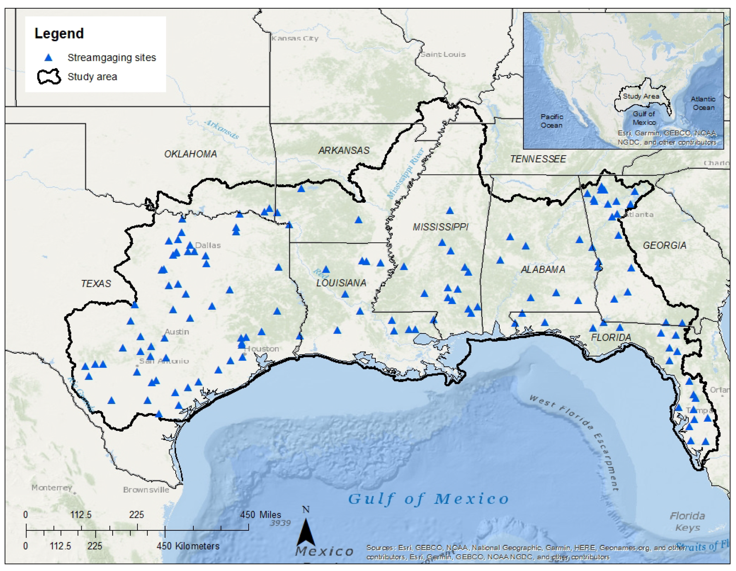
2. Study Area
3. Materials and Methods
3.1. Data Preparation and Site Selection
3.2. Mann–Kendall and Correlation Analysis of Time-Series Data for Clusters of Sites
3.3. Mann–Kendall and Quantile-Kendall Trend Analysis of Time-Series Data at Individual Sites
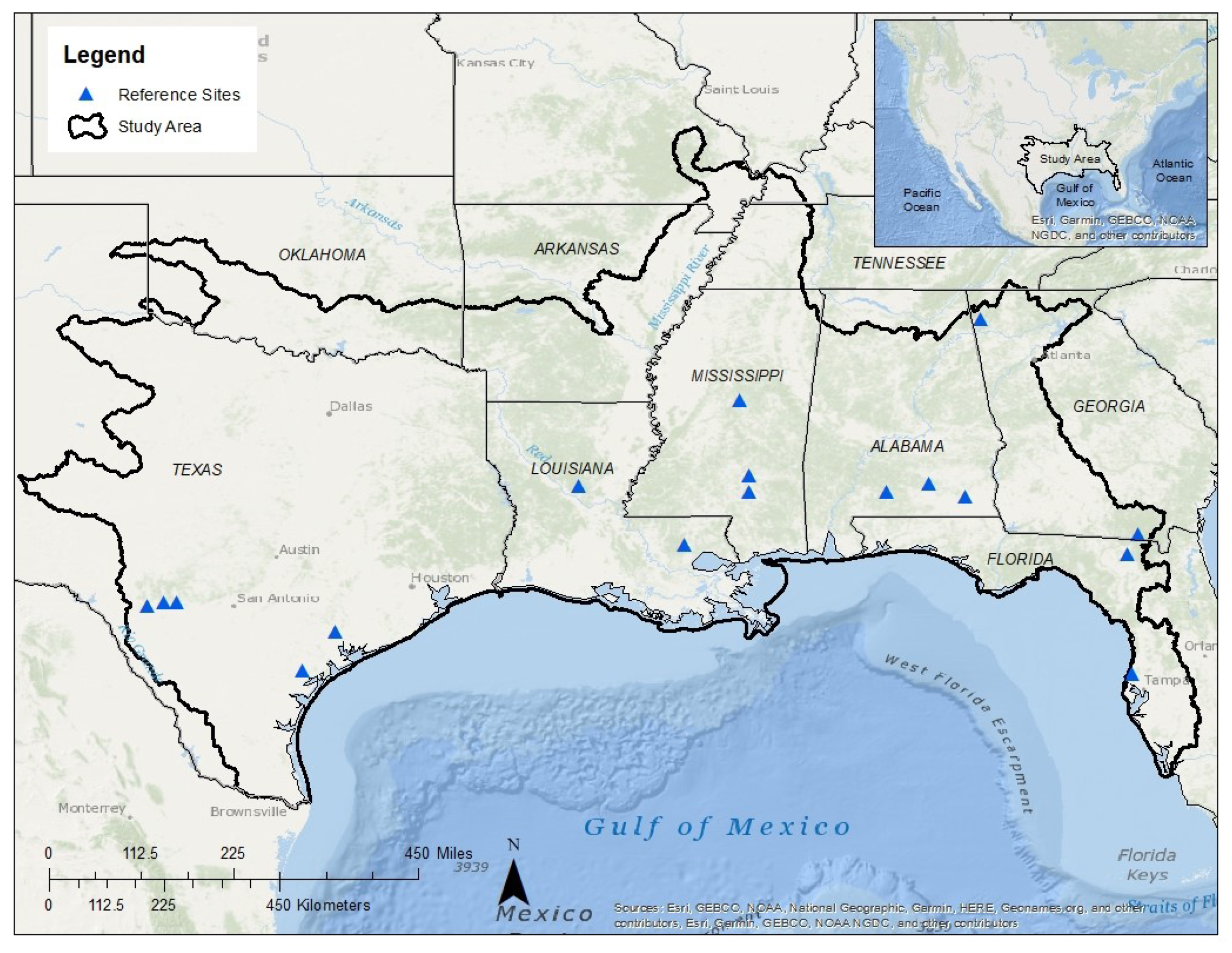
3.4. Comparison of Each Site’s Trend Results to Reference Conditions
4. Results and Discussion
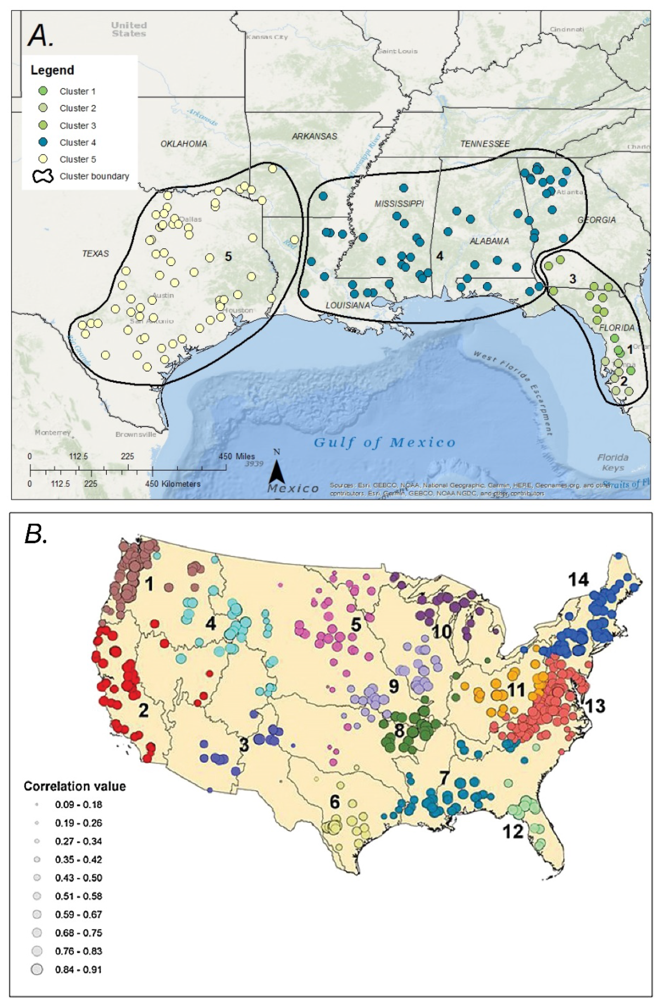
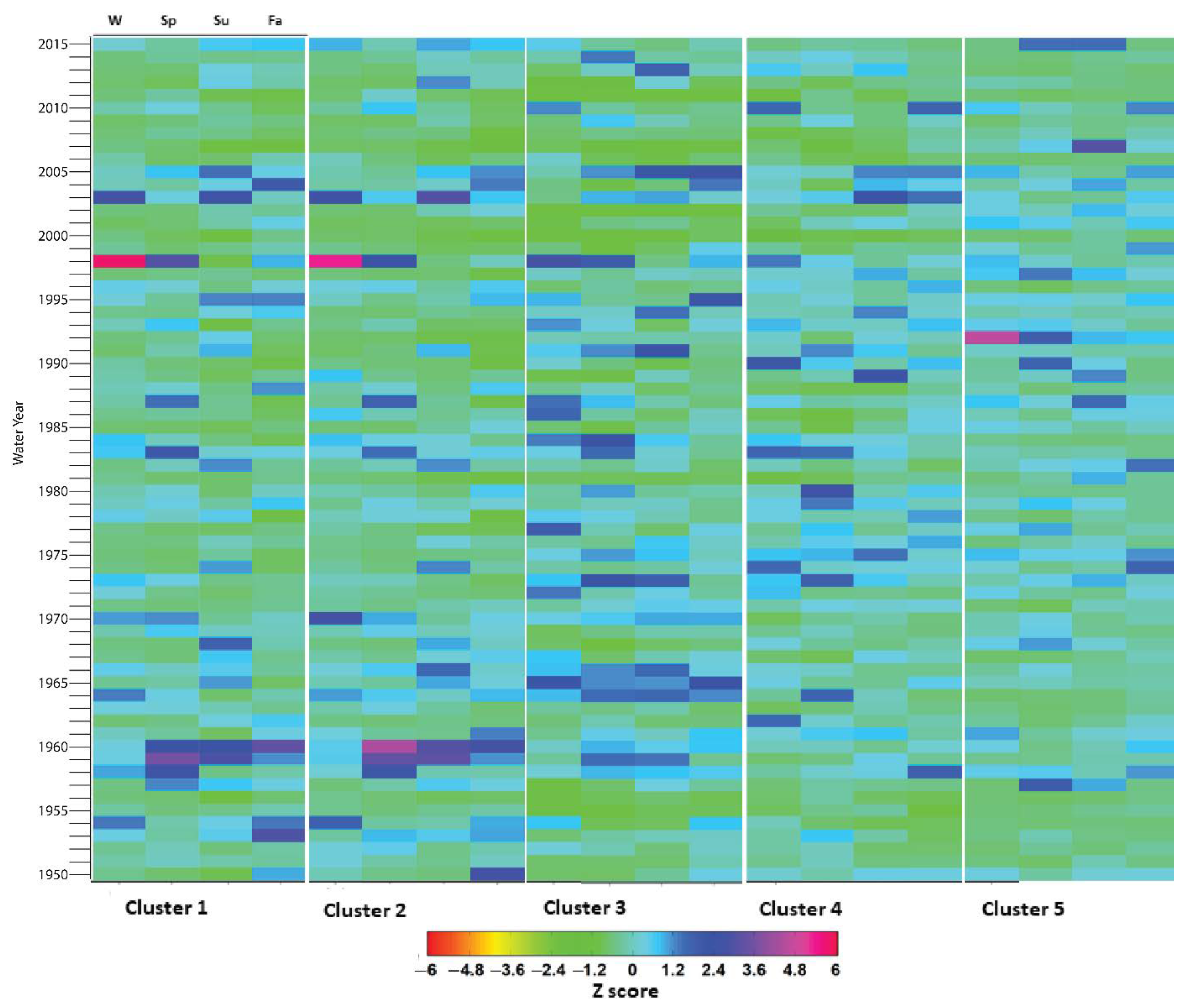
4.1. Cluster Analysis and Trends in Cluster-Mean Time-Series
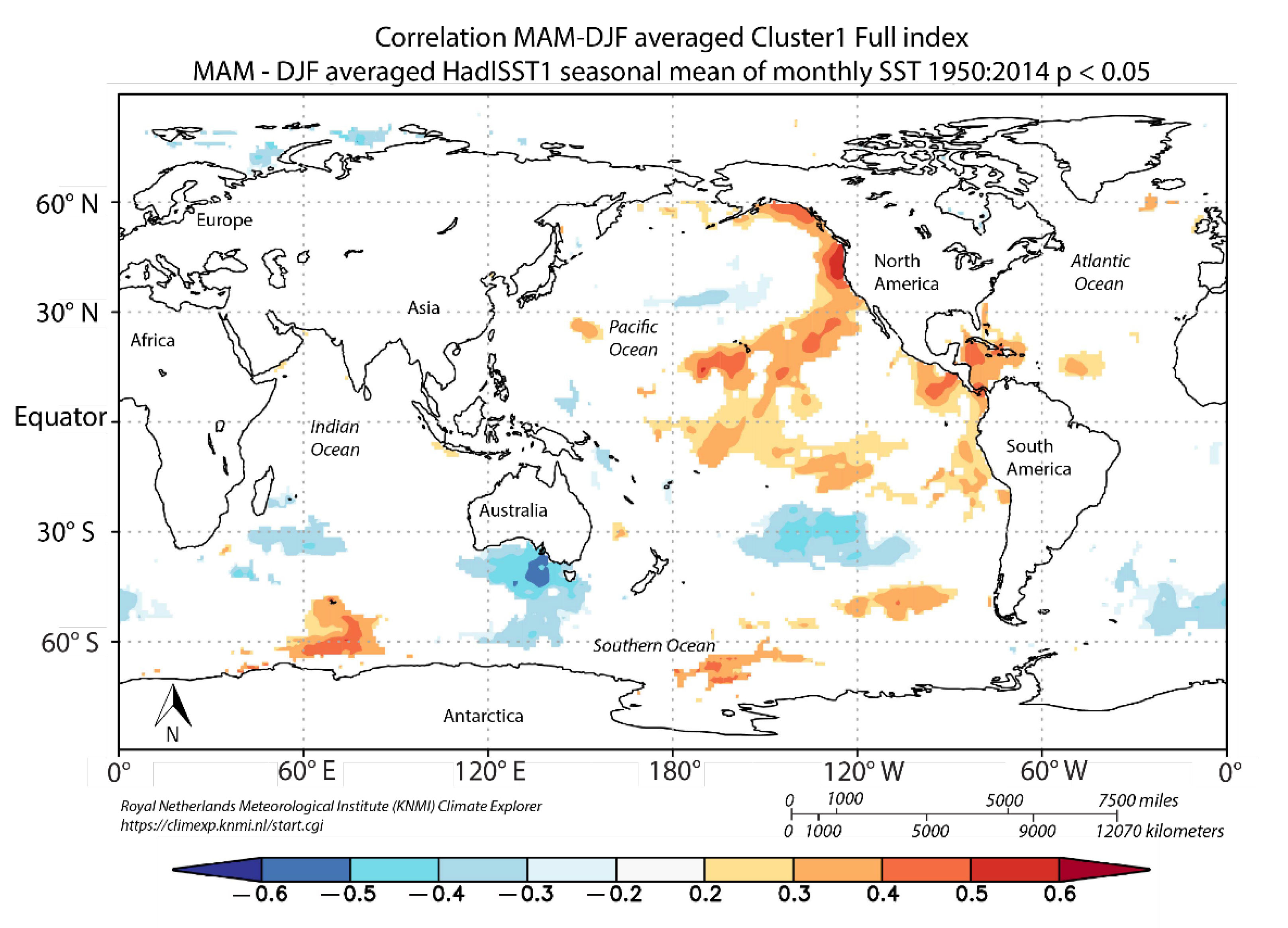
4.2. Correlation between Seasonal Time-Series of Cluster-Mean Streamflow and Climate Indices
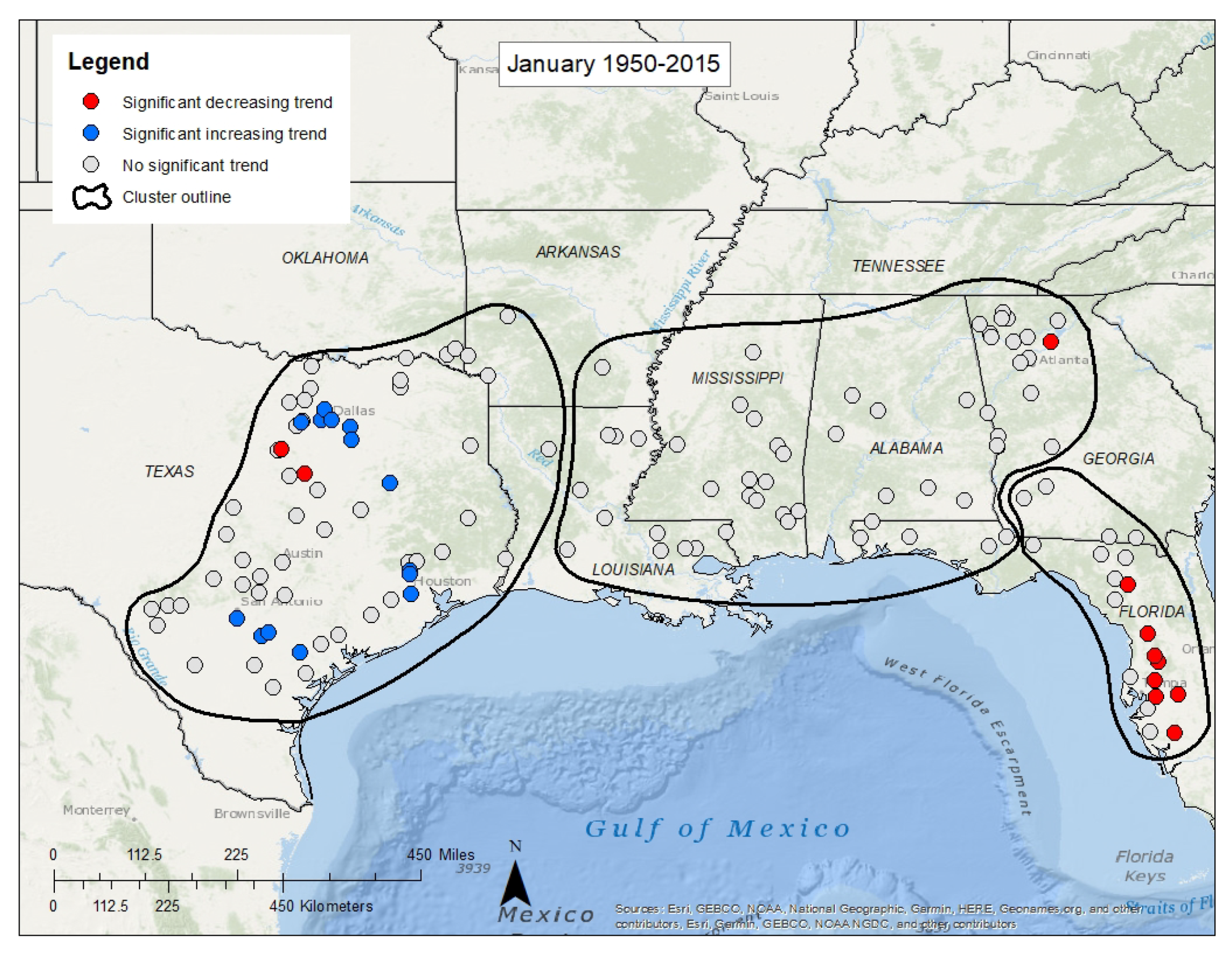
4.3. Trends in Monthly Mean Streamflow
4.4. Trends in Seasonal Mean Streamflow
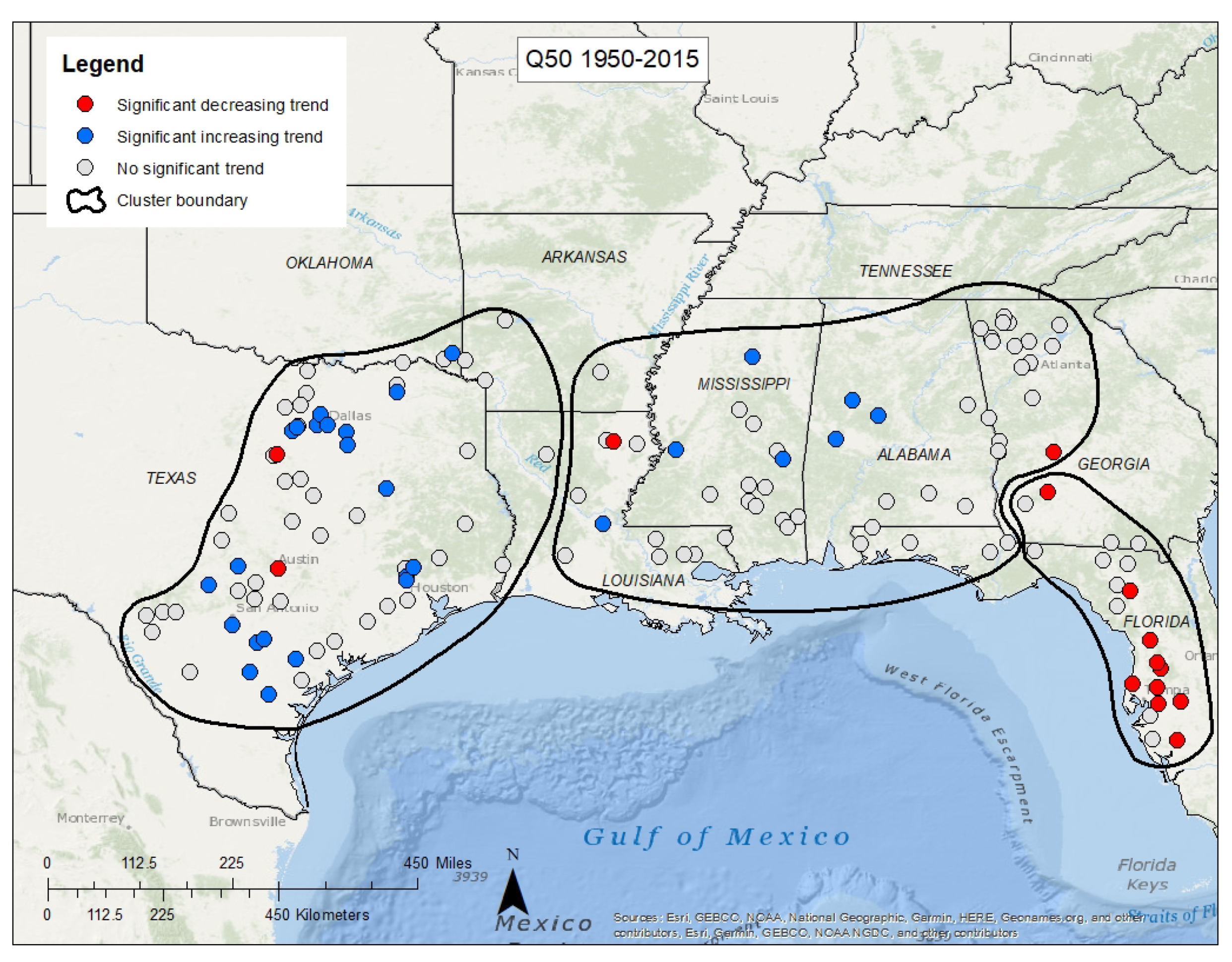
4.5. Trends in 11 Deciles of Annual Streamflow at 139 Streamflow-Gaging Stations
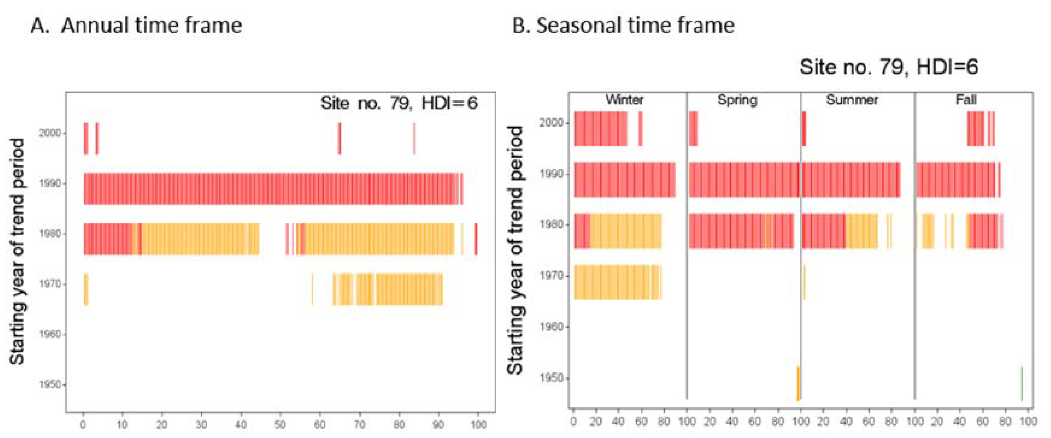
4.6. Trends in the Full Range of Streamflow Quantiles (Quantile-Kendall Analysis)
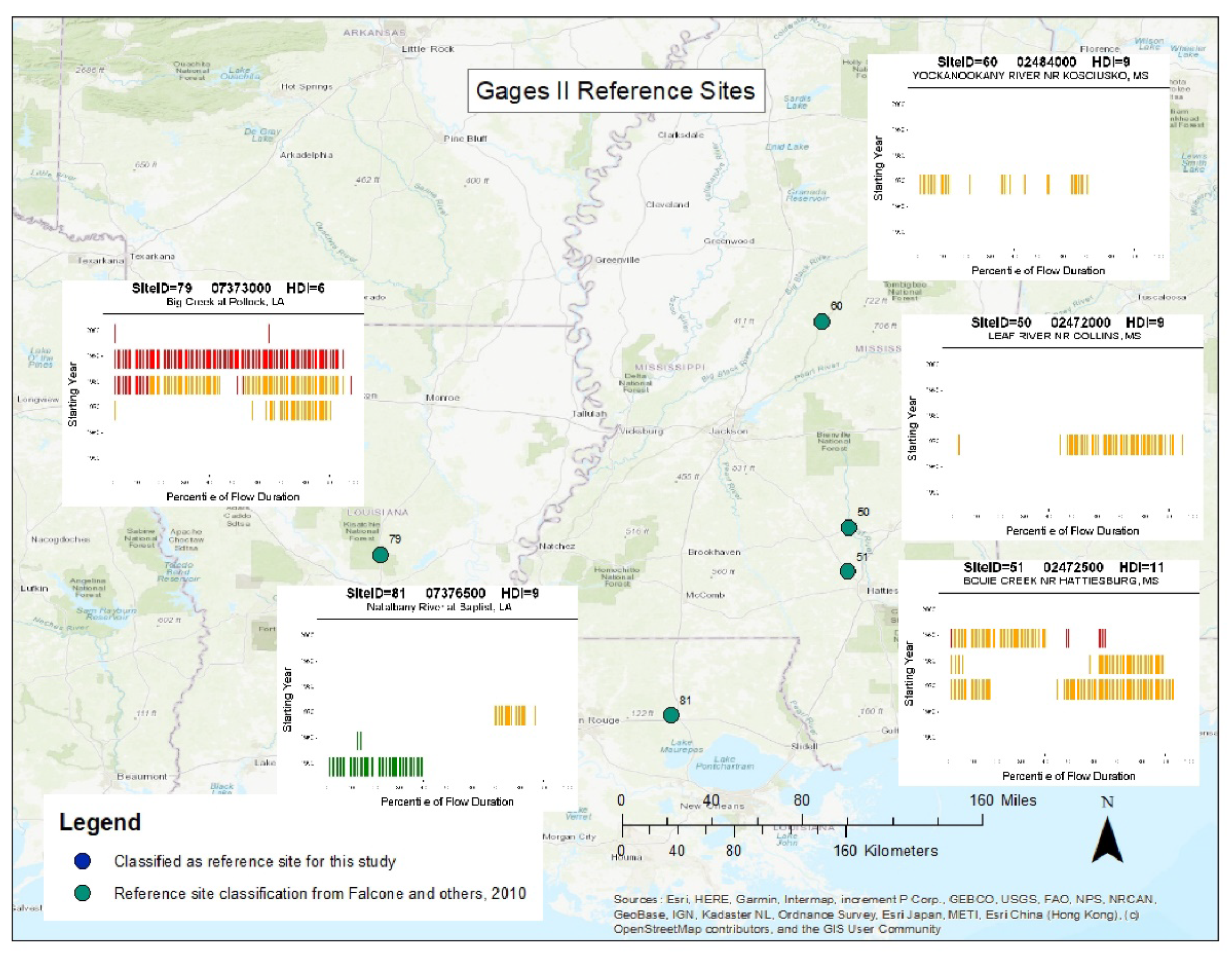
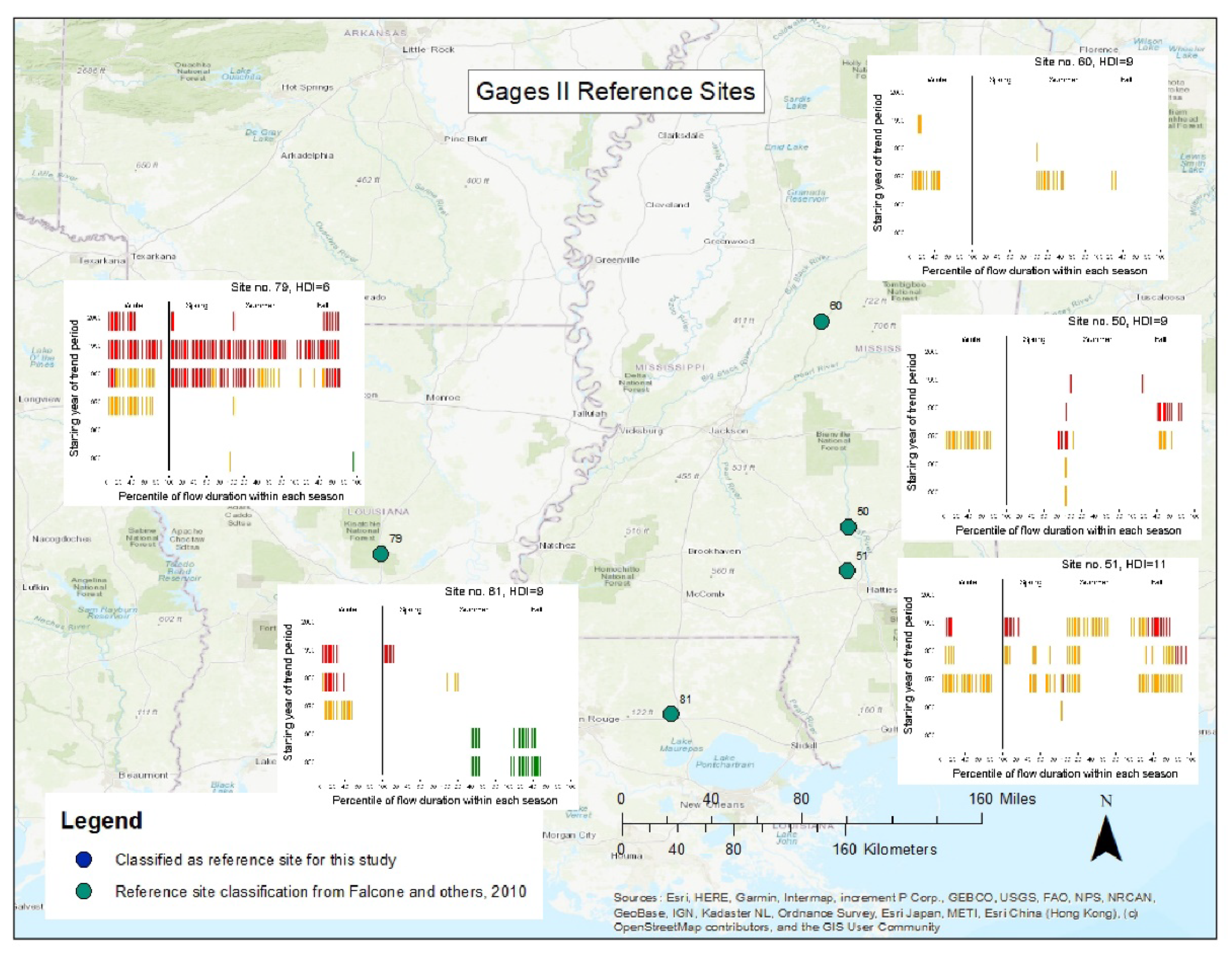
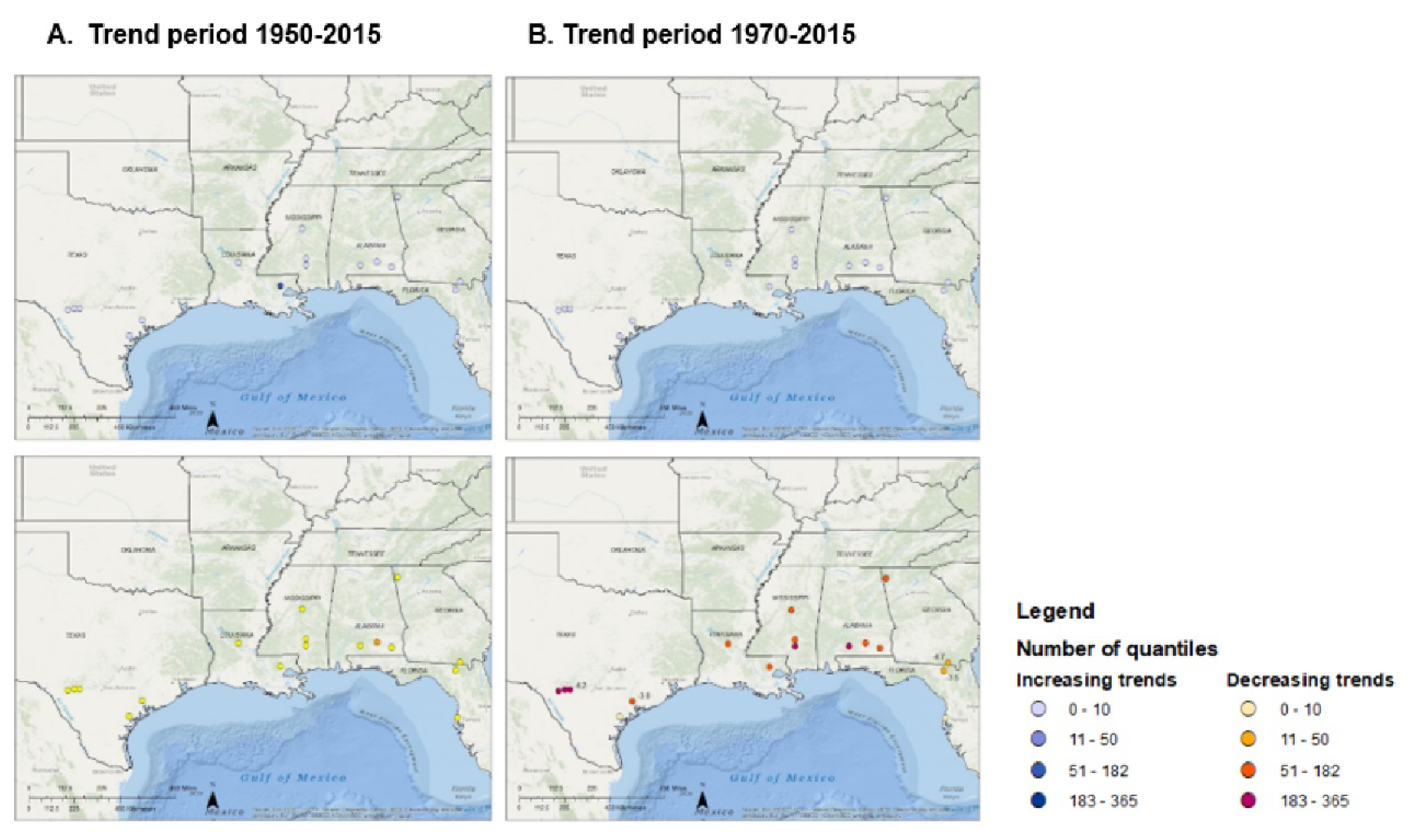
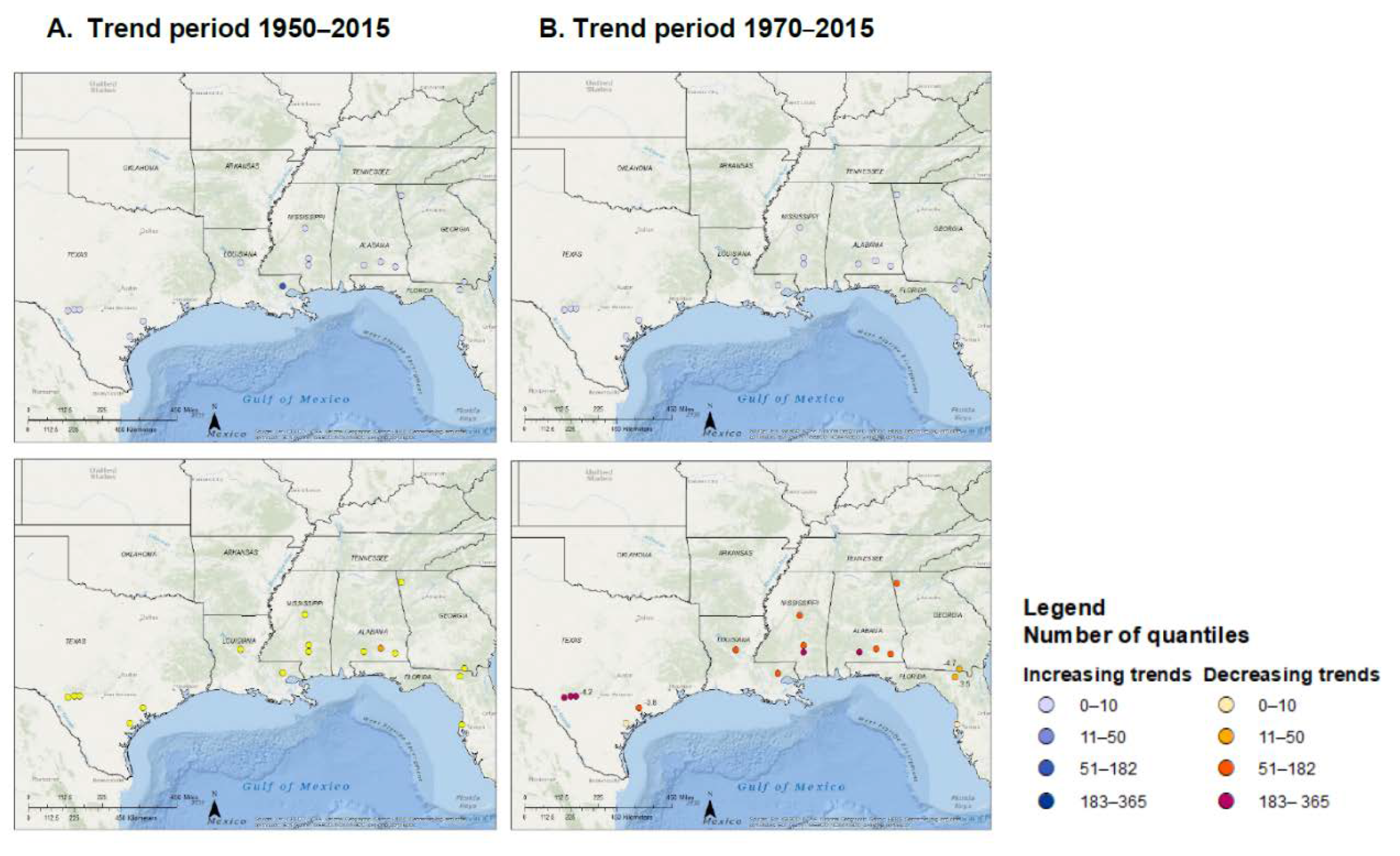
4.7. Spatial Variation in Streamflow Quantile Trends for Reference Sites (Reflecting Temporal Variation in Climate)
- Steepness of trends: Clusters 1, 2, and 3 (Supplementary Materials S2) have very few significant trends, but the slopes of the trends are steep (>2% change per year). In cluster 4, closer to the coast, the significant trends for longer trend periods tend to be shallow, whereas the slopes of significant trends for shorter, more recent trend periods (1980–2015 and 1990–2015) tend to be steeper. This is especially evident in the results of the seasonally stratified Q-K (likely due to the same factors that caused fewer significant trends for longer periods). In cluster 5, all slopes of significant trends are steep.
- Number of significant decreasing trends in higher streamflows (Supplementary Materials S2): Almost no trends in high streamflows were identified for sites in clusters 1, 2, and 3. Trends in high streamflow were present at some (5) sites in cluster 4, and in cluster 5 all reference sites show decreasing trends in high streamflows.
- Occurrence of trends in summer and fall streamflows (Supplementary Materials S2): Every reference site in cluster 5 had a significant decreasing trend in fall streamflow. Perhaps the dominance of precipitation (as high as 70% of the annual total) during warmer months and the resultant evapotranspiration combined with water use in this region makes streamflow more sensitive to changes in climate, hence steeper slopes, and more significant trends.
4.8. Spatial Variation in Streamflow Quantile Trends for Non-Reference Sites
4.9. Departure of Trend Results from Climate-Driven Conditions
5. Conclusions
Supplementary Materials
Author Contributions
Funding
Acknowledgments
Conflicts of Interest
References
- Lorenz, D.L.; Diekoff, A.L. smwrGraphs—An R package for graphing hydrologic data, version 1.1.2. Open-File Rep. 2017, 26, 227–230. [Google Scholar] [CrossRef]
- Lettenmaier, D.P.; Wood, E.F.; Wallis, J.R. Hydro-Climatological Trends in the Continental United States, 1948–1988. J. Clim. 1994, 7, 586–607. [Google Scholar] [CrossRef]
- Peterson, T.C.; Heim, R.R., Jr. Monitoring and understanding changes in heat waves, cold waves, floods, and droughts in the United States: State of knowledge. Bull. Am. Meteorol. Soc. 2013, 6, 821–834. [Google Scholar] [CrossRef]
- Knight, R.; Murphy, J.C.; Wolfe, W.J.; Saylor, C.F.; Wales, A.K. Ecological limit functions relating fish community response to hydrologic departures of the ecological flow regime in the Tennessee River basin, United States. Ecohydrology 2014, 7, 1262–1280. [Google Scholar] [CrossRef]
- Ruhí, A.; Olden, J.D.; Sabo, J.L. Declining streamflow induces collapse and replacement of native fish in the American Southwest. Front. Ecol. Environ. 2016, 14, 465–472. [Google Scholar] [CrossRef]
- Rice, J.S.; Emanuel, R.E.; Vose, J.M.; Nelson, S.A.C. Continental U.S. streamflow trends from 1940 to 2009 and their relationships with watershed spatial characteristics. Water Resour. Res. 2015, 51, 6262–6275. [Google Scholar] [CrossRef]
- McCabe, G.J.; Wolock, D.M. Spatial and temporal patterns in conterminous United States streamflow characteristics. Geophys. Res. Lett. 2014, 41, 6889–6897. [Google Scholar] [CrossRef]
- Sagarika, S.; Kalra, A.; Ahmad, S. Evaluating the effect of persistence on long-term trends and analyzing step changes in streamflows of the continental United States. J. Hydrol. 2014, 517, 36–53. [Google Scholar] [CrossRef]
- Dettinger, M.D.; Diaz, H.F. Global Characteristics of Stream Flow Seasonality and Variability. J. Hydrometeorol. 2000, 1, 289–310. [Google Scholar] [CrossRef]
- Döll, P.; Schmied, H.M. How is the impact of climate change on river flow regimes related to the impact on mean annual runoff? A global-scale analysis. Environ. Res. Lett. 2012, 7, 014037. [Google Scholar] [CrossRef]
- Milly, P.C.D.; Betancourt, J.; Falkenmark, M.; Hirsch, R.M.; Kundzewicz, Z.W.; Lettenmaier, D.P.; Stouffer, R.J. Stationarity Is Dead: Whither Water Management? Science 2008, 319, 573–574. [Google Scholar] [CrossRef] [PubMed]
- Bates, B.C.; Hope, P.; Ryan, B.; Smith, I.; Charles, S. Key findings from the Indian Ocean Climate Initiative and their impact on policy development in Australia. Clim. Chang. 2008, 89, 339–354. [Google Scholar] [CrossRef]
- Cayan, D.R.; Webb, R.H. El Nino/Southern Oscillation and Streamflow in the Western U.S. Historical and Paleoclimatic Aspects of the Southern Oscillation; Diaz, H.F., Markgraf, V., Eds.; Cambridge University Press: Cambridge, UK, 1992; pp. 29–68. [Google Scholar]
- Coleman, J.; Budikova, D. Eastern U.S. summer streamflow during extreme phases of the North Atlantic oscillation. J. Geophys. Res. Atmos. 2013, 118, 4181–4193. [Google Scholar] [CrossRef]
- Cayan, D.R.; Peterson, D.H. The Influence of North Pacific Atmospheric Circulation on Streamflow in the West. In Flood Damage Survey and Assessment; American Geophysical Union (AGU): Washington, DC, USA, 2013; pp. 375–397. [Google Scholar]
- National Oceanic and Atmospheric Administration. “Drought Monitoring.” National Oceanic and Atmospheric Administration. Available online: https://www.ncdc.noaa.gov/temp-and-precip/drought/ (accessed on 30 April 2019).
- Schulte, J.A.; Najjar, R.G.; Li, M. The influence of climate modes on streamflow in the Mid-Atlantic region of the United States. J. Hydrol. Reg. Stud. 2016, 5, 80–99. [Google Scholar] [CrossRef]
- Mantua, N.J.; Hare, S.; Zhang, Y.; Wallace, J.M.; Francis, R.C. A Pacific multi-decadal climate oscillation with impacts on salmon production. Bull. Am. Meteorol. Soc. 1997, 78, 1069–1079. [Google Scholar] [CrossRef]
- Kahya, E.; Dracup, J.A. The Influences of Type 1 El Niño and La Niña Events on Streamflows in the Pacific Southwest of the United States. J. Clim. 1994, 7, 965–976. [Google Scholar] [CrossRef]
- McCabe, G.J.; Dettinger, M.D. Primary Modes and Predictability of Year-to-Year Snowpack Variations in the Western United States from Teleconnections with Pacific Ocean Climate. J. Hydrometeorol. 2002, 3, 13–25. [Google Scholar] [CrossRef]
- Milly, P.C.D.; Dunne, K.A.; Vecchia, A.V. Global pattern of trends in streamflow and water availability in a changing climate. Nat. Cell Biol. 2005, 438, 347–350. [Google Scholar] [CrossRef]
- Krakauer, N.Y.; Fung, I. Mapping and attribution of change in streamflow in the conterminous United States: Hydrol. Earth Syst. Sci. 2008, 12, 1111–1120. Available online: https://www.hydrol-earth-syst-sci.net/12/1111/2008/hess-12-1111-2008.pdf (accessed on 2 May 2019). [CrossRef]
- McCabe, G.J.; Wolock, D. Trends and temperature sensitivity of moisture conditions in the conterminous United States. Clim. Res. 2002, 20, 19–29. [Google Scholar] [CrossRef]
- McCabe, G.J.; Wolock, D.M. A step increase in streamflow in the conterminous United States. Geophys. Res. Lett. 2002, 29, 38-1. [Google Scholar] [CrossRef]
- Hirsch, R.M.; De Cicco, L. User guide to Exploration and Graphics for RivEr Trends (EGRET) and dataRetrieval: R packages for hydrologic data. Tech. Methods 2015. [Google Scholar] [CrossRef]
- Yu, G.; Wright, D.B.; Zhu, Z.; Smith, C.; Holman, K.D. Process-based flood frequency analysis in an agricultural watershed exhibiting nonstationary flood seasonality. Hydrol. Earth Syst. Sci. 2019, 23, 2225–2243. [Google Scholar] [CrossRef]
- Choquette, A.; Hirsch, R.; Murphy, J.; Johnson, L.; Confesor, R. Tracking changes in nutrient delivery to western Lake Erie: Approaches to compensate for variability and trends in streamflow. J. Great Lakes Res. 2019, 45, 21–39. [Google Scholar] [CrossRef]
- Falcone, J.A.; Carlisle, D.M.; Wolock, D.; Meador, M.R. GAGES: A stream gage database for evaluating natural and altered flow conditions in the conterminous United States. Ecology 2010, 91, 621. [Google Scholar] [CrossRef]
- Seaber, P.R.; Kapinos, F.P.; Knapp, G.L. Hydrologic Unit Maps, U.S. Geological Survey Water Supply Paper 2294. 1987. Available online: https://pubs.usgs.gov/wsp/wsp2294/pdf/wsp_2294.pdf (accessed on 5 October 2017).
- United States Census Bureau/American FactFinder. “P12: Sex by Age.” 2010 Census.U.S. Census Bureau. 2010. Available online: https//data.census.gov/cedsci/ (accessed on 1 January 2013).
- Dieter, C.A.; Maupin, M.A.; Caldwell, R.R.; Harris, M.A.; Ivahnenko, T.I.; Lovelace, J.K.; Barber, N.L.; Linsey, K.S. Estimated use of water in the United States in 2015. Circular 2018, 1441. [Google Scholar] [CrossRef]
- United States Department of Agriculture. Southeastern Climate [factsheet]. 2020. Available online: https://www.climatehubs.usda.gov/sites/default/files/SERCH_SEClimate_Factsheet.pdf (accessed on 1 June 2018).
- Omernik, J.M.; Griffith, G.E. Ecoregions of the Conterminous United States: Evolution of a Hierarchical Spatial Framework. Environ. Manag. 2014, 54, 1249–1266. [Google Scholar] [CrossRef]
- Fenneman, N.M. Physiography of Eastern United States. Geogr. J. 1938, 92, 470. [Google Scholar] [CrossRef]
- Horton, J.D.; Juan, C.A.S.; Stoeser, D.B. The State Geologic Map Compilation (SGMC) geodatabase of the conterminous United States. Data Ser. 2017, 1–46. [Google Scholar] [CrossRef]
- Köppen, W. Das geographische System der Klimate. In Handbuch der Klimatologie; Köppen, W., Geiger, R., Eds.; Gebrüder Borntraeger: Berlin, Germany, 1936; pp. C1–C44. Available online: http://koeppen-geiger.vu-wien.ac.at/pdf/Koppen_1936.pdf (accessed on 18 August 2018).
- Arguez, A.; Durre, I.; Applequist, S.; Vose, R.S.; Squires, M.F.; Yin, X.; Heim, R.R.; Owen, T.W. NOAA’s 1981–2010 U.S. Climate Normals: An Overview. Bull. Am. Meteorol. Soc. 2012, 93, 1687–1697. [Google Scholar] [CrossRef]
- U.S. Geological Survey. USGS Water Data for the Nation: U.S. Geological Survey National Water Information System Database. 2016. Available online: http://dx.doi.org/10.5066/F7P55KJN (accessed on 20 June 2012).
- Helsel, D.R.; Hirsch, R.M. Statistical Methods in Water Resources; Elsevier Science Publishing Co.: New York, NY, USA, 1992; 522p. Available online: https://pubs.usgs.gov/twri/twri4a3/pdf/twri4a3-new.pdf (accessed on 1 March 2017).
- Trouet, V.; Van Oldenborgh, G.J. KNMI Climate Explorer: A Web-Based Research Tool for High-Resolution Paleoclimatology. Tree-Ring Res. 2013, 69, 3–13. [Google Scholar] [CrossRef]
- Rayner, N.A.; Parker, D.E.; Horton, E.B.; Folland, C.K.; Alexander, L.V.; Rowell, D.P.; Kent, E.C.; Kaplan, A.L. Global analyses of sea surface temperature, sea ice, and night marine air temperature since the late nineteenth century. J. Geophys. Res. Space Phys. 2003, 108, 4407. [Google Scholar] [CrossRef]
- National Weather Service Climate Prediction Center. North Atlantic Oscillation. Available online: https://www.cpc.ncep.noaa.gov/products/precip/CWlink/pna/nao.shtml (accessed on 26 October 2018).
- Kennedy, J.J.; Rayner, N.A.; Atkinson, C.P.; Killick, R.E. An Ensemble Data Set of Sea Surface Temperature Change From 1850: The Met Office Hadley Centre HadSST.4.0.0.0 Data Set. J. Geophys. Res. Atmos. 2019, 124, 7719–7763. [Google Scholar] [CrossRef]
- National Weather Service Climate Prediction Center. Pacific-North American Pattern. Available online: https://www.cpc.ncep.noaa.gov/products/precip/CWlink/pna/pna.shtml (accessed on 26 October 2018).
- Mann, H.B. Nonparametric Tests Against Trend. Econometric 1945, 13, 245. [Google Scholar] [CrossRef]
- Kendall, M.G. Rank Correlation Methods, 4th ed.; Charles Griffin: London, UK, 1975. [Google Scholar]
- Sen, P.K. Estimates of the regression coefficient based on Kendall’s tau. J. Am. Stat. Assoc. 1968, 63, 1379–1389. [Google Scholar] [CrossRef]
- Thiel, H. A rank-invariant method of linear and polynomial regression analysis, part 3. In Proceedings of the Koninklijke Nederlandse Akademie Wetenschappen; Series A Mathematical Sciences; Royal Netherlands Academy of Arts and Sciences: Amsterdam, The Netherlands, 1950; Volume 53, pp. 1397–1412. [Google Scholar]
- Rodgers, K.D.; Hoos, A.B.; Roland, V.L.; Knight, R.R. Trend Analysis Results for Sites Used in RESTORE Streamflow Alteration Assessments (ver. 1.1, November 2019): U.S. Geological Survey Data Release. 2018. Available online: https://doi.org/10.5066/P9YSE754 (accessed on 1 November 2019).
- Ross, T.F.; Lott, N.; McCown, S.; Quinn, D. The El Nino winter of ’97–’98. National Climatic Data Center Technical Report. 1998, pp. 98–102. Available online: https://www.semanticscholar.org/paper/The-El-Nino-winter-of-’97-’98-Ross-Lott/f7feb92617fe78d270d7b52d469fb3bdb0663072 (accessed on 1 November 2019).
- Rajagopalan, B.; Cook, E.; Lall, U.; Ray, B.K. Spatiotemporal Variability of ENSO and SST Teleconnections to Summer Drought over the United States during the Twentieth Century. J. Clim. 2000, 13, 4244–4255. [Google Scholar] [CrossRef]
- Tootle, G.A.; Piechota, T.C.; Singh, A. Coupled oceanic-atmospheric variability and U.S. streamflow. Water Resour. Res. 2005, 41. [Google Scholar] [CrossRef]
- Juanxiong, H.; Zhihao, Y.; Yang, X. Temporal Characteristics of Pacific Decadal Oscillation (PDO) and ENSO and Their Relationship Analyzed with Method of Empirical Mode Decomposition (EMD). Acta Meteorol. Sin. 2005, 19, 83. [Google Scholar]
- Hamlet, A.F.; Lettenmaier, D.P. Columbia River Streamflow Forecasting Based on ENSO and PDO Climate Signals. J. Water Resour. Plan. Manag. 1999, 125, 333–341. [Google Scholar] [CrossRef]
- Gershunov, A.; Barnett, T.P.; Cayan, D.R. North Pacific interdecadal oscillation seen as factor in ENSO-related North American climate anomalies. Eos 1999, 80, 25. [Google Scholar] [CrossRef]
- Allan, R.; Reason, C.; Lindesay, J.; Ansell, T. Protracted’ ENSO episodes and their impacts in the Indian Ocean region. Deep. Sea Res. Part II Top. Stud. Oceanogr. 2003, 50, 2331–2347. [Google Scholar] [CrossRef]
- Verdon, D.C.; Franks, S.W. Long-term behaviour of ENSO: Interactions with the PDO over the past 400 years inferred from paleoclimate records. Geophys. Res. Lett. 2006, 33, 6712. [Google Scholar] [CrossRef]
- Enfield, D.B.; Mestas-Nuñez, A.M.; Trimble, P.J. The Atlantic Multidecadal Oscillation and its relation to rainfall and river flows in the continental U.S. Geophys. Res. Lett. 2001, 28, 2077–2080. [Google Scholar] [CrossRef]
- Sanks, K.M.; Rodgers, K.D. Trend Departure Index Results for Sites in the RESTORE Trend Analysis and Hydrologic Alteration Studies: U.S. Geological Survey Data Release. 2020. Available online: https://doi.org/10.5066/P9ASCZER (accessed on 1 October 2020).


| Kendall’s Tau | p-Value | Sen’s Slope Estimate | Sen’s Slope C.I. Upper/Lower | |
|---|---|---|---|---|
| Cluster 1 | −0.118 | 0.004 | −0.001 | −0.0022/−0.0004 |
| Cluster 2 | −0.185 | 0.000 | −0.002 | −0.0029/−0.0012 |
| Cluster 3 | −0.105 | 0.010 | −0.002 | −0.0027/−0.0004 |
| Cluster 4 | 0.009 | 0.819 | 0.000 | −0.0009/0.0012 |
| Cluster 5 | 0.085 | 0.038 | 0.001 | 0.0016/0.00004 |
| Climate Index | Cluster 1 | p-Value | Cluster 2 | p-Value | Cluster 3 | p-Value | Cluster 4 | p-Value | Cluster 5 | p-Value |
|---|---|---|---|---|---|---|---|---|---|---|
| PDO | 0.18 | 0.003 | 0.16 | 0.011 | 0.15 | 0.015 | 0.10 | 0.089 | 0.21 | 0.001 |
| AMO | −0.05 | 0.379 | −0.07 | 0.236 | −0.28 | 0.000 | −0.15 | 0.013 | −0.16 | 0.008 |
| NAO | −0.04 | 0.540 | −0.03 | 0.624 | 0.01 | 0.828 | 0.05 | 0.406 | 0.03 | 0.685 |
| ENSO | 0.23 | 0.00 | 0.16 | 0.008 | 0.20 | 0.001 | 0.11 | 0.072 | 0.22 | 0.00 |
| PNA | 0.20 | 0.001 | 0.15 | 0.018 | 0.12 | 0.051 | −0.03 | 0.663 | 0.18 | 0.003 |
| Cluster | PDO | AMO | NAO | ENSO | PNA |
|---|---|---|---|---|---|
| 1 | 3.25 | 0.3 | 0.14 | 5.3 | 3.97 |
| 2 | 2.42 | 0.54 | 0.09 | 2.62 | 2.13 |
| 3 | 2.25 | 7.63 | 0.02 | 4.09 | 1.45 |
| 4 | 1.1 | 2.36 | 0.26 | 1.23 | 0.07 |
| 5 | 4.26 | 2.65 | 0.06 | 4.8 | 3.28 |
| 1950 | 1960 | 1970 | |||||||||
| Month | Significant Trends | Increasing Trends | Decreasing Trends | Month | Significant Trends | Increasing Trends | Decreasing Trends | Month | Significant Trends | Increasing Trends | Decreasing Trends |
| January | 25 | 14 | 11 | January | 33 | 5 | 28 | January | 35 | 0 | 35 |
| February | 21 | 7 | 14 | February | 36 | 2 | 34 | February | 35 | 0 | 35 |
| March | 44 | 29 | 15 | March | 38 | 8 | 30 | March | 27 | 2 | 25 |
| April | 29 | 11 | 18 | April | 26 | 3 | 23 | April | 21 | 1 | 20 |
| May | 26 | 4 | 22 | May | 34 | 2 | 32 | May | 42 | 0 | 42 |
| June | 20 | 9 | 11 | June | 34 | 2 | 32 | June | 34 | 0 | 34 |
| July | 29 | 17 | 12 | July | 37 | 9 | 28 | July | 16 | 5 | 11 |
| August | 36 | 23 | 13 | August | 41 | 3 | 38 | August | 57 | 9 | 48 |
| September | 31 | 19 | 12 | September | 34 | 8 | 26 | September | 37 | 5 | 32 |
| October | 33 | 20 | 13 | October | 29 | 5 | 24 | October | 24 | 1 | 23 |
| November | 36 | 23 | 13 | November | 22 | 8 | 14 | November | 19 | 3 | 16 |
| December | 25 | 17 | 8 | December | 17 | 3 | 14 | December | 21 | 1 | 20 |
| 1980 | 1990 | 2000 | |||||||||
| Month | Significant Trends | Increasing Trends | Decreasing Trends | Month | Significant Trends | Increasing Trends | Decreasing Trends | Month | Significant Trends | Increasing Trends | Decreasing Trends |
| January | 12 | 0 | 12 | January | 39 | 0 | 39 | January | 15 | 3 | 12 |
| February | 19 | 0 | 19 | February | 44 | 0 | 44 | February | 21 | 0 | 21 |
| March | 14 | 0 | 14 | March | 42 | 0 | 42 | March | 11 | 0 | 11 |
| April | 7 | 1 | 6 | April | 27 | 0 | 27 | April | 5 | 0 | 5 |
| May | 14 | 0 | 14 | May | 15 | 0 | 15 | May | 4 | 3 | 1 |
| June | 21 | 0 | 21 | June | 24 | 1 | 23 | June | 1 | 0 | 1 |
| July | 12 | 3 | 9 | July | 22 | 4 | 18 | July | 4 | 1 | 3 |
| August | 15 | 2 | 13 | August | 36 | 1 | 35 | August | 10 | 0 | 10 |
| September | 14 | 2 | 12 | September | 26 | 0 | 26 | September | 13 | 0 | 13 |
| October | 16 | 0 | 16 | October | 20 | 0 | 20 | October | 7 | 0 | 7 |
| November | 24 | 0 | 24 | November | 31 | 0 | 31 | November | 14 | 0 | 14 |
| December | 18 | 0 | 18 | December | 30 | 0 | 30 | December | 24 | 0 | 24 |
| 1950 | 1960 | 1970 | |||||||||
| Season | Significant Trends | Increasing Trends | Decreasing Trends | Season | Significant Trends | Increasing Trends | Decreasing Trends | Season | Significant Trends | Increasing Trends | Decreasing Trends |
| Spring | 25 | 9 | 16 | Spring | 34 | 3 | 31 | Spring | 29 | 1 | 28 |
| Summer | 23 | 12 | 11 | Summer | 36 | 7 | 29 | Summer | 41 | 2 | 39 |
| Fall | 48 | 30 | 18 | Fall | 36 | 11 | 25 | Fall | 27 | 2 | 25 |
| Winter | 22 | 11 | 11 | Winter | 32 | 3 | 29 | Winter | 34 | 1 | 33 |
| 1980 | 1990 | 2000 | |||||||||
| Season | Significant Trends | Increasing Trends | Decreasing Trends | Season | Significant Trends | Increasing Trends | Decreasing Trends | Season | Significant Trends | Increasing Trends | Decreasing Trends |
| Spring | 6 | 0 | 6 | Spring | 29 | 0 | 29 | Spring | 2 | 0 | 2 |
| Summer | 14 | 1 | 13 | Summer | 32 | 1 | 31 | Summer | 3 | 0 | 3 |
| Fall | 17 | 1 | 16 | Fall | 28 | 0 | 28 | Fall | 15 | 0 | 15 |
| Winter | 16 | 0 | 16 | Winter | 39 | 0 | 39 | Winter | 20 | 1 | 19 |
| 1950 | 1960 | 1970 | |||||||||
| Decile | Significant Trends | Increasing Trends | Decreasing Trends | Decile | Significant Trends | Increasing Trends | Decreasing Trends | Decile | Significant Trends | Increasing Trends | Decreasing Trends |
| Q00 | 70 | 35 | 35 | Q00 | 77 | 28 | 49 | Q00 | 82 | 16 | 66 |
| Q10 | 61 | 32 | 29 | Q10 | 72 | 24 | 48 | Q10 | 78 | 13 | 65 |
| Q20 | 49 | 29 | 20 | Q20 | 63 | 20 | 43 | Q20 | 79 | 10 | 69 |
| Q30 | 48 | 31 | 17 | Q30 | 56 | 16 | 40 | Q30 | 66 | 6 | 60 |
| Q40 | 45 | 29 | 16 | Q40 | 49 | 12 | 37 | Q40 | 68 | 5 | 63 |
| Q50 | 42 | 28 | 14 | Q50 | 44 | 10 | 34 | Q50 | 60 | 5 | 55 |
| Q60 | 31 | 18 | 13 | Q60 | 38 | 7 | 31 | Q60 | 55 | 3 | 52 |
| Q70 | 39 | 27 | 12 | Q70 | 36 | 7 | 29 | Q70 | 50 | 2 | 48 |
| Q80 | 27 | 16 | 11 | Q80 | 29 | 5 | 24 | Q80 | 41 | 1 | 40 |
| Q90 | 22 | 13 | 9 | Q90 | 24 | 3 | 21 | Q90 | 27 | 1 | 26 |
| Q100 | 31 | 9 | 22 | Q100 | 28 | 3 | 25 | Q100 | 21 | 2 | 19 |
| 1980 | 1990 | 2000 | |||||||||
| Decile | Significant Trends | Increasing Trends | Decreasing Trends | Decile | Significant Trends | Increasing Trends | Decreasing Trends | Decile | Significant Trends | Increasing Trends | Decreasing Trends |
| Q00 | 50 | 8 | 42 | Q00 | 51 | 5 | 46 | Q00 | 21 | 0 | 21 |
| Q10 | 37 | 6 | 31 | Q10 | 66 | 4 | 62 | Q10 | 22 | 0 | 22 |
| Q20 | 39 | 4 | 35 | Q20 | 61 | 1 | 60 | Q20 | 24 | 0 | 24 |
| Q30 | 35 | 1 | 34 | Q30 | 59 | 1 | 58 | Q30 | 26 | 0 | 26 |
| Q40 | 34 | 2 | 32 | Q40 | 64 | 0 | 64 | Q40 | 26 | 0 | 26 |
| Q50 | 28 | 2 | 26 | Q50 | 63 | 0 | 63 | Q50 | 24 | 0 | 24 |
| Q60 | 26 | 2 | 24 | Q60 | 60 | 0 | 60 | Q60 | 17 | 0 | 17 |
| Q70 | 19 | 1 | 18 | Q70 | 54 | 0 | 54 | Q70 | 12 | 2 | 10 |
| Q80 | 14 | 1 | 13 | Q80 | 46 | 1 | 45 | Q80 | 9 | 3 | 6 |
| Q90 | 8 | 1 | 7 | Q90 | 25 | 1 | 24 | Q90 | 4 | 0 | 4 |
| Q100 | 6 | 1 | 5 | Q100 | 17 | 0 | 17 | Q100 | 3 | 1 | 2 |
| Reference Sites | |||||||||
| Increasing Trends | Decreasing Trends | ||||||||
| Count of quantiles with trends | Count of quantile with trends | ||||||||
| Cluster | Number of sites | Average per site | Standard deviation | Average slope, in percent | Average per site | Standard deviation | Average slope, in percent | ||
| 1 | --a | --a | --a | --a | --a | --a | --a | ||
| 2 | 1 | 0 | --b | --c | 0 | --b | --c | ||
| 3 | 2 | 0 | 0 | --c | 17 | 6 | −4.07 | ||
| 4 | 3 | 0 | 0 | --c | 150 | 95 | −1.11 | ||
| 5 | 5 | 0 | 0 | --c | 190 | 139 | −3.01 | ||
| All | 17 | 0 | 0 | --c | 137 | 115 | −2.07 | ||
| All Sites (excluding spatially dependent sites d) | |||||||||
| Increasing trends | Decreasing trends | Trend Departure Index | |||||||
| Count of quantiles with trends | Count of quantile with trends | ||||||||
| Cluster | Number of sites | Average per site | Standard deviation | Average slope, in percent | Average per site | Standard deviation | Average slope, in percent | Average | Standard deviation |
| 1 | 6 | 3 | 6 | 1 | 18 | 27 | −2.71 | 0.06 | 0.07 |
| 2 | 3 | 0 | 0 | --c | 32 | 52 | −3.10 | 0.09 | 0.14 |
| 3 | 8 | 0 | 0 | --c | 148 | 143 | −2.18 | 0.38 | 0.38 |
| 4 | 49 | 0 | 0 | --c | 130 | 126 | −1.23 | 0.37 | 0.28 |
| 5 | 51 | 15 | 45 | 2.38 | 72 | 118 | −2.79 | 0.68 | 0.41 |
| All | 117 | 7 | 31 | 2.24 | 97 | 123 | −1.91 | 0.48 | 0.39 |
Publisher’s Note: MDPI stays neutral with regard to jurisdictional claims in published maps and institutional affiliations. |
© 2020 by the authors. Licensee MDPI, Basel, Switzerland. This article is an open access article distributed under the terms and conditions of the Creative Commons Attribution (CC BY) license (http://creativecommons.org/licenses/by/4.0/).
Share and Cite
Rodgers, K.; Roland, V.; Hoos, A.; Crowley-Ornelas, E.; Knight, R. An Analysis of Streamflow Trends in the Southern and Southeastern US from 1950–2015. Water 2020, 12, 3345. https://doi.org/10.3390/w12123345
Rodgers K, Roland V, Hoos A, Crowley-Ornelas E, Knight R. An Analysis of Streamflow Trends in the Southern and Southeastern US from 1950–2015. Water. 2020; 12(12):3345. https://doi.org/10.3390/w12123345
Chicago/Turabian StyleRodgers, Kirk, Victor Roland, Anne Hoos, Elena Crowley-Ornelas, and Rodney Knight. 2020. "An Analysis of Streamflow Trends in the Southern and Southeastern US from 1950–2015" Water 12, no. 12: 3345. https://doi.org/10.3390/w12123345
APA StyleRodgers, K., Roland, V., Hoos, A., Crowley-Ornelas, E., & Knight, R. (2020). An Analysis of Streamflow Trends in the Southern and Southeastern US from 1950–2015. Water, 12(12), 3345. https://doi.org/10.3390/w12123345