Machine Learning to Estimate Surface Soil Moisture from Remote Sensing Data

Abstract

Soil moisture is an integral quantity parameter in hydrology and agriculture practices. Satellite remote sensing has been widely applied to estimate surface soil moisture. However, it is still a challenge to retrieve surface soil moisture content (SMC) data in the heterogeneous catchment at high spatial resolution. Therefore, it is necessary to improve the retrieval of SMC from remote sensing data, which is important in the planning and efficient use of land resources. Many methods based on satellite-derived vegetation indices have already been developed to estimate SMC in various climatic and geographic conditions. Soil moisture retrievals were performed using statistical and machine learning methods as well as physical modeling techniques. In this study, an important experiment of soil moisture retrieval for investigating the capability of the machine learning methods was conducted in the early spring season in a semi-arid region of Iran. We applied random forest (RF), support vector machine (SVM), artificial neural network (ANN), and elastic net regression (EN) algorithms to soil moisture retrieval by optical and thermal sensors of Landsat 8 and knowledge of land-use types on previously untested conditions in a semi-arid region of Iran. The statistical comparisons show that RF method provided the highest Nash–Sutcliffe efficiency value (0.73) for soil moisture retrieval covered by the different land-use types. Combinations of surface reflectance and auxiliary geospatial data can provide more valuable information for SMC estimation, which shows promise for precision agriculture applications.

1. Introduction

Soil moisture (SM) is a significant component of the hydrological cycle regulating runoff, vegetation production and evapotranspiration [1]. Soil moisture is a major soil indicator to define and identify agricultural drought. Estimation of soil moisture has applications for identifying early-stage water deficit conditions and evolving drought events for crop yield uncertainty and food security conditions, agricultural insurance, policymaking and decision-making, and crop planning [2,3] especially for the arid and semi-arid parts of the globe. Agricultural drought has a catalytic effect that contributes to social and political conflicts in developing countries [4]. Therefore, soil moisture modeling and monitoring are of increasing interest. Monitoring the spatial and temporal variations of SM is a prerequisite both for mitigating and adapting to climate changes for the sustainability of cropping systems as well as for developing precision agriculture and food security [5,6,7,8,9]. Surface soil moisture is generally referred to the water content of the top ~5–15 cm of the soil layer [10]. Although the water in this thin layer of soil constitutes a minute portion of the global water reserves, it embodies fundamental hydrological, biochemical, physiological, agricultural, and other Earth processes [10,11]. Accurate information about the spatial and temporal variations of surface soil moisture are crucial for policy formulation and land-water management.

Soil moisture can be estimated with field measurements by a range of methods. Among the field soil moisture sensors, dielectric soil-moisture probes are applied in unsaturated soil conditions, including time domain reflectometers (TDR), frequency domain reflectometers (FDR), and capacitance probes (CP) [12,13]. These in situ measurements are the most accurate methods to measure SMC and can also be entirely automated [14]. Installation and maintenance can, however, be very labor-intensive, and measurements are accurate only at the point of measurement [15]. Obtaining SMC estimates from earth observation satellites [10,16,17] and land–atmosphere processes models [18] is thus necessary for acquiring spatial and temporal coverage for, e.g., real-time management and precision agriculture. However, parametric uncertainty and disturbances related to, e.g., atmospheric conditions, vegetation, and surface roughness, are still subjects of investigation for identifying suitable models for estimating SM [14].

The favored source for mapping surface wetness from satellite sensors is optical data. The advantage of using optical data as opposed to active microwave is that a large data archive of high-resolution data exists and is updated to be collected operationally, e.g., series of Landsat observations since 1972 [19]. Moisture content in the soil also affects the spectral reflectance of the soil, however, the manner in which it affects so varies across the electromagnetic spectrum [20]. Theoretically, changes in soil reflectivity occur when air particle interfaces are replaced by liquid–water particle interfaces [21]. Remote sensing in the visible-near infrared (Vis-NIR) spectrum is a less effective spectral domain for soil moisture measurement because of the confounding effects factors [22]. Nevertheless, there have been successful results to apply visible and infrared wavelengths in soil moisture estimation from remote sensing data [20]. The previous results indicate that it is possible to estimate surface soil moisture (0–7.6 cm) from visible and near-infrared reflectance [20]. However, estimating soil moisture regimes rather than precise water content is perhaps more preferred. In this study, we consider the potential combinations of reflectance bands rather than a single band to estimate surface soil moisture, four popular machine learning techniques were performed on the 5-band data set. Also, thermal emissivity data (3.5 and 14 μm) have been used for estimating SMC [13]. The possibility to develop ratios and normalized difference (ND) algorithms for quantitively estimate water content in leaves has been investigated [23,24,25]. A variety of ND indices and biophysical parameters (e.g., leaf area index (LAI)) have been suggested and tested for estimating SMC [26,27,28,29,30], but there are still several unresolved questions regarding the applicability of various reflectance spectra bands (e.g., red, near-infrared (NIR), and short-wave infrared (SWIR) in the optical domain) to estimate SMC directly [29]. Regression methods remain popular because of their simple methodology, long history of application, and successful application to a wide variety of processes by both practitioners and academicians. However, for traditional regression analysis, some statistical assumptions required to be made may lead to limited use, such as outlier data, nonlinearity, heteroscedasticity, and, multicollinearity. Numerous machine learning methods have emerged to overcome the above problems such as neural network, random forest, decision trees. Machine learning refers to automatic or semi-automatic exploration and analysis of large data sets, in order to discover meaningful correlations, patterns, and rules among data [31]. Machine learning approaches are now commonplace which have been successfully applied for predicting soil moisture using remotely sensed data in the semi-arid region [28,32]. However, there are still many special cases of interest in terms of using machine learning in remotely sensed soil moisture products. The development of machine learning (ML) has led to renewed attempts to estimate soil moisture from remote sensing [28,29]. One advantage with SM is that non-traditional spatial data sources, for instance, land-use/cover as existing at the landscape scale [33], can be used in the modeling. ML methods are site-specific and when the model has been calibrated, it can only be applied for similar cases as those used for the calibration phase [10]. However, this type of approach can be an important source of information to estimate soil moisture at unsampled areas and for site-specific applications [34,35].

The agricultural sector plays a strategic role in the economy for arid countries more prone to be sensitive to climate events. In arid regions, droughts are recurring climatic events, often threatening agricultural systems and food security [36,37]. The definition of policies and development of best practices management options for dealing with water stress in such regions require the adoption of scenarios of likely future SM conditions as well as real-time or near real-time monitoring and sharing of SM over extended regions. This can only be achieved by adopting freely available remote sensing data and a model that translates the satellite data to SM estimates with an accuracy that is sufficient to support management. This study attempts to semi operationally assess the spatially and temporally continuous estimates of surface soil moisture content using machine learning models which are formulated for visible, thermal infrared remotely sensed data and easily accessible auxiliary data to support and to improve the framework of agriculture management. The primary goal of this study was to develop an alternative remote-sensed approach with rapid, less expensive, and reliable techniques as opposed to ground-based methods to spatially quantify SM by routinely available satellite imagery. This approach must be repeatable and, ideally, able to provide automated spatiotemporal soil moisture mapping over large areas.

2. Materials and Methods

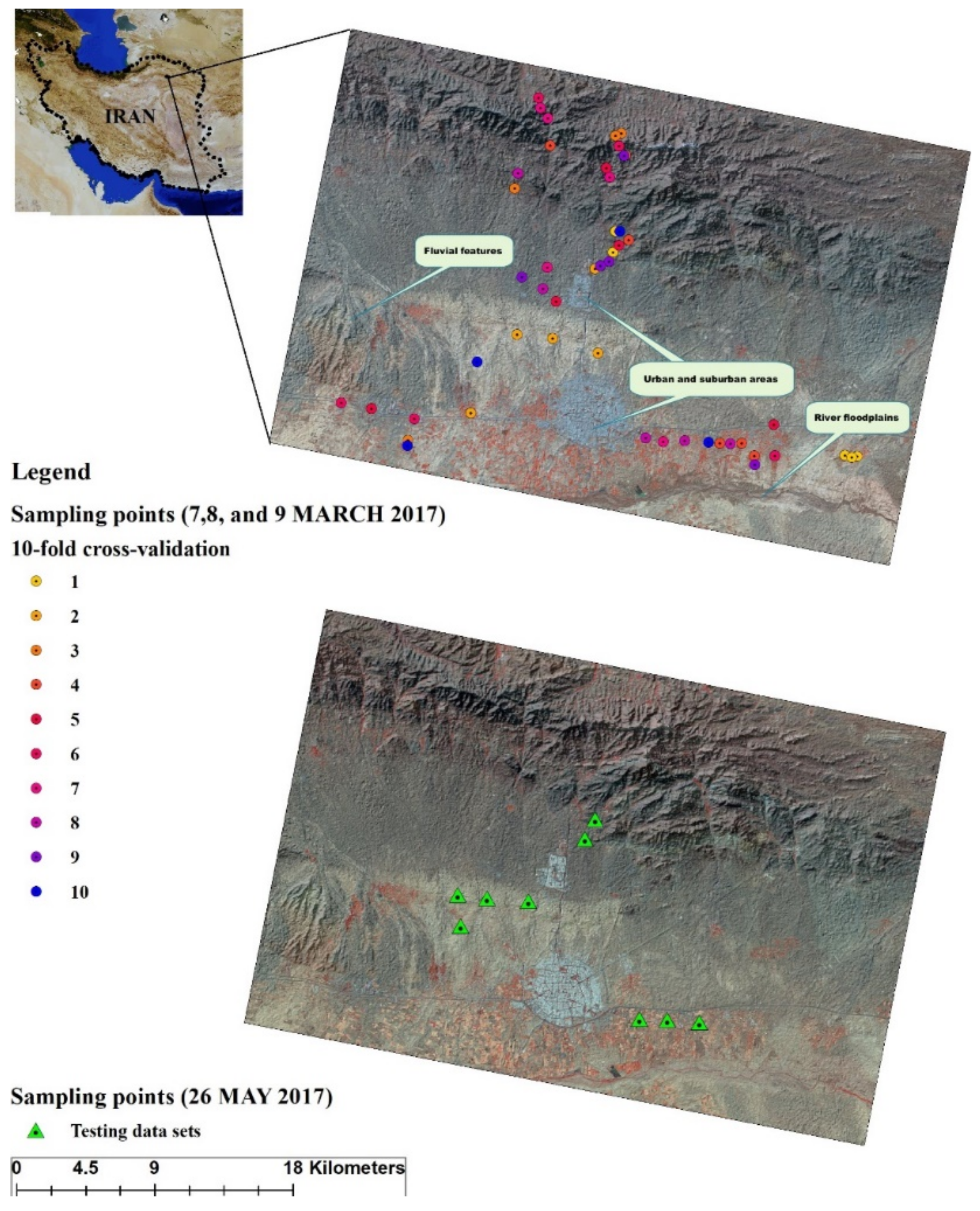
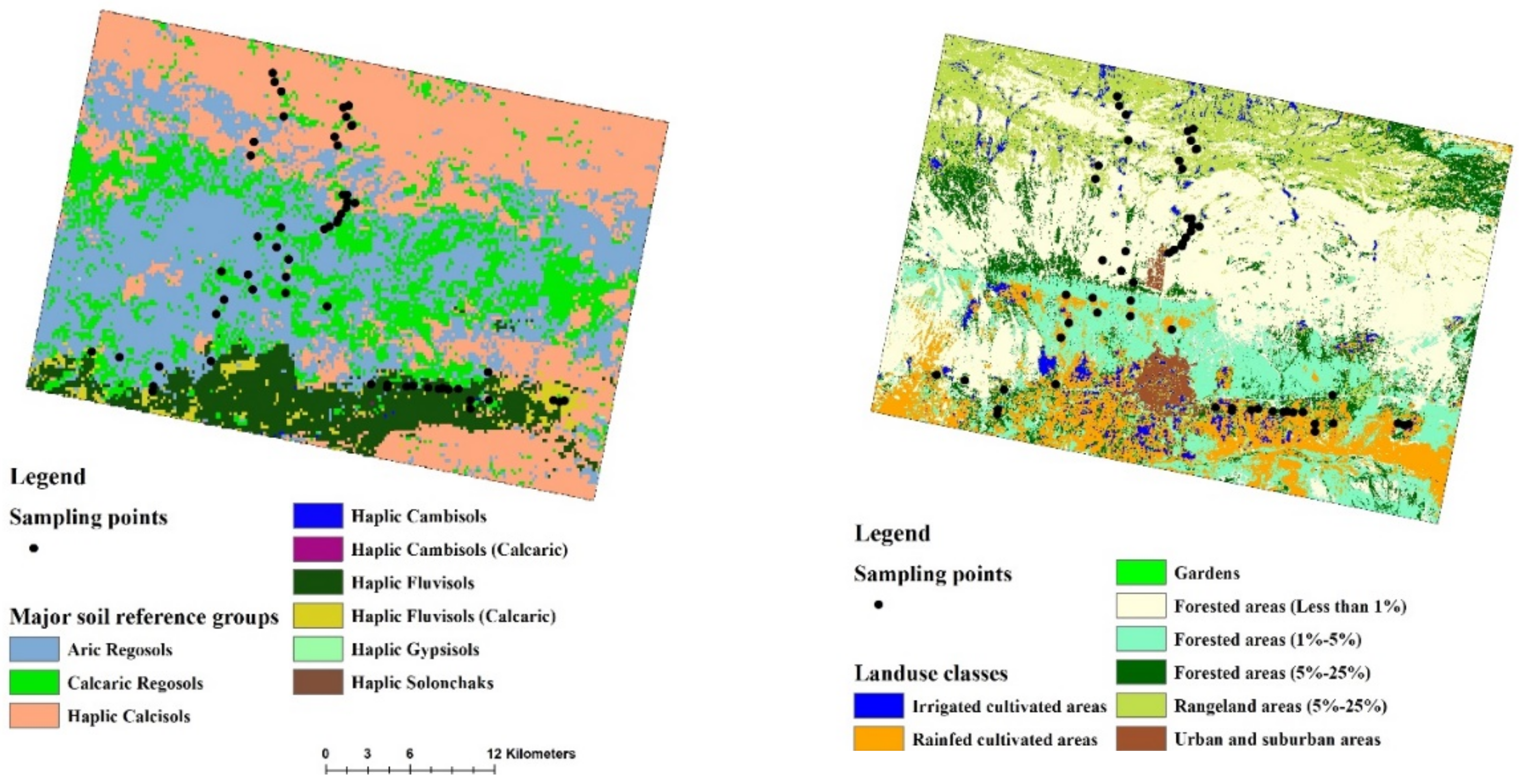
2.1. Study Area

The study area represents the semi-arid region of west Khorasan-Razavi province in Iran (Northeastern), located completely on Quaternary alluvial sediments (Figure 1). The Northeastern semi-arid region also has frequent droughts that can be characterized by the absence of soil moisture information. Droughts are extreme climate events, which often affect SMC in Iran [37]. There were the worst droughts during the period of 1998–2001 and again in 2014 in the Middle-East [38]. The study area includes the Sabzevar county and city, an area of approximately 1100 km² intensively used for residential, semi-industrial, and agricultural purposes. The land-use is mainly forested areas (less than 1% of canopy cover) (42%), agricultural (14%), and settlement (1.5%), and the remaining natural and planted forests of Haloxylon spp, that is a commonly used plant as sand-fixing. The study area is erosion-sensitive and with potential environmental limitations on vegetation and agriculture [39,40,41] and it is mountainous towards the North and large plain characterizes the South; the elevation of the study area varies between 891 and 2085 m, with a mean value of 1229 m above sea level (Figure 1). Although the slope angles vary from 0 to 43 degree, the majority of the terrain is only sloping between 0 and 2 degrees. Long term average annual precipitation at the Sabzevar Weather Station is 188.6 mm. The rainiest month is March with an average of 37 mm while August and September are the driest rainy months (<1 mm). The annual mean air temperature is about 17.4 °C and the average relative air humidity is 41% [42].

2.2. In Situ Soil Moisture Data Collection and Satellite Images

2.2.1. Experimental Design of Soil Samples

Soil moisture in situ measurements were obtained using a portable multi-sensor capacitance probe (PR2, Delta-T Devices Ltd., Cambridge, UK), which can measure volumetric soil moisture (%vol) at six depths: 10, 20, 30, 40, 60, and 100 cm. The PR2 probe has a measure range of 0–100% (m³/m³) and a precision of ±6%; ±0.06 m³/m³ (range of 0 °C to 40 °C) in generalized soil calibration [43]. This sensor was selected n study because of its profile resolution, easy installation, and favorable soil conditions [44]. An important side of soil moisture variability is its effect on the required number of soil samples at different locations to properly estimate the true value of soil moisture through remote sensing data. The experimental design of soil samples (moisture content) is generally based on land-use or soil types in the experiment area [45,46]. For this research, data on landuse types were obtained at 30 m resolution from previous research (Figure 2) [47]. Land-use data provided by Adab, Farajzadeh, Filhkash, and Esmaili [47] are more detailed for soil moisture estimation than for others. The landuse map derived from Landsat 7 ETM+ images consists of eight land-use categories obtained by the maximum likelihood classifier method (Kappa statistic = 0.846, see

Table 1. Classes names of Landuse for the study area.

Categories	** Forested Areas (Less than 1%)	** Forested Areas (1–5%)	** Forested Areas (5–25%)	Irrigated Cultivated Areas	Rainfed Cultivated Areas	Rangeland Areas (5–25%)	Gardens	Urban and Suburban Areas
Area (Ha)	47,497.25	16,591.59	12,505.52	3208.48	13,062.5	18,639	43.78	1503.9
Frequency per category (%)	42	14.6	11	2.8	11.5	16.2	* 0.03	1.5

** Natural and planted forests of Haloxylon spp –Forested and Rangeland areas = canopy cover * Relative cover less than 1%.

). The SMC samples were collected from six typical land-use systems described in the study area (Table 1). Gardens were excluded from SMC sampling because the area of this type is negligible (Figure 2). The study area was divided into three geographical sectors, namely the north sector, west, and east sector. The west sector and east sector close to the plains and alluvial fans as major agro-ecoregions are dominant. However, the northern sector is mainly located in the rough topographic relief which is mixed rangeland, forested area, and irrigated field crops.

Sampling points were also determined based on a map of World Reference Base (2006) Soil Groups produced by SoilGrids project [48]. The major soil reference groups for the study area are Aric Regosols, Calcaric Regosols, Haplic Calcisols, Haplic Fluvisols, and Haplic Fluvisols (Calcaric) (Figure 2). These reference groups are classified according to soil properties, characteristics, horizons, and profiles. Soil moisture samples should measure from different altitudes to get the most soil moisture variation which might be influenced by elevation because elevation reflects microclimate condition.

In this case, after overlapping soil layer, land-use layer, and elevation data, sample locations were distributed randomly due to accessibility to sample throughout the study area of 1135.3 km². A total of 58 sampling points were identified in the study area which 49 locations used for 10-fold cross-validation of the model (Figure 1). The remaining sampling points (n = 9) were set aside to be used as an external test data set to estimate the capability of the model on new data (for more details Section 2.6 Model validation and assessment). Soil moisture probe is then placed at the points of interest by augering with minimal soil disturbance. Each measurement represents a point measurement of the moisture in the upper 10 cm of soil. The SMC field measurements were corresponding with the satellite passing date of Landsat-8 schedule as best as logistically feasible. The field measurements included two-time steps of point sampling carried out under wet and dry climate conditions. The first field measurements were performed on three days 6–8 March (days of year calendar (DOY) 65–67) and the second one on 26 May (DOY 146) of 2017.

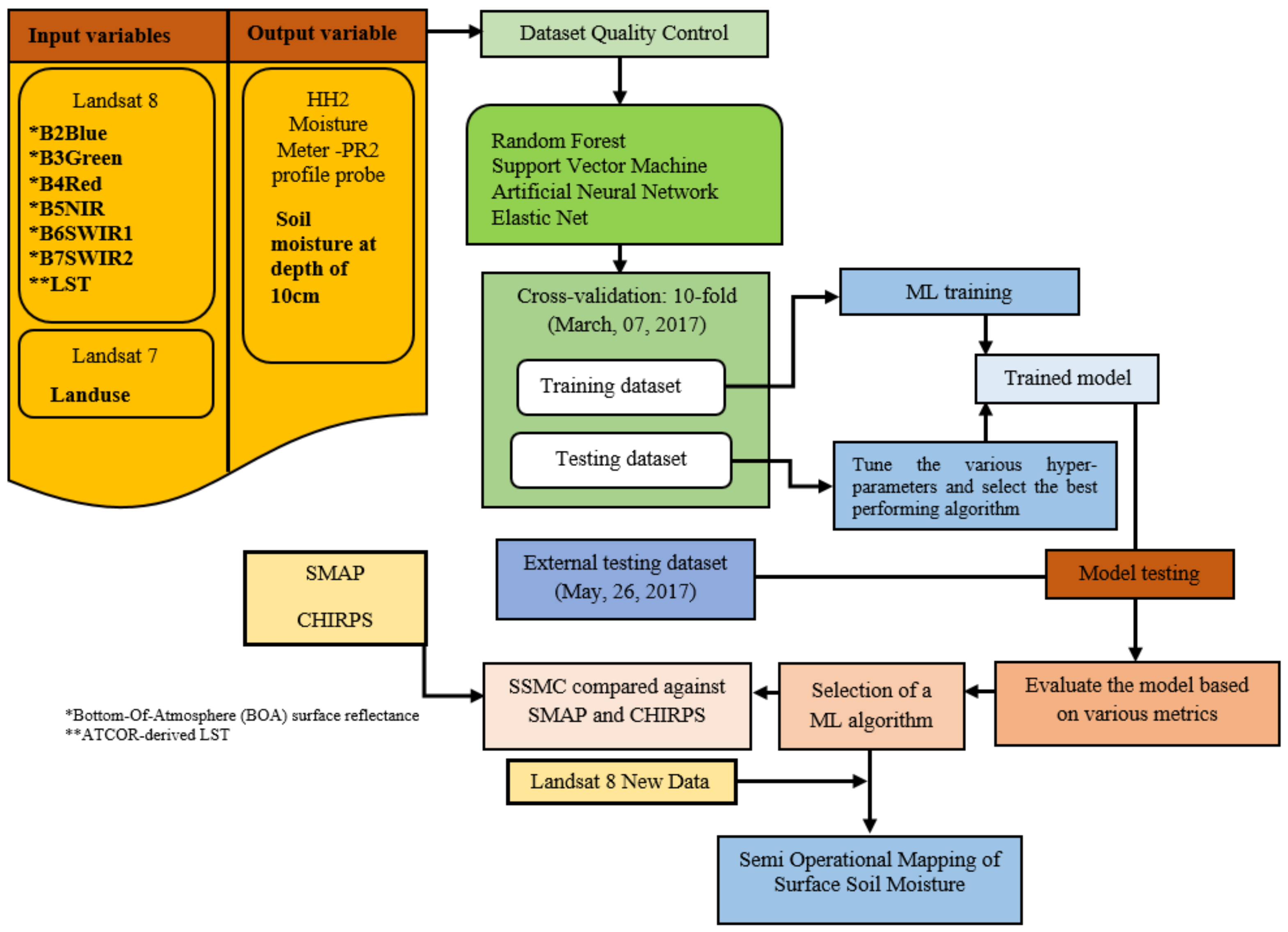
2.2.2. Landsat 8 Satellite Data

The Landsat 8 satellite consists of two sensors, the operational land imager (OLI) and thermal infrared sensor (TIRS) with the revisit time (at lower latitudes) of 16-days. Two satellite scenes from 7 March and 26 May 2017 were downloaded, and were georeferenced to the WGS84 datum, UTM projection Zone 40. The study area falls within the Worldwide Reference System (WRS) path = 160 and row = 35. Landsat data were obtained from the United States Geological Survey (USGS) Earth Resources Observation and Science (EROS) Center archive (http://earthexplorer.usgs.gov/). Originally, the distributed Level 1 TIR (Band 10 LWIR and Band 11 LWIR) data was already resampled from 100 m to 30 m resolution by cubic convolution resampling [49]. The spectral bands used in this study included MS bands (blue (0.45–0.51 μm), green (0.53–0.59 μm), red (0.64–0.67 μm), near-infrared (NIR; 0.85–0.88 μm), shortwave infrared 1 (SWIR 1; 1.57–1.65 μm), SWIR 2 (2.11–2.29 μm)), and thermal bands (LWIR1 (10.60–11.19), and LWIR2 (11.50–1251)).

Figure 2. Major soil reference groups and land-use classes of the study area and the location of the point samples on different land-use types. Precision separation of irrigated and rainfed areas might be under bias (For more details [50]).

Figure 2. Major soil reference groups and land-use classes of the study area and the location of the point samples on different land-use types. Precision separation of irrigated and rainfed areas might be under bias (For more details [50]).

2.3. CHIRPS and SMAP Datasets

For further analysis, Climate Hazards Group InfraRed Precipitation with Station data (CHIRPS) and Soil Moisture Active Passive (SMAP) satellite have been used to compare their agreement with the soil moisture derived from the present study. The CHIRPS quasi-global rainfall dataset systematically developed by the USGS in collaboration with the EROS center, have been distributed over the past decade by integrating satellite imageries and in situ gauge-collected observations at 0.05° spatial resolution [51]. NASA’s SMAP provides information about soil moisture contained in surface layers of the soil with a 9-km spatial resolution at a global extent by combining L-band passive (radiometer, 1.41 GHz) and active (radar, 1.26 GHz) microwave. Time series of precipitation and Level-3 (L3) surface soil moisture were used across the study area in 2017 and were obtained through the Google earth engine (GEE) online platform (https://earthengine.google.com/).

2.4. Pre-Processing of Data

Digital numbers (DNs) of the Landsat imagery were converted to surface reflectance using the ATmospheric CORrection (ATCOR3) model of PCI Geomatica 2018 software [52]. ATCOR is an add-on module of PCI Geomatica, which applies MODTRAN 4 RTM to generate look-up tables for different atmospheric input parameters. The visibility values for the image acquisition time were obtained from the Sabzevar Weather Station, and as Sabzevar locates in the continental areas with urban and industrial aerosol sources, an urban aerosol atmospheric model with mid-latitude winter and spring standard atmospheres were selected. The calibration files for Landsat 8 were retrieved from the image metadata file for the band-specific gain and bias values. Topographic correction is very important in the study area with rugged terrain. In this study, ATCOR-3 was applied for rugged terrain effects on Landsat 8 data acquired over the study area by incorporating ASTER DEM data and their derivatives such as aspect, slope, sky view factor, and cast shadow. DNs of the thermal infrared sensor were also corrected into surface temperature with ATCOR module. The ATCOR Surface Temperature workflow uses input thermal bands in scaled radiance (raw DN values), a DEM and terrain derivatives, and, optionally, thermal flux settings from Sabzevar Weather Station (e.g., elevation reference field, air temperature field, and water vapor partial pressure field, and air temperature gradient) to generate a surface temperature of the thermal image. The relationship between the fraction of green vegetation cover and SMC was analyzed through the croplands. The fraction of the vegetation classes were classified by SPEAR Tools, ENVI 5.3 on 7 March 2017. Normalized difference vegetation index (NDVI) usually applies for vegetation delineation, with values in the ranges from 0.05 (for sparse vegetation) to 0.7 (for dense vegetation cover) [53].

Geometric correction of satellite imagery was not performed on the data because level 1TP products are geometrically corrected using ground control points (GCPs) with less than a half-pixel circular error [54]. However, the Landsat 8 satellite images were geometrically double-checked by selecting control points (CPs) from well-defined locations such as crossovers of roads and other well-defined features from the Google Earth image. The total root mean square error (RMSE) of the registered Landsat 8 satellite images was 0.52 pixel.

2.5. Statistical Evaluation of the Input Data

Predictor variables were first statistically processed and screened to ensure their quality using XLSTAT software, Add in soft, New York, NY, USA before they were used to estimate SMC. The Grubbs test was used to identify the high level of presence of outliers among variables which may have a large impact on the model. Data normalizing has not been used in this study because the value range of predictor variables may not be the same due to intra-month fluctuations of remote sensing data. Normal distribution of the SMC data and predictor variables have been then checked by means of the jarque-bera (JB) test [55]. The JB statistic test compares the discrepancy between the distribution of data and an ideal Gaussian distribution [56]. To understand the statistical relationship of the eight predictor inputs on surface soil moisture, cumulative sums (CUSUM) statistic was used to measure the linearity and nonlinearity fashion. The CUSUM statistic measures the strength of linear association, which is defined as a running sum of the number of observations above and below the fitted regression line between dependent and independent variables. It is expected the points above and below the line are randomly scattered, when the relationship is linear and therefore the CUSUM statistic is small. One-way analysis of covariance (ANCOVA) is also used for assessing the influence of landuse as a categorical variable on SMC.

The presence of outliers data may give rise to a biased model [57] and a less accurate estimate of soil moisture. Therefore normal distribution test and outliers test of the variables have been checked by means of the jarque-bera test and Grubbs test (

Table 2. Descriptive statistics of variables and statistical tests used for SMC estimation.

Variables	Min	Max	Mean	Coefficient of Variation	Skewness (Pearson)	Kurtosis (Pearson)	Jarque-Bera Asymp. Sig	Grubbs Test Asymp. Sig
LST	11.9	19.6	14.9	0.13	0.53	−0.65	0.196 *	0.89 *
Blue	2.8	16.8	6.7	0.46	1.95	3.44	<0.0001	0.03
Green	5.0	25.0	10.3	0.44	1.97	3.38	<0.0001	0.04
Red	5.0	32.6	12.8	0.49	1.92	3.15	<0.0001	0.06 *
NIR	6.8	40.1	22.1	0.46	0.28	−1.45	0.083 *	1 *
SWIR1	9.1	39.8	19.1	0.39	1.33	1.39	<0.0001	0.23 *
SWIR2	7.2	37.4	15.6	0.47	1.74	2.50	<0.0001	0.1 *
Soil moisture (%)	0.0	30.5	11.0	0.72	0.66	−0.29	0.154 *	0.6 *

* The samples follow normal distribution and there are no notable outliers in the data (data is close to α = 0.05), as the computed p-value is greater than the significance level alpha = 0.05.

). As it turns out some variables do not conform to normal distribution (p > 0.05) but met the absence of outliers assumption (p > 0.05). This micro-variability would be considered acceptable for the desired level of soil moisture estimation that can be detected at the scale of sampling based on the current study. From a descriptive point of view, it can be stated that the data are sound without major biases and acceptable for machine learning modeling (Table 2). The range of coefficient of variation (CV) for soil moisture is 0.72, considerably high, representing that soil moisture in the datasets has a great level of dispersion around the average and therefore sampling points relatively covered a variety value of soil moisture content. Despite considerable variation in soil moisture among sites, the relative variability (i.e., CV) of spectral reflectance of bands across sites was relatively similar, with red band and SWIR2 showing the highest CV and LST the lowest. This provided some degree of confidence in the soil moisture estimation.

2.6. Database for Machine Learning Regressions

In this paper, we applied the most commonly used machine learning methods, including random forests (RF), artificial neural networks (ANN), support vector machines (SVM), and elastic net regression (EN). The output cell size of SMC predictors was again set to 30 × 30 m and the snap raster was realigned to the resampled to ensure cell alignment. The area grid was 1164 rows by 1523 columns (i.e., the total number is 1,255,859 cells with excluding no-data pixels in the Extent domain of study area). A total of 10,046,872 predictor cells were created and all layers were then subsequently converted to points, from which appropriate CSV format files were created and the spatial databases of each factor used in the Orange 3.24.1 open-source machine learning software (http://www.ailab.si/orange) [58] to run MLs, and later re-conversion to incorporate them into the GIS database. The estimation of soil moisture data for the study area was converted to a raster grid with 30 × 30 m cells for the study area. Due to the huge amount of predictor data that is generated by GIS software, Arc GIS 10.7, there was a need to automate the process. Figure 3 represented the flowchart of the methodological approach used in the present study. The flowchart consists of four main steps: (1) data preparation including input variable selection (VIS/NIR/and SWIR domain, land surface temperature and Landuse) and output variable (surface soil moisture), (2) data splitting in machine learning, (3) machine learning algorithms, and (4) statistical validation of SMC maps produced by the machine learning algorithms (see Figure 3). Details of each step are described in the following sections.

2.7. Machine Learning Regressions

2.7.1. Tuning Machine Learning Models

The next important stage in using MLs is the optimization of model itself. Tuning plays an important stage in the performance of MLs especially when the tuned model is going to use for semi operational mapping of surface soil moisture. Choosing appropriate hyper-parameters will result in high accuracy which may truly be translated as the success of the model. Each ML has a different setting of hyper-parameters that govern the learning model. However, it is unknown beforehand which values of the tuned parameters for the models are suitable for the SMC estimation. For that reason, to achieve a high prediction performance with the models, some parameters need to be tuned in the training process of the established model. Although k-fold cross-validation is the most suitable technique for training a successful ML, but the full advantage of accuracy cannot be taken by ML without tuning the model by specific external testing data. External testing data use in generalization which is the main point in tuning MLs model parameters. Because it tells us how well the learning model applies to specific data not used by the model. In the present study, the best model hyperparameters were chosen after making a judgment about several settings with expert intervention. In order to be able to assess the generalization capability of the MLs, 10-fold cross-validation of the model (49 samples), and external testing (9 samples) was applied to machine learning regressions (See Figure 1 for more details).

The MLs developed in this study were also evaluated on external testing that does not contain any pattern used in 10-fold cross-validation. The same data were used for 10-fold cross-validation and external testing of the MLs. The proposed model is first trained and validated with data in March 2017 and then tested on data from May 2017 to gain a confident estimate of the models’ performance. In this way, the prediction of SMC for unused point samples in May 2017 in the models can be analyzed. In other words, possible external testing helps us to sure the robustness of the final model in intra-and inter-season. Therefore, when modeling soil moisture, it is necessary to evaluate the accuracy of the model by external testing. In this study, 15% of the whole datasets being used for external testing the ML. The training subsets were used to train the machine learning regression (MLR), while the validation subsets to compute the cross-validation of the trained model. The validation subsets served as independent noise data to test the generalization capabilities of the trained MLR, especially when the training data are limited. The MLR was also compared by a k-fold cross-validation framework, sometimes called rotation estimation, as the heuristics technique [59]. The cross-validation estimator delivers nearly unbiased estimate information on model accuracy since the model is tested with k-folds not involved for model development [60]. The performance of the RF, ANN, SVM, and EN models on the full data set has been evaluated in this study by 10-fold cross-validation [61]. This cross-validation was applied to show that the experiment results of the algorithm are repeatable and not dependent on a particular subsample of the database. K-fold cross-validation includes randomly dividing the data into 10 k equal sized subsamples or folds. Iteratively, 8 subsets were applied to train the model, 1 as a validation dataset to stop the training procedure, and 1 as a test set to evaluate the performance of the model. This procedure has been repeated 10 times for each fold sequentially, which means each of the 10 subsets was applied once as a test set [62].

2.7.2. Artificial Neural Networks (ANNs)

A multi-layer perception (MLP) is a class of feedforward neural network (FNN) which has been selected to estimate surface soil moisture content. The configuration of the ANN has to be designed by the trial-and-error procedure because there are no definitive rules to find out the optimum configuration [63]. The following hyperparameter settings have been introduced: 6, 4, or 3 input neurons, 3 hidden layers, a regularization parameter of 8, and a maximum of 200 iterations. In this study, the identity activation function is used for all of the neurons in the hidden layer which is equal to fitting a linear regression model (note that an identity function is always employed as the activation function in the output layer). The backpropagation (BP) algorithm is a common gradient-based algorithm used for training FNNs. In order to solve some of BP problems, metaheuristic algorithms have been represented to train FNNs [64], namely the limited memory Broyden–Fletcher–Goldfarb–Shanno (L-BFGS) algorithm as the family of quasi-Newton, stochastic gradient descent (SGD), and Adam method [65]. The Broyden–Goldfarb–Shanno (BFGS) is used in this study, which is one of the promising methods for training neural networks and it is the best popular quasi-Newton algorithm [66] for general optimization as well as general machine learning [67]. BFGS method is not dominated by noise and has great advantages over the conventional backpropagation (BP) algorithm, including superlinear convergence, good approximation and generalization abilities, high accuracy, and less prone to overfitting [68,69,70]. Regularization used in this study which can use in filtering out noise from data, and eventually avoid overfitting by adding bias to penalize extreme parameter weights [71].

2.7.3. Support Vector Machines (SVM)

SVMs are a class of supervised learning algorithms, which is derived from statistical learning theory and were first introduced by Vapnik [72]. In some ways, SVMs are closely associated with ANNs [73]. The SVMs have been successfully applied for both classification and regression proposes [73,74]. SVM uses a kernel function for transforming the input data and then apply linear regression to the transformed data [75]. SVM involves two steps, including, (1) selecting an appropriate kernel type and setting kernel parameter (kernel width G) and (2) specifying the penalty parameter C [76]. A set of varying hyperparameters, with the best results obtained with regression cost (C) of 0.5, complexity bound (V) of 1.00, sigmoid kernel with g 0.98, c 0.10, numerical tolerance of 0.03, and a limited value of iterations, equal to 200, have been selected.

2.7.4. Elastic Net Regression (EN)

Regularized regression techniques were developed to overcome the weaknesses of ordinary least squares method regression [77]. In such a method, a penalty parameter, representing a bias to be added to the regression coefficients in the equation, is introduced as a regularization parameter [78]. The significance of imposing the penalty is to shrink the coefficient values towards zero or near zero which effectively allows less independent variables to have a coefficient close to zero or equal zero [78]. A linear regression model that applies the L1 regularization technique is called Lasso (least absolute shrinkage and selection operator) and a model that uses L2 is called ridge. Elastic net regression can improve the predictive performance of Lasso regression by combining the grouping effect of ridge regression with the lasso regression. Thus, elastic net has two tuning parameters: α controlling the balance between L1 (lasso) and L2 (ridge) penalties, and λ controlling overall strength of the penalty [78]. The elastic net regression adopted in this study with the hyper parameter settings: α = 0.15 and L1:L2 ratio of 0.71:0.29. These tuning parameters were obtained using both k-fold cross-validation and external testing data set.

2.7.5. Random Forest (RF)

RF is a nonparametric method that is robust to noise in predictors and thus does not require a preselection of variables [79,80]. RF has several main advantages over another statistical modeling, such as the ability to find high dimensional non-linear relationships, using of categorical and continuous predictors, resistance to overfitting, and relative robustness to noise in predictors and therefore does not need a preselection of variables, and only a few user-defined parameters [80,81]. Numerous trees are composed by the algorithm and the final predictions involve the average of the results from all developed trees in the forest [82]. It is necessary to define a priori three user-defined parameters before running the model, namely the number of trees in the forest, the number of attributes for consideration at each split, and growth control which represents the depth of individual trees and split subsets. Applying RF the following hyperparameters have to be set: number of trees, number of random attributed at each split, the seed for random generator, and depth limit of individual trees. They have been set equal to 50, 5, 5, and 30, respectively; furthermore, limit the depth of individual trees (pruning) has been adopted to avoid over-fitting.

2.8. Model Validation and Assessment

Model validation deals in this study with regression metrics and statistical tests. In order to assess the performance of the developed models quantitatively, evaluation metrics involving the mean bias error (MBE), mean absolute error (MAE), root mean square error (RMSE), index of agreement (D-index), and Nash–Sutcliffe model efficiency coefficient (NSE) have been used. MBE is primarily used to indicate the average bias in the model. The positive MBE indicates an overestimation in the predicted SMC while a negative MBE shows an underestimation [83]. The MAE is the simplest measure of estimate accuracy which measures the average magnitude of the errors in prediction data, without considering their direction. It is the absolute value of the difference between the predicted values and the observed ones. MAE may be preferred because it is a simple error metric and is less sensitive to outliers than RMSE [83,84]. RMSE measures the variation between predicted values by a model and the measured values. The lower RMSE indicates good agreement between estimation data and observation data. Both MAE and RMSE represent average model prediction error from 0 to ∞ in the same units as the response variable.

The Nash–Sutcliffe efficiency (NSE) and index of agreement (D-index) coefficients as normalized error-index statistic have been used in this study to seek the model on the basis of its reliability. D-index was proposed by [85] as a standardized measure of the degree of model prediction error which is dimensionless and in the range of 0–1. The index of agreement does not measure correlation or association between two series of variables. Instead, it provides a measure of the agreement to which the model predictions match exactly the observed data with no proportionality [86]. However, it is very sensitive to extreme values due to the squared differences. Nash and Sutcliffe [87] proposed an alternative goodness-of-fit index to overcome the limitations of the correlation coefficient, which is referred to as the efficiency index (NSE). NSE represents the relative magnitude of the residual variance compared to the measured data variance. The NSE theoretically varies on the range −∞ to 1 and higher values of NSE show a better agreement between predicted values and observations, a model with NSE of 0.0 is no more accurate than predicting the mean value, and negative values represent that the model is worse than the mean value as a predictor. Model performance is considered “acceptable” when NSE ≥0.50, and D ≥0.70 [88]. Once the highest accuracy model according to evaluation metrics on the validation data has been identified, another field test data has been selected to evaluate the model performance; this procedure has been set up to check the accuracy of SMC prediction with the same model. The model has been then finalized to make SMC predictions for the entire extent of the study area and thus generate a map of the predicted soil moisture.

3. Results

3.1. Linearity Test between Soil Moisture and Optical Domain

The statistical comparison between single bands and SMC shows that the reflectance in visible wavelengths decreases as moisture content in areas (

Table 3. CUSUM statistic and Correlation (Pearson) among the wavelength reflectance, land. Surface temperature and soil moisture content from total measured data.

Variables	CUSUM Statistic p-Value	Pearson Correlation
LST	0.7334	−0.267
Blue	0.8547	−0.370
Green	0.0006 *	−0.231
Red	0.0006 *	−0.257
NIR	0.0064 *	0.346
SWIR1	<0.0001 *	0.028
SWIR2	<0.0001 *	−0.096

* Nonlinear is significant at a level of 0.05.

). There is also a tendency that wetter soils correlate to lower temperatures. The results for the (SWIR) spectral regions show no clear tendencies. The test for non-linear correlations indicates that only the blue band and surface temperature are linearly correlated to SMC. These suggest that spectral surface reflectance of the samples over different wavelength is influenced by surface soil moisture in non-linear form during the wet and cold season. It becomes clear from Table 3 that there is an effective absorption for wet soils in the visible domain. In contrast, it is found that the correlation between NIR and soil moisture is positive (also given in Table 3). The results of the ANCOVA show a significant relationship between landuse and SMC (p < 0.05). Forested areas (5–25%) have the highest SMC (20%) and Irrigated cultivated areas and Forested areas (Less than 1%) have the least SMC (7%). Higher soil moisture in the Forested areas (5–25%) may be due to relatively low potential evaporation from the soil surface. Haplic Fluvisols (Calcaric) exhibits high soil moisture values with an average of 30% moisture content. These soils are characterized by young alluvial soils mainly found along rivers or other low terrain positions, which show stratification or other evidence of recent sedimentation. aplic Fluvisols (Calcaric) are located in more humid areas in the study area because they receive runoff water additional to their portion of precipitation. The lowest value of moisture content (less than 10%) was found in Haplic Calcisols which is characterized by soils of (semi-) arid regions with enrichment of secondary carbonates.

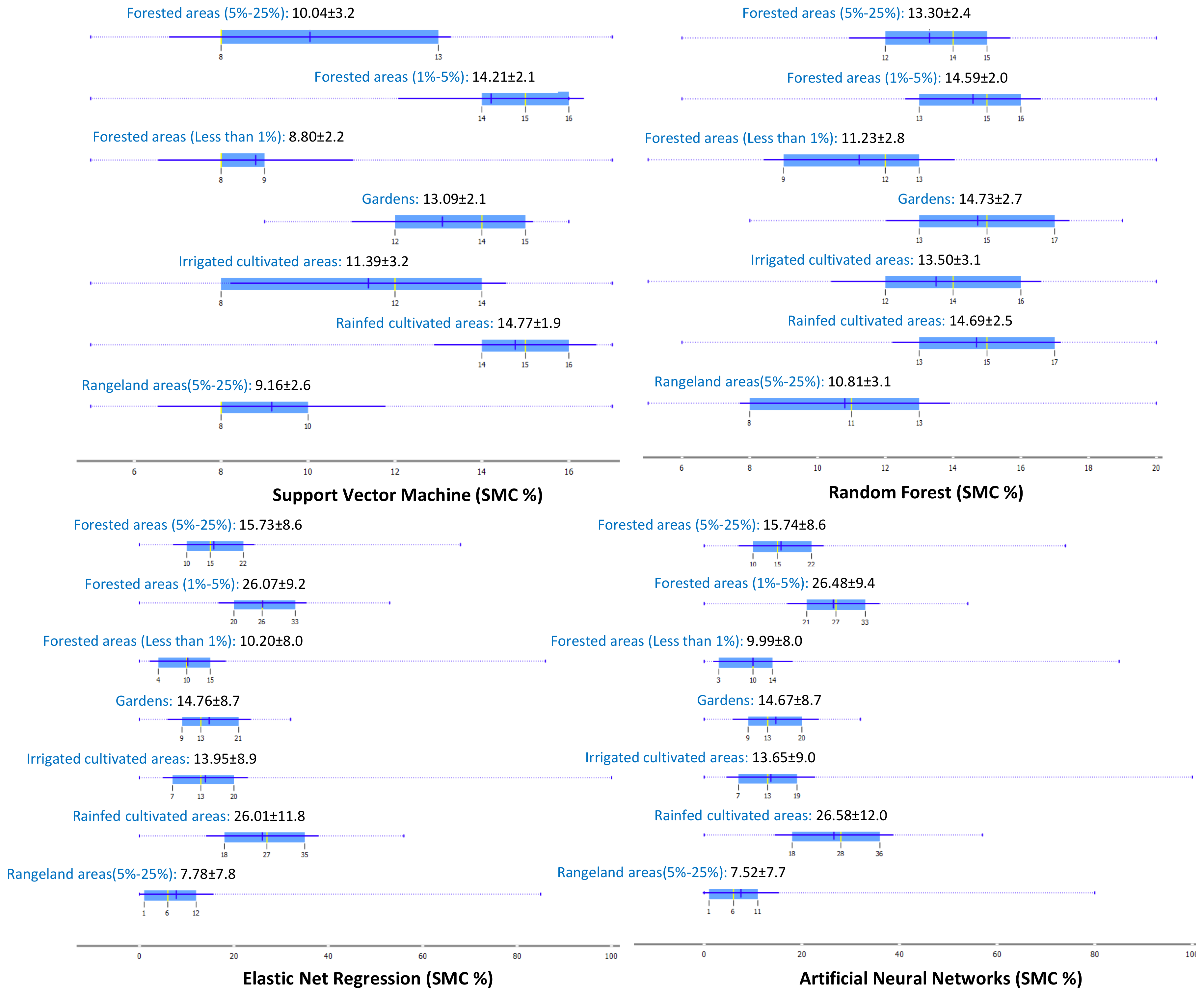
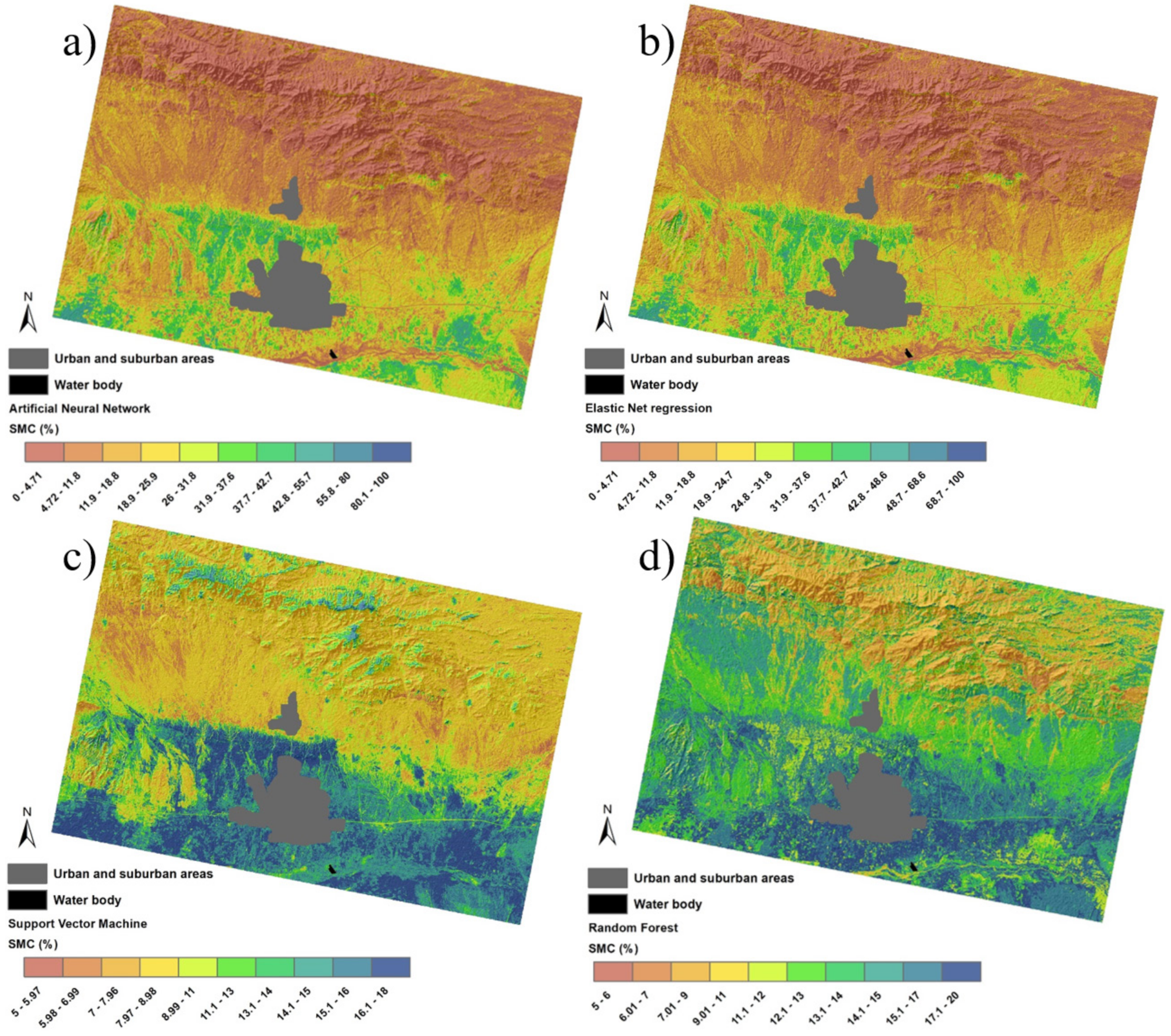
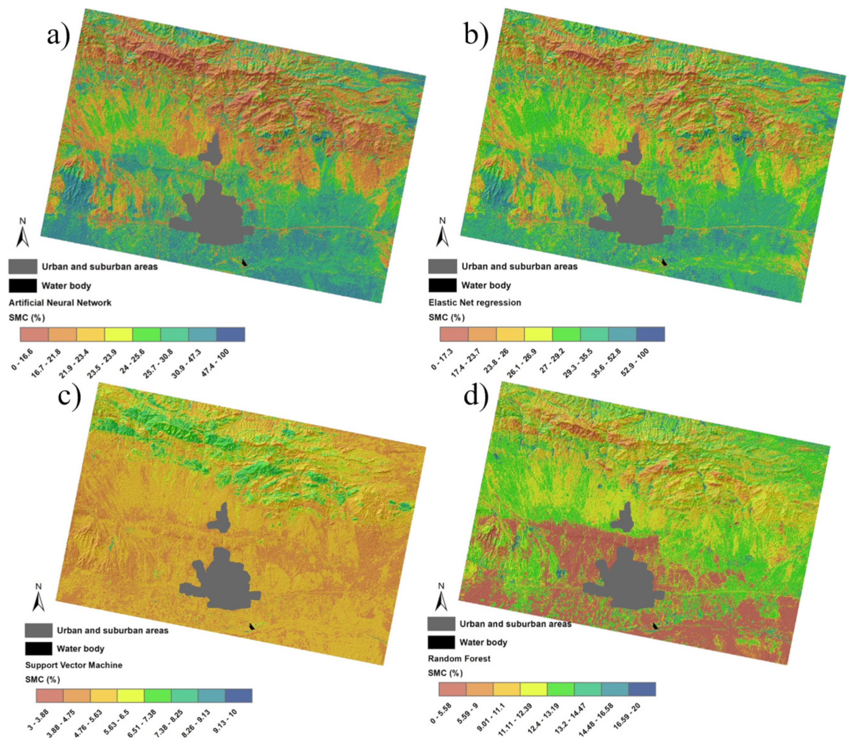
3.2. Estimating Soil Moisture by Implementing Machine Learning Models

The soil moisture information provided by the MLs is used to produce a box plot in conjunction with Landuse classification map (Figure 4). It can be seen that there are some distinct differences between the land-use classes in terms of soil moisture. Visual inspection of box plots showed that there was generally the same SMC prediction between EN and ANN from entire landuse classes. The mean comparison of EN against ANN showed that these techniques gave the same range of soil moisture prediction for the Landuse classes. The box plots also represented RF having a slight edge over SVM. Box plots indicate that forested area (less than 5%) and rangelands (5–25%) have the lowest mean of soil moisture and slightly different from the other land-uses. The entire standard deviation of the mean soil moisture clearly discriminates RF and SVM from the EN and ANN (blue highlighted area in Figure 4). Values of the first (25%) and the third (75%) quantiles of soil moisture for EN and ANN have the same values for the eight land-use classes, while the entire range of SMC values (from the lowest to the highest value in the data set for the soil moisture) is not notable. The boxplot of SMC in Figure 4 shows that the rainfed cultivated areas and forested area (1–5%) tend to be more SMC than the other land-use classes. The standard deviation of the mean of the SMC derived from ANN and Elastic Net regression models are broader, indicating very high variations of SMC in terms of soil moisture estimation (thin blue line in Figure 4). However, the standard deviation of the mean for SVM and RF is distributed narrow, presenting more pixel values in the low range of SMC which indicates a low variation of soil moisture. Overall, the ratio of the variance to the mean represents that both RF and SVM generally estimate SMC with less dispersion with values of 0.25 and 0.32 across all categories. In contrast, the dispersion values for ANN and elastic net regression models are 0.78 and 0.76, respectively.

After implementing models, ANN, SVM, RF, and EN regression have predicted soil moisture content of the study area showing the spatial distribution of soil moisture at 30 m resolution. The models have been applied to the landuse data and the Landsat 8 OLI and TIRS data on image dated 7 March 2017, that captured the entire study area to map soil moisture content (Figure 5). Relatively high SMC were found in slope with a gentle gradient in the lower parts of South of the area and near to the agricultural and urban and suburban areas and also coalescing alluvial fans connecting to the mountain, however, mountain lands in North of the area experienced very low SMC (less than 6%), dominated by less foliage with rock exposure, and steep slope in this area. The results show that the spatial pattern of dry and wet trends is mostly the same but the range of values is slightly different. Almost all the models have totally agreed upon the low SMC to find the high land area and highest levels of SMC on areas of river floodplains and alluvial fans on 7 March 2017; this behavior has been mainly shown by ANN and elastic net regression model. The SMC map of ANN and Elastic Net regression (Figure 5) is too small to show a few soil moisture saturated individual grid cells. These cells of wet areas show a close correspondence with the local poorly drained areas in the study area. This is due to local control of terrain which has an influence on the wet pattern of soil moisture where areas of high local convergence may be the cause of a temporary increase of water content following rainfall in the soil.

The obtained models have been iterated to estimate SMC at the next time step on 26 May 2017, as testing data sets (Figure 6). Analyzing the results during testing, it can be observed that ANN and Elastic Net regression models have represented very wet conditions compared to SVM and RF which can be seen for training data sets as well. For SMC testing dataset the ANN and Elastic Net regression models have estimated the SMC of 0–100% while the SVM and RF models estimated the SMC of 3–10% and 0–20%, respectively. This spatial variability could be due to both model structure and data noise. Therefore, even for the same data sets, different models may have different implications for the model fit to the data and will perform poorly in generalization.

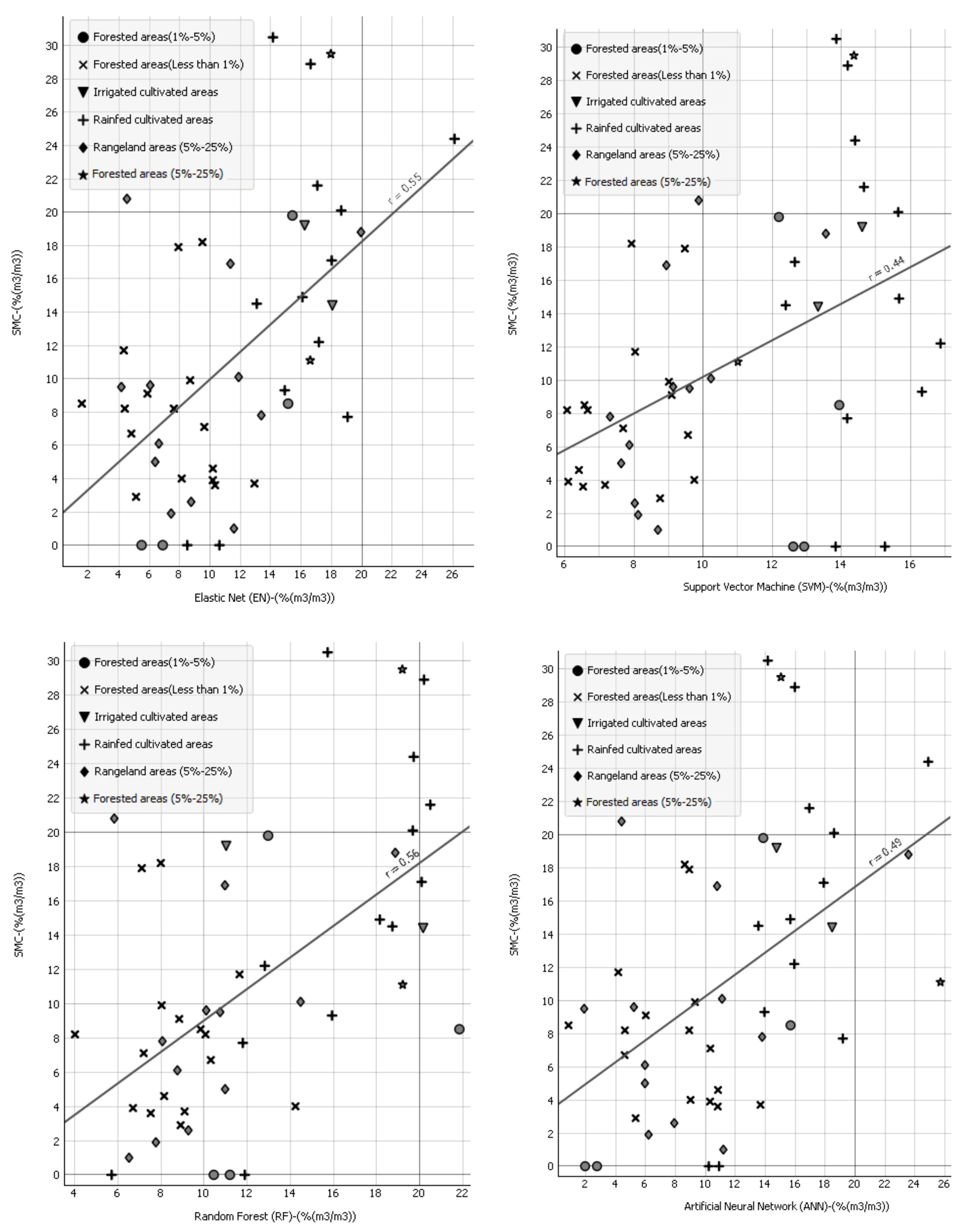
3.3. Validation of Machine Learning Models

A comparison between the results from the testing data set (

Table 4. Prediction error metrics of the ANN, SVM, RF, and Elastic Net regression. 7 March 2017 10-fold cross-validation dataset, and 26 May 2017 external testing datasets.

Methods	MBE		MAE		RMSE		d		NS
	March	May	March	May	March	May	March	May	March	May
SVM	0.25	3.19	5.51	7.28	7.20	8.56	0.46	0.31	0.19	0.06
ANN	−0.20	−15.0	5.85	15.08	7.27	16.5	0.63	0.52	0.17	−2.46
RF	−0.90	2.16	5.0	3.46	6.25	4.60	0.72	0.91	0.39	0.73
EN	−0.30	−18.7	5.55	18.7	6.76	19.7	0.67	0.44	0.28	−3.94

) shows that the estimated SMC for RF model has a RMSE of 4.60%, Nash-Sutcliffe efficiency 0.73, an index of agreement 0.91, and a smaller bias (MBE = 2.16) compared to other ML models. The RF model consistently outperforms all other models. Values from the RF model are acceptable comparing to those from the other three models for testing datasets; therefore, it has been chosen as the best method to predict SMC at the unsampled locations in this study. Visual analysis of SMC has shown that RF can be considered a robust spatial predictor model that could estimate SMC in different topographic features and slope and aspect topography (Figure 5). The results show that there are large differences in error rates among the four data mining techniques. There are also relatively big spatial differences in SMC among the four techniques, specifically, the spatial differences of SVM and RF are thoroughly obvious. Furthermore, the correlation of models increased when landuse included in MLs (ANN = 0.49, SVM = 0.44, RF = 0.56, and Elastic Net regression = 0.55) compared to that obtained without integration landuse data (ANN = 0.48, SVM = 0.4, RF = 0.5, and Elastic Net regression = 0.5), which has suggested that auxiliary geospatial data produced better SMC prediction than was expected using the optical values alone.

The scatter plots between observed and retrieved soil moisture covered by six dominant land-use types using ML models are shown in Figure 7. According to the scatter plots, SMC could be predicted with moderate accuracy for the RF (r = 0.56), while the SVM had the lowest accuracy of estimation.

4. Discussion

4.1. Correlation of Soil Moisture and Predictor Variables

Nonlinearity between soil moisture content and spectral reflectance in topsoil was significantly observed over the Green, Red, NIR, SWIR1, and SWIR2 wavelength, and linearity observed for Blue wavelength and LST. Soil spectral reflectance decreases at 0.4 µm to 1 µm wavelengths when moisture content increases [89]. An earlier study has shown that the decrease of spectral reflectance upon wetting of soil is non-linear because of the hydraulic behavior of water in unsaturated sand [90]. Soil reflectance was observed to be nonlinearly correlated with soil moisture, which was well correlated by a curvilinear exponential model between the 1100 and 2500 nm wavelengths [91]. Even though green and red wavelengths have a nonlinear relationship with SMC, the Pearson correlation coefficient represents a fairly weak negative relationship of visible wavelength with SSM [23,92]. SSM experiences a fairly weak positive relationship with NIR wavelength (Table 3) and this trend is consistent with the results of other studies that used reflectance of MODIS data in a tropical area [92]. This is likely the result of [27] that found the positive correlation between NIR wavelength and SMC for bare soil area and negative correlation with vegetated soil, however, the existing studies showed an exponential negative relationship between soil moisture and NIR reflectance [23]. Estimating surface soil moisture is more complicated over NIR reflectance for a mixture of bare soil and vegetation because the relationship between NIR reflectance and moisture measured in the field for vegetation and bare soil is totally different [27]. The NIR reflectance of vegetation is higher than that of bare soil [93]. These differences results were coming from different examined soil samples which collected from miscellaneous landuse characteristics. Nagy et al. [26] found that the increase of soil moisture content did not result in linear changes in reflectance value at 950 nm and 450 nm and the equations for SMC estimation were set up separately for different soil texture. The linear correlations between spectral features and SMC over 25–30% and less than 5% of moisture content is not significant [26].

In this study, Pearson’s coefficient did not capture the linear correlation between SWIR1 and SWIR2 wavelength and SMC. However, the best correlation between reflectance and SMC was found for the reflectance of short-wave infrared bands SWIR1 and SWIR2 for bare soil and vegetated soil [27]. It has been shown that soil spectral reflectivity is recognized as a function of water content but spectral reflectivity can be affected by intrinsic soil factors such as the amount of organic matter, particle size distribution, mineral composition, surface roughness, and color of soil elements [94,95]. Land surface temperature shows to have a week negative influence over soil moisture (Table 3) which highlighted the more complex behavior of the SSM-LST relationship due to the complexity of land surface and for a mixture of bare soil and vegetation [94,96,97].

The results of the study show a significant relationship between landuse and SMC (p < 0.05). Land-use is very significant in determining the spatial variability of SMC because it influences vegetation cover and infiltration and runoff rates, evapotranspiration processes, soil surface characteristics [98,99]. Landuse can even eliminate the effects of related parameters of the topography on SMC [100]. Several studies provide solutions for estimating soil moisture by reflectance images and auxiliary geospatial data [101,102]. Higher soil moisture in the Forests of Haloxylon spp (5–25%) may be due to relatively low potential evaporation from the soil surface. It was observed in a previous study that the amount of clay and silt increases rapidly when sand dunes are stabilized by Haloxylon spp because of suspended particle accumulation and fine particulates which are produced by the weathering mechanism of sand [103]. Increasing clay and silt content also had a slightly positive correlation with soil water content [104]. Topsoil (0–5 cm) moisture content in the youngest Haloxylon ammodendron was significantly less than older plantations [104] because soil surface experiences high evaporation potential due to high solar radiation.

4.2. Perspective of Machine Learning Algorithms in Soil Moisture Content

Soil moisture retrievals were computed using four different machine learning algorithms in a semi-arid area, using optical and ancillary data at high spatial resolution. Based on the performance indices reported in Table 4, it is noted that the RF model estimated soil moisture has RMSE less than 4 for all the selected samples during the testing phase. These comparative results are consistent with those of [105] who used VNIR hyperspectral imaging over the plot set up with an area of one square meter and the results indicated that RF outperformed SVR, ANN, and EN in estimating SMC. Although the other studies reported slightly better estimation accuracy [106] of SVM, this may be due to the different scales of the study areas, topography conditions, soil characteristics, sampling densities, incorporating the missing environmental data or quantity and quality of the auxiliary data used to estimate SMC [107,108]. It was indicated that the uncertainty of SMC does not vary with the spacing of point samples in southeastern Australia [109], however, it was represented that uncertainty decreases as the sampling density increased in the Australian National Airborne Field Experiments 2005 (NAFE’05) [107]. From these studies, it can be concluded that the performance of models to estimate SMC is very site-specific and the complex characteristics of uncertainty and the sampling configuration are very dependable on the study scheme. Although the accuracy of the capacitance probe for field soil moisture measurement is still under investigation, the integration of PR2 Profile probe with remote sensing data is capable of monitoring surface soil water content especially when the amount of surface soil water is required on a site-specific [110]. Since a universal relationship between SMC and remote sensing data does not exist, it must be explored empirically by calibration data.

It can be obviously seen in previous researches that ANN model and SVM model have been the most popular method to predict the soil moisture content due to solving non-linear relation between input and output with high accuracy [28]. However, the present study showed that the predictive results of ANN and SVM on the testing dataset are vulnerable which is affected by the uncertainties on nonlinear relation. ANN and SVM structure with the best performance is difficult to be determined [111] however RF is fast to train and tune as compared to other ML methods [112] because RF only has a few tuning parameters. In the present study, we found larger spatial differences in some cases among the machine-learning algorithms. EN offers the most comfortable usage technique because very few parameters have to be optimized and calculation times are marginal for big data such as remote sensing data. However, these advantages are covered by poor prediction performance. Random Forest in contrast is easy to use since only two parameters need to be set by the user. It was noted that RF model is suitable when sample plots and variation are relatively large (i.e., LAI with more than one growth period) [113]. As shown in this study, surface soil moisture was measured in the fields in two periods with high variation. An important characteristic of RF is that it is relatively resistant to overfitting problems [114] and the RF algorithm has well proven to handle high-dimensional data sets and, thus, has a high tolerance for data faults [115]. However, it may be difficult to find an efficient train RF model with a small sample size [116]. The learning of ANN is based on large samples and the performance of the ANN is affected by the complexities of the network structure and the sample. The higher learning accuracy by increasing more neurons may lead to weaker generalization ability. Therefore ANN makes prone to over-learning and reducing the ability for generalization [113] as it was shown for the testing dataset in this study (Table 4). The ANN model is more suitable when sample plots and variations are relatively low (i.e., LAI for a single growth period) [113]. Based on our results, the SVM model is the second appropriate for soil surface moisture estimations. At some point, a small sample size might be not enough for optimal training of SVM [113].

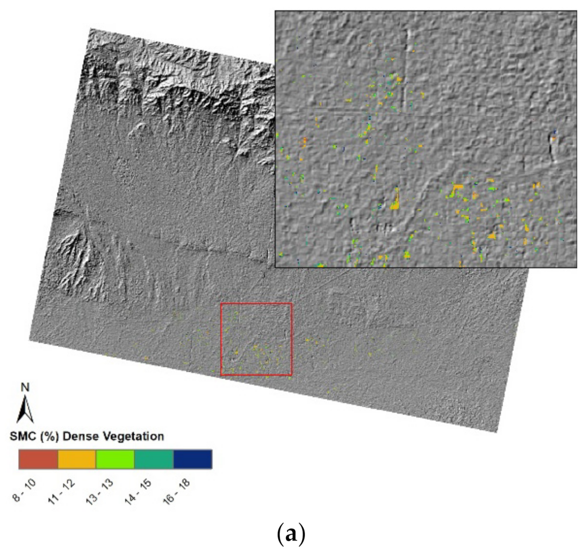
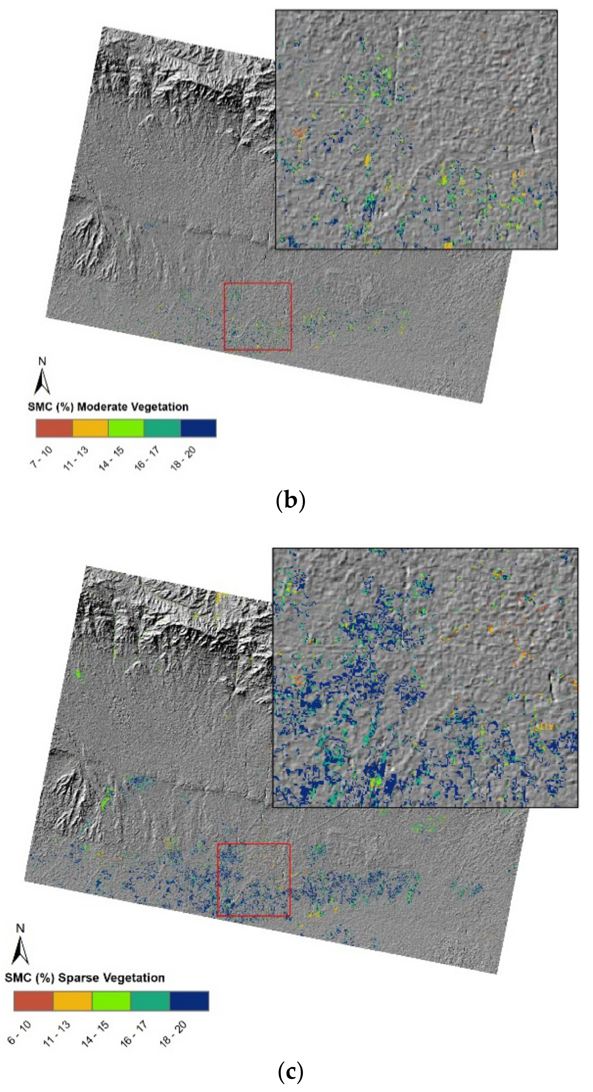
4.3. Soil Moisture Status over Croplands

SMC is thought to be controlled by soil texture, vegetation type, and microclimate. Figure 8 represents the soil moisture within three vegetation vigor classes (Dense, Moderate, and Sparse). As shown in Figure 8, the soil moisture has not a clear association with three vegetation vigor classes. Because the vegetation status (e.g., type, age, growth stage, and frequencies and durations of irrigation and leaf area index) are not uniform among different fields. Relative high soil moisture was observed for some croplands with sparse vegetation. This soil moisture status is clearest in Figure 8 where the croplands might be under a heavy irrigation event at the time the Landsat data was acquired on 7 March 2017. However, some parts of cropland with moderate to dense vegetation were experienced low soil moisture. In a general concept, high correlations were found in densely vegetated areas (normalized difference vegetation index) and SMC [117], however from Figure 8, this study represented that heavily vegetated areas do not always have a high amount of SMC. This finding is generally consistent with the results of Tianjiao, et al. [118], who noticed that different physiological characteristics of vegetation types have different effects on soil moisture content in a semiarid climatic zone. Dense vegetation also reduced the stability of soil moisture [119] that can be seen in dense vegetation areas in Figure 8. Also, some of the field areas in the study area were not irrigated during the growing cycle and were expected to be less moist. Cropland areas in the study area are dominated by expensive crops (e.g., Pistachios) and the relative soil moisture values of dense vegetation areas were generally less than 10%. Therefore water stress can influence heavily vegetated covers in the area over the study period. Different crop types have different water demands and respond differently to water stress that causes heterogeneity of surface soil moisture after uniform irrigation [29]. This soil moisture spatial heterogeneity for dense vegetation appeared in the form of cropping patterns. Vegetation influences soil moisture and researchers have found that different plant species can influence the spatial and temporal properties of the soil water content [118,120,121]. These studies clarified that plant species can consume amounts of soil water and cause soil drying [119,122,123]. Other factors such as soil texture, surface roughness, and the temperature of the upper soil layer affect soil moisture on the upper 5 cm of the soil [124]. Topographic variability, which influences soil properties and exposure to wind and solar radiation [125]. Therefore the global function of SMC index maps obtained on the different areas is not necessarily useful because they are extracted from a different environment, and calculated by various parameters. This issue complicates the monitoring of the SMC in a specific site.

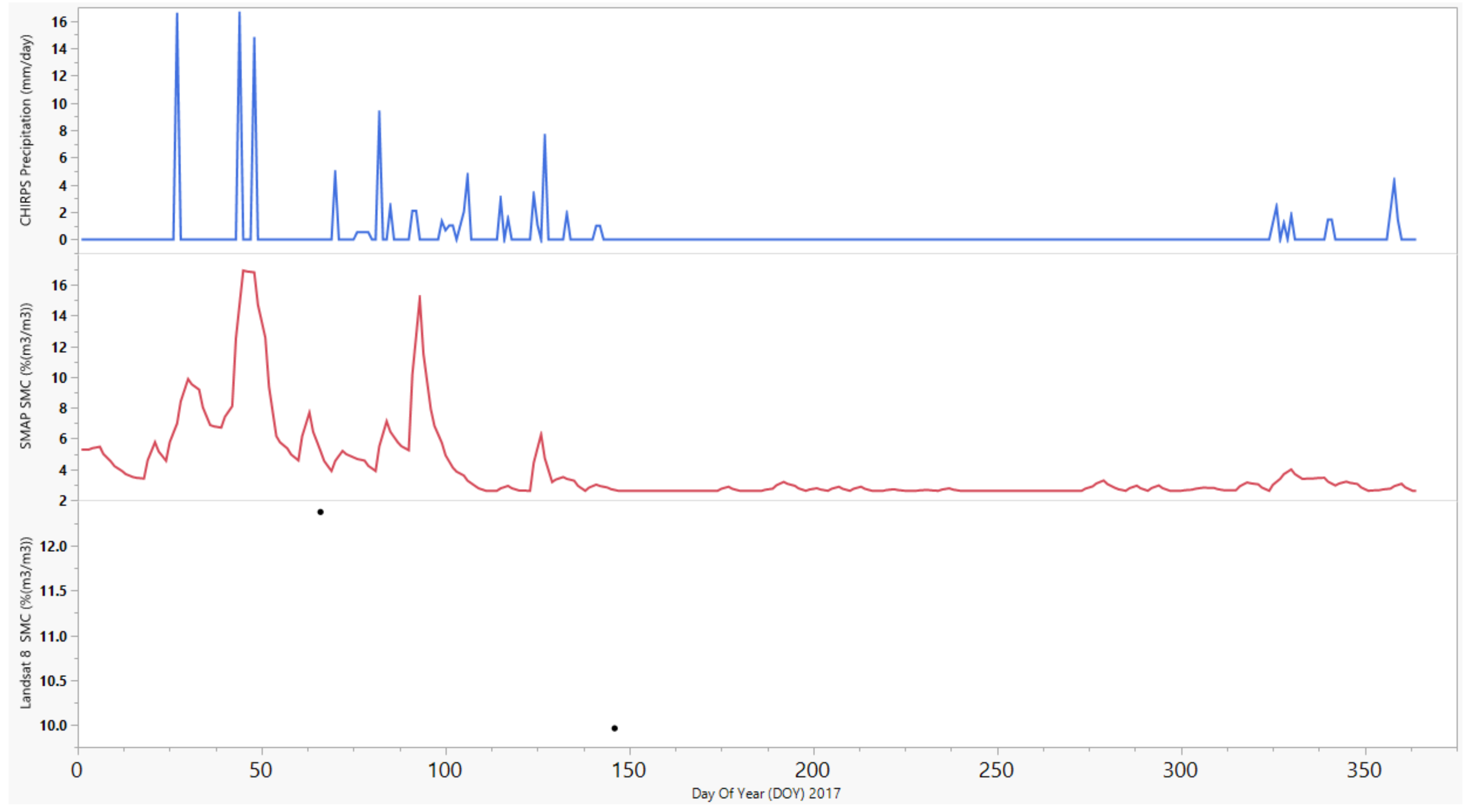
4.4. Further Analysis of SMC with Operational Satellite-Derived Precipitation and Soil Moisture Products

In this study, soil moisture estimates of the Landsat 8 from 7 March 2017 and 26 May 2017 were compared with the SMAP 9-km soil moisture product. Even though the coarser-resolution soil moisture estimates from SMAP cannot be used for pixel to pixel comparison, but the dry-down and wetting trends can be assessed for validating the algorithm. Therefore an average for the entire pixel of soil moisture estimation from landsat was used to compare with SMAP. However, an incorrect consistency of spatial resolution may have been introduced biases into the results. The CHIRPS gridded precipitation dataset with 0.05° spatial resolution were also used in order to facilitate the analysis of the SMC generated maps because precipitation is a proxy for soil moisture. Figure 9 represents daily precipitation data created by CHIRPS for the study area and particularly L3 SMAP products were also added to the time-series for evaluating the ability of the Landsat 8 SMC estimates in capturing the surface soil moisture due to precipitation. Figure 9 clearly indicates that the Landsat 8 SMC estimates at two days (black dot points) follow the precipitation events (e.g., wetting events at the beginning and dry downs at the end of the year).

The beginning of the wet season recorded accumulated precipitation of about 47 mm, since the ending of February, soil moisture trend for both SMAP and Landsat 8 derived soil moisture has started to increase compared to a dry season to less than 5% at the end of May. The effects worsened during the dry season with a rainfall deficit continuing to decrease soil moisture until the end of the season with about 0%. The corresponding L3 SMAP and Landsat 8 soil moisture estimates are slightly different. However, both soil moisture products exhibit a similar trend when the surface soil is mostly wet and dry. It is possible that some agricultural lands become wet from irrigation in the study area, despite there being no significant rainfall event.

Using satellite-based soil moisture estimates in arid and semi-arid areas has several advantages: (1) Regional coverage enables soil moisture monitoring of large part of natural ecosystems; (2) 16-day time period improves the ability to monitor the drought-related events in seasonal coverage; (3) precise measurement of water consumption for irrigation needs the soil moisture mapping in irrigated and non-irrigated areas; (4) the application of algorithms enables us to apply it for up-scaling SMC to other sensors with high temporal resolution and to capture the irrigation pattern. It must be stressed that this study used only two months (March–May 2017) and soil moisture estimates that can have higher uncertainties over regions of dense vegetation, and therefore validation procedure needs to be performed using in situ observations [126]. Therefore, care should be taken in generalizing results from the present study.

5. Conclusions

In this study, four different types of rapid nonlinear data-driven models (SVM, ANN, EN, and RF) for predicting the near-surface (5 cm) soil moisture (SMC) were established in practice over different land-use types by combining Landsat-8 surface reflectance data and land-use auxiliary geospatial data on a (30 m resolution) pixel basis. Predictions show good agreement with observed soil moisture measurements. Results from the RF, SVR, ANN, and EN modeling are compared with measurements obtained from PR2 field data and show that RF model performed better for soil moisture forecasting than the other three methods in testing cases. From the result of Nash–Sutcliffe efficiency, the predictive SMC produced from RF has the highest explanatory ability (NS = 0.73). The accuracy of machine learning methods depends on the selection of an appropriate function and parameters. Various techniques are often based on the vegetation index, triangle method, and trapezoid method in the optical domain to estimate SMC rather than on the reflectance of soils. It is represented in this study that deriving surface soil moisture from remote sensing data is still complicated, as the surface soil moisture is not just a function of the reflectance of soil, but is affected by spatial auxiliary data such as land-use types. This hinders solutions for estimating soil moisture using reflectance images. Clearly, the 30 m remotely sensed images show more spatial detail in the surface soil moisture quantitative estimates and also spatial pattern than the sparse ground measurements. This 30 m soil moisture can serve a variety of water resource applications such as watershed modeling over semi-arid climate. More detailed estimations of surface soil moisture will in turn benefit agriculture, with the monitoring of vegetation stress, and provide a valuable dataset for drought monitoring in a semi-arid climate. The limitations faced by this study were time, space, and amount of field soil moisture measurements. However, this study covers several gaps related to the usage of surface reflectance and land-use data, even if the potential of incorporating other variables for estimating soil moisture for future research is still excessive. In conclusion, the high-resolution gridded soil moisture presented in this study can be used in spatial decision support tools for precise irrigation scheduling and to indicate areas with plant potential limited by the lack of soil moisture.

References

1. Kim, S.; Liu, Y.; Johnson, F.; Sharma, A. A temporal correlation based approach for spatial disaggregation of remotely sensed soil moisture. In Proceedings of the AGU Fall Meeting Abstracts, San Francisco, CA, USA, 12–16 December 2016. [Google Scholar]
2. Keesstra, S.D.; Bouma, J.; Wallinga, J.; Tittonell, P.; Smith, P.; Cerdà, A.; Montanarella, L.; Quinton, J.N.; Pachepsky, Y.; van der Putten, W.H.; et al. The significance of soils and soil science towards realization of the United Nations Sustainable Development Goals. SOIL 2016, 2, 111–128. [Google Scholar] [CrossRef] [Green Version]
3. Keesstra, S.; Mol, G.; De Leeuw, J.; Okx, J.; Molenaar, C.; De Cleen, M.; Visser, S. Soil-Related Sustainable Development Goals: Four Concepts to Make Land Degradation Neutrality and Restoration Work. Land 2018, 7, 133. [Google Scholar] [CrossRef] [Green Version]
4. Kelley, C.P.; Mohtadi, S.; Cane, M.A.; Seager, R.; Kushnir, Y. Climate change in the Fertile Crescent and implications of the recent Syrian drought. Proc. Natl. Acad. Sci. USA 2015, 112, 3241–3246. [Google Scholar] [CrossRef] [PubMed] [Green Version]
5. Zareie, A.; Amin, M.S.R.; Amador-Jiménez, L.E. Thornthwaite moisture index modeling to estimate the implication of climate change on pavement deterioration. J. Transp. Eng. 2016, 142, 04016007. [Google Scholar] [CrossRef]
6. Drusch, M. Initializing numerical weather prediction models with satellite-derived surface soil moisture: Data assimilation experiments with ECMWF’s Integrated Forecast System and the TMI soil moisture data set. J. Geophys. Res. Atmos. 2007, 112, D03102. [Google Scholar] [CrossRef]
7. Narasimhan, B.; Srinivasan, R. Development and evaluation of Soil Moisture Deficit Index (SMDI) and Evapotranspiration Deficit Index (ETDI) for agricultural drought monitoring. Agric. For. Meteorol. 2005, 133, 69–88. [Google Scholar] [CrossRef]
8. Xu, L.; Baldocchi, D.D.; Tang, J. How soil moisture, rain pulses, and growth alter the response of ecosystem respiration to temperature. Glob. Biogeochem. Cycles 2004, 18, GB4002. [Google Scholar] [CrossRef]
9. Pastor, J.; Post, W. Influence of climate, soil moisture, and succession on forest carbon and nitrogen cycles. Biogeochemistry 1986, 2, 3–27. [Google Scholar] [CrossRef]
10. Wang, L.; Qu, J.J. Satellite remote sensing applications for surface soil moisture monitoring: A review. Front. Earth Sci. China 2009, 3, 237–247. [Google Scholar] [CrossRef]
11. Keetch, J.J.; Byram, G.M. A Drought Index for Forest Fire Control; Res. Pap. SE-38; US Department of Agriculture, Forest Service, Southeastern Forest Experiment Station: Asheville, NC, USA, 1968; p. 33.
12. Vereecken, H.; Huisman, J.; Pachepsky, Y.; Montzka, C.; Van Der Kruk, J.; Bogena, H.; Weihermüller, L.; Herbst, M.; Martinez, G.; Vanderborght, J. On the spatio-temporal dynamics of soil moisture at the field scale. J. Hydrol. 2014, 516, 76–96. [Google Scholar] [CrossRef]
13. Zhang, D.; Tang, R.; Zhao, W.; Tang, B.; Wu, H.; Shao, K.; Li, Z.-L. Surface soil water content estimation from thermal remote sensing based on the temporal variation of land surface temperature. Remote Sens. 2014, 6, 3170–3187. [Google Scholar] [CrossRef] [Green Version]
14. Benninga, H.J.F.; Carranza, C.D.U.; Pezij, M.; van Santen, P.; van der Ploeg, M.J.; Augustijn, D.C.M.; van der Velde, R. Regional soil moisture monitoring network in the Raam catchment in the Netherlands. Earth Syst. Sci. Data Discuss. 2017, 2017, 1–31. [Google Scholar] [CrossRef]
15. Schmugge, T.; Jackson, T.; McKim, H. Survey of methods for soil moisture determination. Water Resour. Res. 1980, 16, 961–979. [Google Scholar] [CrossRef] [Green Version]
16. Petropoulos, G.P.; Ireland, G.; Barrett, B. Surface soil moisture retrievals from remote sensing: Current status, products & future trends. Phys. Chem. Earth Parts A/B/C 2015, 83, 36–56. [Google Scholar]
17. Korres, W.; Reichenau, T.G.; Fiener, P.; Koyama, C.N.; Bogena, H.R.; Cornelissen, T.; Baatz, R.; Herbst, M.; Diekkrüger, B.; Vereecken, H.; et al. Spatio-temporal soil moisture patterns–A meta-analysis using plot to catchment scale data. J. Hydrol. 2015, 520, 326–341. [Google Scholar] [CrossRef] [Green Version]
18. Srivastava, P.K.; Han, D.; Rico-Ramirez, M.A.; O’Neill, P.; Islam, T.; Gupta, M.; Dai, Q. Performance evaluation of WRF-Noah Land surface model estimated soil moisture for hydrological application: Synergistic evaluation using SMOS retrieved soil moisture. J. Hydrol. 2015, 529, 200–212. [Google Scholar] [CrossRef]
19. Scott Christopher, A.; Bastiaanssen Wim, G.M.; Ahmad, M.-u.-D. Mapping Root Zone Soil Moisture Using Remotely Sensed Optical Imagery. J. Irrig. Drain. Eng. 2003, 129, 326–335. [Google Scholar] [CrossRef] [Green Version]
20. Kaleita, A.L.; Tian, L.F.; Hirschi, M.C. Relationship between soil moisture content and soil surface reflectance. Trans. ASAE 2005, 48, 1979–1986. [Google Scholar] [CrossRef] [Green Version]
21. Irons, J.R.; Campbell, G.S.; Norman, J.M.; Graham, D.W.; Kovalick, W.M. Prediction and measurement of soil bidirectional reflectance. IEEE Trans. Geosci. Remote Sens. 1992, 30, 249–260. [Google Scholar] [CrossRef]
22. Engman, E.T. Soil Moisture. In Remote Sensing in Hydrology and Water Management; Schultz, G.A., Engman, E.T., Eds.; Springer: Berlin/Heidelberg, Germany, 2000; pp. 197–216. [Google Scholar]
23. Gao, Z.; Xu, X.; Wang, J.; Yang, H.; Huang, W.; Feng, H. A method of estimating soil moisture based on the linear decomposition of mixture pixels. Math. Comput. Model. 2013, 58, 606–613. [Google Scholar] [CrossRef]
24. Ceccato, P.; Flasse, S.; Grégoire, J.-M. Designing a spectral index to estimate vegetation water content from remote sensing data: Part 2. Validation and applications. Remote Sens. Environ. 2002, 82, 198–207. [Google Scholar] [CrossRef]
25. Ceccato, P.; Gobron, N.; Flasse, S.; Pinty, B.; Tarantola, S. Designing a spectral index to estimate vegetation water content from remote sensing data: Part 1: Theoretical approach. Remote Sens. Environ. 2002, 82, 188–197. [Google Scholar] [CrossRef]
26. Nagy, A.; Riczu, P.; Gálya, B.; Tamás, J. Spectral estimation of soil water content in visible and near infra-red range. Eurasian J. Soil Sci. 2014, 3, 163–171. [Google Scholar] [CrossRef] [Green Version]
27. Khellouk, R.; Barakat, A.; Boudhar, A.; Hadria, R.; Lionboui, H.; El Jazouli, A.; Rais, J.; El Baghdadi, M.; Benabdelouahab, T. Spatiotemporal monitoring of surface soil moisture using optical remote sensing data: A case study in a semi-arid area. J. Spat. Sci. 2020, 65, 481–499. [Google Scholar] [CrossRef]
28. Ahmad, S.; Kalra, A.; Stephen, H. Estimating soil moisture using remote sensing data: A machine learning approach. Adv. Water Resour. 2010, 33, 69–80. [Google Scholar] [CrossRef]
29. Hassan-Esfahani, L.; Torres-Rua, A.; Jensen, A.; McKee, M. Assessment of surface soil moisture using high-resolution multi-spectral imagery and artificial neural networks. Remote Sens. 2015, 7, 2627–2646. [Google Scholar] [CrossRef] [Green Version]
30. Vani, V.; Pavan Kumar, K.; Ravibabu, M.V. Temperature and Vegetation Indices Based Surface Soil Moisture Estimation: A Remote Sensing Data Approach. In Proceedings of the International Conference on Remote Sensing for Disaster Management; Springer Series in Geomechanics and Geoengineering; Springer: Cham, Switzerland, 2019; pp. 281–289. [Google Scholar]
31. Yeh, I.C.; Lien, C.-H. The comparisons of data mining techniques for the predictive accuracy of probability of default of credit card clients. Expert Syst. Appl. 2009, 36, 2473–2480. [Google Scholar] [CrossRef]
32. Bousbih, S.; Zribi, M.; El Hajj, M.; Baghdadi, N.; Lili-Chabaane, Z.; Gao, Q.; Fanise, P. Soil Moisture and Irrigation Mapping in A Semi-Arid Region, Based on the Synergetic Use of Sentinel-1 and Sentinel-2 Data. Remote Sens. 2018, 10, 1953. [Google Scholar] [CrossRef] [Green Version]
33. Niu, C.; Musa, A.; Liu, Y. Analysis of soil moisture condition under different land uses in the arid region of Horqin sandy land, northern China. Solid Earth 2015, 6, 1157–1167. [Google Scholar] [CrossRef] [Green Version]
34. Khanal, S.; Fulton, J.; Shearer, S. An overview of current and potential applications of thermal remote sensing in precision agriculture. Comput. Electron. Agric. 2017, 139, 22–32. [Google Scholar] [CrossRef]
35. Lakhankar, T.; Jones, A.S.; Combs, C.L.; Sengupta, M.; Vonder Haar, T.H.; Khanbilvardi, R. Analysis of Large Scale Spatial Variability of Soil Moisture Using a Geostatistical Method. Sensors 2010, 10, 913–932. [Google Scholar] [CrossRef] [PubMed] [Green Version]
36. Keshavarz, M.; Maleksaeidi, H.; Karami, E. Livelihood vulnerability to drought: A case of rural Iran. Int. J. Disaster Risk Reduct. 2017, 21, 223–230. [Google Scholar] [CrossRef]
37. Morid, S.; Smakhtin, V.; Moghaddasi, M. Comparison of seven meteorological indices for drought monitoring in Iran. Int. J. Climatol. 2006, 26, 971–985. [Google Scholar] [CrossRef]
38. Woertz, E. Food security in Iraq: Results from quantitative and qualitative surveys. Food Secur. 2017, 9, 511–522. [Google Scholar] [CrossRef]
39. Boisvenue, C.; Running, S.W. Impacts of climate change on natural forest productivity—Evidence since the middle of the 20th century. Glob. Chang. Biol. 2006, 12, 862–882. [Google Scholar] [CrossRef]
40. Nemani, R.R.; Keeling, C.D.; Hashimoto, H.; Jolly, W.M.; Piper, S.C.; Tucker, C.J.; Myneni, R.B.; Running, S.W. Climate-Driven Increases in Global Terrestrial Net Primary Production from 1982 to 1999. Science 2003, 300, 1560–1563. [Google Scholar] [CrossRef] [Green Version]
41. Running, S.W.; Nemani, R.R.; Heinsch, F.A.; Zhao, M.; Reeves, M.; Hashimoto, H. A Continuous Satellite-Derived Measure of Global Terrestrial Primary Production. BioScience 2004, 54, 547–560. [Google Scholar] [CrossRef]
42. Rahdari, M.R.; Samani, A.A.N.; Zade, T.M. Aeolian Data Analysis to Evaluate Wind Erosion Potential (Case Study; Sabzevar). Int. J. Plant Anim. Environ. Sci. 2014, 4, 31–37. [Google Scholar]
43. Delta, T.D. User Manual for the Profile Probe Type PR2; Delta-T Devices Ltd.: Cambridge, UK, 2008. [Google Scholar]
44. Pellet, C.; Hauck, C. Monitoring soil moisture from middle to high elevation in Switzerland: Set-up and first results from the SOMOMOUNT network. Hydrol. Earth Syst. Sci. 2017, 21, 3199–3220. [Google Scholar] [CrossRef] [Green Version]
45. Tellen, V.A.; Yerima, B.P.K. Effects of land use change on soil physicochemical properties in selected areas in the North West region of Cameroon. Environ. Syst. Res. 2018, 7, 3. [Google Scholar] [CrossRef] [Green Version]
46. Mohamed, E.S.; Ali, A.; El-Shirbeny, M.; Abutaleb, K.; Shaddad, S.M. Mapping soil moisture and their correlation with crop pattern using remotely sensed data in arid region. Egypt. J. Remote Sens. Space Sci. 2019. [Google Scholar] [CrossRef]
47. Adab, H.; Farajzadeh, M.; Filhkash, I.; Esmaili, R. Preparation of the Autumn Brassica napus Yield Map by Using Perceptron Neural Network, Case Study: Sabzevar Township. Geogr. Space 2013, 13, 171–180, (In Persian Language). [Google Scholar]
48. Hengl, T.; Mendes de Jesus, J.; Heuvelink, G.B.M.; Ruiperez Gonzalez, M.; Kilibarda, M.; Blagotić, A.; Shangguan, W.; Wright, M.N.; Geng, X.; Bauer-Marschallinger, B.; et al. SoilGrids250m: Global gridded soil information based on machine learning. PLoS ONE 2017, 12, e0169748. [Google Scholar] [CrossRef] [Green Version]
49. Roy, D.P.; Wulder, M.A.; Loveland, T.R.; Woodcock, C.E.; Allen, R.G.; Anderson, M.C.; Helder, D.; Irons, J.R.; Johnson, D.M.; Kennedy, R.; et al. Landsat-8: Science and product vision for terrestrial global change research. Remote Sens. Environ. 2014, 145, 154–172. [Google Scholar] [CrossRef] [Green Version]
50. Jin, N.; Tao, B.; Ren, W.; Feng, M.; Sun, R.; He, L.; Zhuang, W.; Yu, Q. Mapping irrigated and rainfed wheat areas using multi-temporal satellite data. Remote Sens. 2016, 8, 207. [Google Scholar] [CrossRef] [Green Version]
51. Funk, C.; Peterson, P.; Landsfeld, M.; Pedreros, D.; Verdin, J.; Shukla, S.; Husak, G.; Rowland, J.; Harrison, L.; Hoell, A.; et al. The climate hazards infrared precipitation with stations—A new environmental record for monitoring extremes. Sci. Data 2015, 2, 150066. [Google Scholar] [CrossRef] [Green Version]
52. Richter, R. Atmospheric correction of satellite data with haze removal including a haze/clear transition region. Comput. Geosci. 1996, 22, 675–681. [Google Scholar] [CrossRef]
53. Liang, E.Y.; Shao, X.M.; He, J.C. Relationships between tree growth and NDVI of grassland in the semi-arid grassland of north China. Int. J. Remote Sens. 2005, 26, 2901–2908. [Google Scholar] [CrossRef]
54. Ghahremanloo, M.; Mobasheri, M.R.; Amani, M. Soil moisture estimation using land surface temperature and soil temperature at 5 cm depth. Int. J. Remote Sens. 2019, 40, 104–117. [Google Scholar] [CrossRef]
55. Jarque, C.M.; Bera, A.K. Efficient tests for normality, homoscedasticity and serial independence of regression residuals. Econ. Lett. 1980, 6, 255–259. [Google Scholar] [CrossRef]
56. Yolacan, S. A comparison of various tests of normality AU-Yazici, Berna. J. Stat. Comput. Simul. 2007, 77, 175–183. [Google Scholar] [CrossRef]
57. Zhang, K.; Luo, M. Outlier-robust extreme learning machine for regression problems. Neurocomputing 2015, 151, 1519–1527. [Google Scholar] [CrossRef]
58. Zupan, B.; Demsar, J. Open-Source Tools for Data Mining. Clin. Lab. Med. 2008, 28, 37–54. [Google Scholar] [CrossRef] [PubMed]
59. Mitra, T.; Gilbert, E. The language that gets people to give: Phrases that predict success on kickstarter. In Proceedings of the 17th ACM Conference on Computer Supported Cooperative Work & Social Computing, Baltimore, MD, USA, 15–19 February 2014; pp. 49–61. [Google Scholar]
60. Breiman, L.; Friedman, J.H.; Olshen, R.A.; Stone, C.G. Classification and Regression Trees; Wadsworth International Group: Belmont, CA, USA, 1984. [Google Scholar]
61. Vapnik, V. The Nature of Statistical Learning Theory; Springer Science & Business Media: New York, NY, USA, 1995. [Google Scholar]
62. Melchiorre, C.; Castellanos Abella, E.A.; van Westen, C.J.; Matteucci, M. Evaluation of prediction capability, robustness, and sensitivity in non-linear landslide susceptibility models, Guantánamo, Cuba. Comput. Geosci. 2011, 37, 410–425. [Google Scholar] [CrossRef]
63. Ramadevi, R.; Sheela Rani, B.; Prakash, V. Role of hidden neurons in an elman recurrent neural network in classification of cavitation signals. Int. J. Comput. Appl. 2012, 37, 9–13. [Google Scholar]
64. García-Ródenas, R.; Linares, L.J.; López-Gómez, J.A. Memetic algorithms for training feedforward neural networks: An approach based on gravitational search algorithm. Neural Comput. Appl. 2020, 1–28. [Google Scholar] [CrossRef]
65. Merrick, L.; Gu, Q. Exploring the use of adaptive gradient methods in effective deep learning systems. In Proceedings of the 2018 Systems and Information Engineering Design Symposium (SIEDS), Charlottesville, VA, USA, 27 April 2018; pp. 220–224. [Google Scholar]
66. Đurđević Babić, I. Predicting student satisfaction with courses based on log data from a virtual learning environment–a neural network and classification tree model. Croat. Oper. Res. Rev. 2015, 6, 105–120. [Google Scholar] [CrossRef] [Green Version]
67. Al-Baali, M.; Spedicato, E.; Maggioni, F. Broyden’s quasi-Newton methods for a nonlinear system of equations and unconstrained optimization: A review and open problems. Optim. Methods Softw. 2014, 29, 937–954. [Google Scholar] [CrossRef]
68. Xia, J.; Kumta, A.S. Feedforward Neural Network Trained by BFGS Algorithm for Modeling Plasma Etching of Silicon Carbide. IEEE Trans. Plasma Sci. 2010, 38, 142–148. [Google Scholar] [CrossRef]
69. Bollapragada, R.; Nocedal, J.; Mudigere, D.; Shi, H.-J.; Tang, P.T.P. A Progressive Batching L-BFGS Method for Machine Learning. In Proceedings of the 35th International Conference on Machine Learning, Stockholm, Sweden, 10–15 July 2018; pp. 620–629. [Google Scholar]
70. Ekhwan, T.; Othman, J.; Rosmini, M.; Amal, A.; Ansari Saleh, A. Daily Suspended Sediment Discharge Prediction Using Multiple Linear Regression and Artificial Neural Network. J. Phys. Conf. Ser. 2018, 954, 012030. [Google Scholar]
71. Ronao, C.A.; Cho, S.-B. Human activity recognition with smartphone sensors using deep learning neural networks. Expert Syst. Appl. 2016, 59, 235–244. [Google Scholar] [CrossRef]
72. Vapnik, V. Statistical Learning Theory; Wiley: New York, NY, USA, 1998; Volume 3. [Google Scholar]
73. Huang, Y.; Lan, Y.; Thomson, S.J.; Fang, A.; Hoffmann, W.C.; Lacey, R.E. Development of soft computing and applications in agricultural and biological engineering. Comput. Electron. Agric. 2010, 71, 107–127. [Google Scholar] [CrossRef] [Green Version]
74. Tabari, H.; Kisi, O.; Ezani, A.; Hosseinzadeh Talaee, P. SVM, ANFIS, regression and climate based models for reference evapotranspiration modeling using limited climatic data in a semi-arid highland environment. J. Hydrol. 2012, 444–445, 78–89. [Google Scholar] [CrossRef]
75. Mohandes, M.A.; Halawani, T.O.; Rehman, S.; Hussain, A.A. Support vector machines for wind speed prediction. Renew. Energy 2004, 29, 939–947. [Google Scholar] [CrossRef]
76. Sun, Z.; Guo, H.; Li, X.; Lu, L.; Du, X. Estimating urban impervious surfaces from Landsat-5 TM imagery using multilayer perceptron neural network and support vector machine. J. Appl. Remote Sens. 2011, 5, 053501. [Google Scholar] [CrossRef]
77. Martínez-Martínez, J.M.; Escandell-Montero, P.; Soria-Olivas, E.; Martín-Guerrero, J.D.; Magdalena-Benedito, R.; Gómez-Sanchis, J. Regularized extreme learning machine for regression problems. Neurocomputing 2011, 74, 3716–3721. [Google Scholar] [CrossRef]
78. Acharjee, A.; Finkers, R.; Visser, R.G.; Maliepaard, C.J.M. Comparison of regularized regression methods for~ omics data. Metabolomics 2013, 3, 9. [Google Scholar] [CrossRef]
79. Díaz-Uriarte, R.; Alvarez de Andrés, S. Gene selection and classification of microarray data using random forest. BMC Bioinform. 2006, 7, 3. [Google Scholar] [CrossRef] [Green Version]
80. Grimm, R.; Behrens, T.; Märker, M.; Elsenbeer, H. Soil organic carbon concentrations and stocks on Barro Colorado Island—Digital soil mapping using Random Forests analysis. Geoderma 2008, 146, 102–113. [Google Scholar] [CrossRef]
81. Liaw, A.; Wiener, M. Classification and regression by randomForest. R News 2002, 2, 18–22. [Google Scholar]
82. Cutler, D.R.; Edwards, T.C.; Beard, K.H.; Cutler, A.; Hess, K.T.; Gibson, J.; Lawler, J.J. Random forests for classification in ecology. Ecology 2007, 88, 2783–2792. [Google Scholar] [CrossRef]
83. Gopinathan, K.K. A general formula for computing the coefficients of the correlation connecting global solar radiation to sunshine duration. Sol. Energy 1988, 41, 499–502. [Google Scholar] [CrossRef]
84. Hyndman, R.J.; Koehler, A.B. Another look at measures of forecast accuracy. Int. J. Forecast. 2006, 22, 679–688. [Google Scholar] [CrossRef] [Green Version]
85. Willmott, C.J. On the Validation of Models. Phys. Geogr. 1981, 2, 184–194. [Google Scholar] [CrossRef]
86. Aarnio, M.A.; Kukkonen, J.; Kangas, L.; Kauhaniemi, M.; Kousa, A.; Hendriks, C.; Yli-Tuomi, T.; Lanki, T.; Hoek, G.; Brunekreef, B.; et al. A Model Evaluation Strategy Applied to Modelling of PM in the Helsinki Metropolitan Area. In Air Pollution Modeling and Its Application XXV; ITM 2016 Springer Proceedings in Complexity; Mensink, C., Kallos, G., Eds.; Springer: Cham, Switzerland, 2018; pp. 103–109. [Google Scholar]
87. Nash, J.E.; Sutcliffe, J.V. River flow forecasting through conceptual models part I—A discussion of principles. J. Hydrol. 1970, 10, 282–290. [Google Scholar] [CrossRef]
88. Qi, Z.; Morgan, J.A.; McMaster, G.S.; Ahuja, L.R.; Derner, J.D. Simulating Carbon Dioxide Effects on Range Plant Growth and Water Use with GPFARM-Range Model. Rangel. Ecol. Manag. 2015, 68, 423–431. [Google Scholar] [CrossRef]
89. Daughtry, C.S.T.; Walthall, C.L.; Kim, M.S.; de Colstoun, E.B.; McMurtrey, J.E. Estimating Corn Leaf Chlorophyll Concentration from Leaf and Canopy Reflectance. Remote Sens. Environ. 2000, 74, 229–239. [Google Scholar] [CrossRef]
90. Nolet, C.; Poortinga, A.; Roosjen, P.; Bartholomeus, H.; Ruessink, G. Measuring and modeling the effect of surface moisture on the spectral reflectance of coastal beach sand. PLoS ONE 2014, 9, e112151. [Google Scholar] [CrossRef]
91. Lobell, D.B.; Asner, G.P. Moisture effects on soil reflectance. Soil Sci. Soc. Am. J. 2002, 66, 722–727. [Google Scholar] [CrossRef]
92. Domiri, D.D. Development of Land Moisture Estimation Model Using MODIS Infrared, Thermal, and EVI to Detect Drought at Paddy Field. Int. J. Remote Sens. Earth Sci. 2013, 10, 47–54. [Google Scholar] [CrossRef]
93. Benabdelouahab, T.; Balaghi, R.; Hadria, R.; Lionboui, H.; Minet, J.; Tychon, B. Monitoring surface water content using visible and short-wave infrared SPOT-5 data of wheat plots in irrigated semi-arid regions. Int. J. Remote Sens. 2015, 36, 4018–4036. [Google Scholar] [CrossRef]
94. Muller, E.; Décamps, H. Modeling soil moisture–reflectance. Remote Sens. Environ. 2001, 76, 173–180. [Google Scholar] [CrossRef] [Green Version]
95. Levitt, D.; Simpson, J.; Huete, A. Estimates of surface soil water content using linear combinations of spectral wavebands. Theor. Appl. Climatol. 1990, 42, 245–252. [Google Scholar] [CrossRef]
96. Sánchez, N.; Alonso-Arroyo, A.; Martínez-Fernández, J.; Piles, M.; González-Zamora, Á.; Camps, A.; Vall-llosera, M. On the Synergy of Airborne GNSS-R and Landsat 8 for Soil Moisture Estimation. Remote Sens. 2015, 7, 9954–9974. [Google Scholar] [CrossRef] [Green Version]
97. Zhang, D.; Zhou, G. Estimation of soil moisture from optical and thermal remote sensing: A review. Sensors 2016, 16, 1308. [Google Scholar] [CrossRef] [Green Version]
98. Petropoulos, G.P.; Griffiths, H.M.; Dorigo, W.; Xaver, A.; Gruber, A. Surface soil moisture estimation: Significance, controls, and conventional measurement techniques. In Remote Sensing of Energy Fluxes and Soil Moisture Content, 1st ed.; Petropoulos, G., Ed.; CRC Press: Boca Raton, FL, USA, 2013; pp. 29–48. [Google Scholar]
99. Le Bissonnais, Y.; Cerdan, O.; Lecomte, V.; Benkhadra, H.; Souchère, V.; Martin, P. Variability of soil surface characteristics influencing runoff and interrill erosion. CATENA 2005, 62, 111–124. [Google Scholar] [CrossRef]
100. Hébrard, O.; Voltz, M.; Andrieux, P.; Moussa, R. Spatio-temporal distribution of soil surface moisture in a heterogeneously farmed Mediterranean catchment. J. Hydrol. 2006, 329, 110–121. [Google Scholar] [CrossRef]
101. Park, S.; Im, J.; Rhee, J.; Shin, J.; Park, J.D. Downscaling GLDAS Soil Moisture Data in East Asia through Fusion of Multi-Sensors by Optimizing Modified Regression Trees. Water 2017, 9, 332. [Google Scholar] [CrossRef] [Green Version]
102. Sánchez, N.; Piles, M.; Scaini, A.; Martínez-Fernández, J.; Camps, A.; Vall-Llossera, M. Spatial patterns of SMOS downscaled soil moisture maps over the remedhus network (Spain). In Proceedings of the 2012 IEEE International Geoscience and Remote Sensing Symposium, Munich, Germany, 22–27 July 2012; pp. 714–717. [Google Scholar]
103. Naseri, S.; Adibi, M.A.; Javadi, S.A.; Jafari, M.; Zadbar, M. Investigation of the effect of biological stabilization practice on some soil parameters (North East of Iran). J. Rangel. Sci. 2013, 2, 643–653. [Google Scholar]
104. Fan, B.; Zhang, A.; Yang, Y.; Ma, Q.; Li, X.; Zhao, C. Long-term effects of xerophytic shrub Haloxylon ammodendron plantations on soil properties and vegetation dynamics in northwest China. PLoS ONE 2016, 11, e0168000. [Google Scholar] [CrossRef]
105. Keller, S.; Riese, F.M.; Stötzer, J.; Maier, P.M.; Hinz, S. Developing a Machine Learning Framework for Estimating Soil Moisture with VNIR Hyperspectral Data. In Proceedings of the ISPRS Annals of the Photogrammetry, Remote Sensing and Spatial Information Sciences, Karlsruhe, Germany, 10–12 October 2018; pp. 101–108. [Google Scholar]
106. Zaman, B.; McKee, M.; Neale, C.M.U. Fusion of remotely sensed data for soil moisture estimation using relevance vector and support vector machines. Int. J. Remote Sens. 2012, 33, 6516–6552. [Google Scholar] [CrossRef]
107. Crow, W.T.; Berg, A.A.; Cosh, M.H.; Loew, A.; Mohanty, B.P.; Panciera, R.; de Rosnay, P.; Ryu, D.; Walker, J.P. Upscaling sparse ground-based soil moisture observations for the validation of coarse-resolution satellite soil moisture products. Rev. Geophys. 2012, 50, 1–20. [Google Scholar] [CrossRef] [Green Version]
108. Feng, H.; Liu, Y.; Wu, G. Temporal Variability of Uncertainty in Pixel-Wise Soil Moisture: Implications for Satellite Validation. Remote Sens. 2015, 7, 5398–5415. [Google Scholar] [CrossRef] [Green Version]
109. Western, A.W.; Blöschl, G. On the spatial scaling of soil moisture. J. Hydrol. 1999, 217, 203–224. [Google Scholar] [CrossRef]
110. Qi, Z.; Helmers, M.J. The conversion of permittivity as measured by a PR2 capacitance probe into soil moisture values for Des Moines lobe soils in Iowa. Soil Use Manag. 2010, 26, 82–92. [Google Scholar] [CrossRef]
111. Ahmad, M.W.; Mourshed, M.; Rezgui, Y. Trees vs. Neurons: Comparison between random forest and ANN for high-resolution prediction of building energy consumption. Energy Build. 2017, 147, 77–89. [Google Scholar] [CrossRef]
112. Siroky, D.S. Navigating random forests and related advances in algorithmic modeling. Stat. Surv. 2009, 3, 147–163. [Google Scholar] [CrossRef] [Green Version]
113. Yuan, H.; Yang, G.; Li, C.; Wang, Y.; Liu, J.; Yu, H.; Feng, H.; Xu, B.; Zhao, X.; Yang, X. Retrieving Soybean Leaf Area Index from Unmanned Aerial Vehicle Hyperspectral Remote Sensing: Analysis of RF, ANN, and SVM Regression Models. Remote Sens. 2017, 9, 309. [Google Scholar] [CrossRef] [Green Version]
114. Han, Z.; Zhu, X.; Fang, X.; Wang, Z.; Wang, L.; Zhao, G.; Jiang, Y. Hyperspectral estimation of apple tree canopy LAI based on SVM and RF regression. Spectrosc. Spectr. Anal. 2016, 36, 800–805. [Google Scholar]
115. Breiman, L. Random forests. Mach. Learn. 2001, 45, 5–32. [Google Scholar] [CrossRef] [Green Version]
116. Deng, H.; Runger, G.; Tuv, E. Bias of importance measures for multi-valued attributes and solutions. In Proceedings of the 21st International Conference on Artificial Neural Networks, Espoo, Finland, 14–17 June 2011; pp. 293–300. [Google Scholar]
117. Zhang, J.; Li, X.; Yang, R.; Liu, Q.; Zhao, L.; Dou, B. An Extended Kriging Method to Interpolate Near-Surface Soil Moisture Data Measured by Wireless Sensor Networks. Sensors 2017, 17, 1390. [Google Scholar] [CrossRef] [Green Version]
118. Tianjiao, F.; Wei, W.; Liding, C.; Keesstra, S.D.; Yang, Y. Effects of land preparation and plantings of vegetation on soil moisture in a hilly loess catchment in China. Land Degrad. Dev. 2018, 29, 1427–1441. [Google Scholar] [CrossRef]
119. Wang, T.; Wedin, D.A.; Franz, T.E.; Hiller, J. Effect of vegetation on the temporal stability of soil moisture in grass-stabilized semi-arid sand dunes. J. Hydrol. 2015, 521, 447–459. [Google Scholar] [CrossRef]
120. Zhuang, W.W.; Serpe, M.; Zhang, Y.M. The effect of lichen-dominated biological soil crusts on growth and physiological characteristics of three plant species in a temperate desert of northwest China. Plant Biol. 2015, 17, 1165–1175. [Google Scholar] [CrossRef]
121. Musa, A.; Deming, J.; Cunyang, N. The applicable density of sand-fixing shrub plantation in Horqin Sand Land of Northeastern China. Ecol. Eng. 2014, 64, 250–254. [Google Scholar] [CrossRef]
122. Zhao, Y.; Peth, S.; Wang, X.Y.; Lin, H.; Horn, R. Controls of surface soil moisture spatial patterns and their temporal stability in a semi-arid steppe. Hydrol. Process. 2010, 24, 2507–2519. [Google Scholar] [CrossRef]
123. Kong, W.; Sun, O.J.; Xu, W.; Chen, Y. Changes in vegetation and landscape patterns with altered river water-flow in arid West China. J. Arid Environ. 2009, 73, 306–313. [Google Scholar] [CrossRef]
124. Jackson, T.J.; Schmugge, T. Passive microwave remote sensing of soil moisture. Adv. Hydrosci. 1986, 14, 123–159. [Google Scholar]
125. Charpentier, M.A.; Groffman, P.M. Soil moisture variability within remote sensing pixels. J. Geophys. Res. Atmos. 1992, 97, 18987–18995. [Google Scholar] [CrossRef]
126. Velpuri, N.M.; Senay, G.B.; Morisette, J.T. Evaluating New SMAP Soil Moisture for Drought Monitoring in the Rangelands of the US High Plains. Rangelands 2016, 38, 183–190. [Google Scholar] [CrossRef] [Green Version]
Figure 1. SMC data in the study area. Location of the 49 point samples (10-fold cross-validation framework) and 9 external testing point samples that cover different land-use types in the Sabzevar area. The external testing of the model was distributed throughout the study area in three different topographical conditions. Locations are shown on Landsat 8 OLI image dated 7 March 2017, and 26 May 2017.
Water 12 03223 g001
Figure 3. Flowchart of the proposed SMC retrieval algorithm.
Water 12 03223 g003
Figure 4. Box plot of SMC models with columns split by ‘landuse’ on 7 March 2017. X-axis represents SMC (unit %). Box plots represent sample medians (yellow vertical line), mean (the dark blue vertical line), border values for the standard deviation of the mean, the blue highlighted area is the entire standard deviation of the mean, the thin blue line represents the area between the first (25%) and the third (75%) quantile, while the thin dotted line represents the entire range of values (from the lowest to the highest value in the data set for the SMC).
Water 12 03223 g004
Figure 5. Estimated SMC (%) from Landsat 8 OLI and TIRS data (30 m) using Training datasets for the study area at 06:43 AM UTC, on 7 March 2017. (a) Artificial Neural Network (b), Elastic Net regression (c), Support Vector Machine, and (d) Random Forest. SMC maps overlaid on hillshade using 30 percent transparency.
Water 12 03223 g005
Figure 6. Estimated SMC (%) from Landsat 8 OLI and TIRS data (30 m) using the testing dataset for the study area at 06:42 AM UTC, on 26 May 2017. (a) Artificial Neural Network (b), Elastic Net regression (c), Support Vector Machine, and (d) Random Forest. SMC maps overlaid on hillshade using 30 percent transparency.
Water 12 03223 g006
Figure 7. Scatter plots of SMC variable derived for 7 March 2017 from Landsat 8 and land-use data versus observed SMC variable calculated from field measurements extracted for six dominant land-use types in the study area.
Water 12 03223 g007
Figure 8. Soil moisture status in three NDVI classes: (a) dense, (b) moderate, and (c) sparse vegetation, over the croplands (Red box) in the study area on 7 March 2017.
Water 12 03223 g008aWater 12 03223 g008b
Figure 9. Comparison between SMAP soil moisture product and Landsat 8 soil moisture in days of the year (DOY) 66 and 146 (7 March and 26 May) of 2017. Relationship between daily precipitation events and soil moisture. Daily soil moisture conditioned on previous day precipitation.
Water 12 03223 g009