Modeling the Matrix-Conduit Exchanges in Both the Epikarst and the Transmission Zone of Karst Systems

Abstract

Usual conceptual models of karst hydrodynamics highlight the important role of unsaturated subsystems in recharge repartition. However, few of them have been compared with scarce suitable physically-based numerical models. Hybrid models that couple single continuum medium with discrete features promise an improved consideration of karst specificities. Here we evaluate their capability to properly reproduce interactions between a vertical conduit and the surrounding unsaturated matrix. We simulate the response of such a configuration to a single recharge event for various sets of parameters. We show the ability of hybrid models to reproduce the most significant behaviors described in the literature, i.e., transient storage and distribution of recharge, flow concentration towards conduits in the epikarst, and matrix-conduit exchanges varying in time and space. In addition to the explicit conduits, simulating variably saturated flows with the Richards equation and distinguishing the epikarst and the transmission zone are key elements to reproduce most processes. The contrasts between subsystems necessary to observe desired behaviors have been quantified. They are reinforced by the varying matrix saturation that causes realistic competition between matrix and explicit conduits. The study also highlights the need to deepen knowledge of the scaled medium properties we need to know to apply such models to actual cases.

1. Introduction

Karst aquifers differ from other types of hydrogeological systems in their complex behavior due to strong heterogeneity. From a very tight matrix to very large conduits, including structural features at all scales, the various types of heterogeneity that constitute the karst medium induce a great diversity of interacting fluid flows and raise many questions for the hydrogeologists. Karst conduits add complexity by forming networks of preferential pathways able to drain huge, hierarchized, and possibly turbulent flows.

The study of flow processes in such complex media led numerous authors to propose conceptual models of functioning karst systems [1,2,3,4]. The usual binary classification in “conduit flow” and “diffuse flow” [5,6] was soon recognized as insufficient [4] even if both fast and slow components assume the major parts of the hydrodynamics [7]. Smart and Hobbs [8] constructed a classification including a recharge source and aquifer storage as two additional coordinates [4]. Morales et al. [9] highlighted the need to account for transient storage processes that a delayed response or a delayed infiltration can also assume [10,11]. Finally, the unsaturated zone [12,13,14] and exchanges between capacitive and conductive parts of the karst medium [4,10] appear to be some keys to these transient processes.

However, most conceptual models are mainly qualitative. They are based on field observations and lack numerical validation, likely because of scarce efficient physically-based numerical models. Few proposed conceptual models of karst unsaturated zones have been confronted with physically-based numerical models [13], rarely in 3D or with explicit conduits. Moreover, very few studies take into account unsaturated flows in karst groundwater modeling; even fewer distinguish the epikarst from the transmission zone [15,16,17,18,19,20,21]. On the other hand, when they are considered, exchanges or coupling coefficients between the fast and slow components are delicate to conceptualize [10] or to simulate [22,23] and involve crucial parameters to model calibration [23,24].

The development of numerical models capable of encompassing all the karst specificities at various scales remains an issue of interest to scientists and water managers. Different types of distributed models, more especially physically-based 3D models, have been developed [2,25,26]: equivalent porous medium approaches (EPM), discrete fracture network approaches (DFN) or discrete channel network approaches (DCN), double continuum approaches (DC), and hybrid models (HM). Double continuum models are based on two superimposed equivalent porous media representing respectively the matrix and the conduits. Usually, Darcy law applies in both media and an exchange term controls flows between the two media [19]. Although these models make it possible to distinguish the karst features from the porous matrix, they offer an unrealistic representation of the conduits and therefore a delicate parametrization of the second medium. Hybrid models offer a more realistic representation of the karst medium. They couple an equivalent porous medium with discrete features representing respectively a matrix with fractures and the networks of karst conduits. Each mesh cell is an equivalent porous medium representation of a continuum encompassing both porous rock and minor discontinuities such as small fractures and conduits that permit single medium up-scaling of petrophysical properties at the cell scale. Larger conductive discontinuities that are not compatible with up-scaling rules at the cell scale, such as main karst conduits, are considered as discrete features. Note that the cell scale should therefore largely determine the distribution of conductive objects according to whether they are supported by cells or by discrete features [27]. According to the numerical method, the edges and the faces of the mesh cells or a distinct mesh can support these discrete features. Theoretically, multiple kinds of discrete features could be considered, depending on geometry or flow physics for instance. Hybrid models hold promise for simulating actual physical processes in conduits such as turbulent flows and their interactions with the matrix continuum [23,28,29,30]. Several authors have reported their ability to simulate the hydrodynamics of karst aquifer [31,32,33,34]. Recent tools can simplify hybrid models application to actual cases [35,36]. However, they require both data and computational capabilities that are rarely available [23,25].

This paper addresses the question of simulating flow processes in the karst unsaturated zone with hybrid models. It focuses on the interaction between explicit karst conduits and the matrix in the unsaturated zone thanks to numerical experiments. We investigated this interaction at the conduit scale in a neighboring vertical conduit. To this end, we built a hypothetical 3D hybrid model based on commonly accepted representations of the karst medium with vertical division in the epikarst, transmission zone, and saturated zone. It makes it possible to compare conceptual and simulated flow processes as a function of space and time at the conduit scale. We evaluated the ability of this hybrid model to reproduce both the percolation of water through each unsaturated subsystem and the conduit and the local exchanges between them, as compared to usual conceptual models. This raises several questions: Are simulated pressure fields and flow repartition consistent with usual representations? How do the flow repartition and the exchanges between the epikarst, transmission zone, and conduit vary as a function of space and time during a recharge event? How do varying model parameters affect flow processes and the overall simulation results? What are the model key features? What new insight do hybrid models give into the functioning of the karst unsaturated zone? What are the limitations and the ways forward of such approaches?

The next section provides a literature summary of the main concepts of karst hydrodynamics and related properties. It will serve as a basis to assess the simulation results. The common properties of the modeling approach and the flow equations are also introduced.

2. Materials and Methods

2.1. Overview of the Usual Representation of Hydrodynamics in Karst Systems and Related Properties

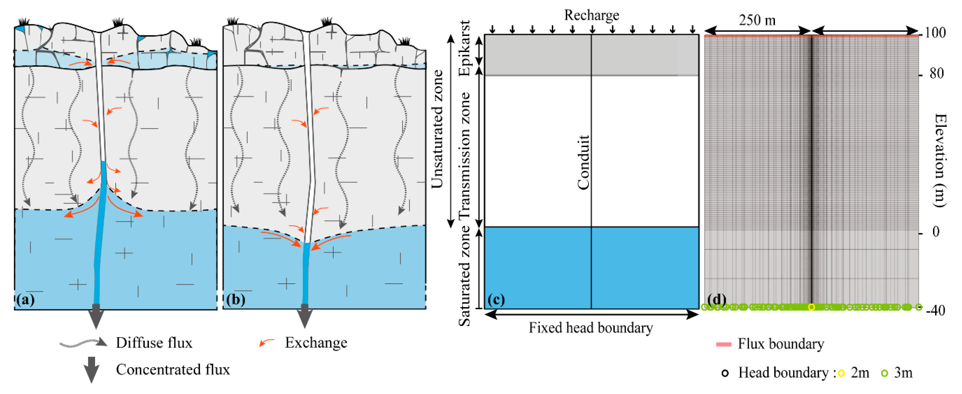
2.1.1. Karst Subsystems

Hydrogeologists commonly subdivide the karst medium into four main vertical subsystems on the basis of geomorphology, hydrodynamic properties, and flow processes [1]: (i) soil and non-karst terrain, (ii) the epikarst [11,37,38], (iii) the transmission zone [39], and (iv) the saturated zone. Thus, the unsaturated zone encompasses soil, the epikarst, and the transmission zone (Figure 1). Though this conceptual model has the advantage of being relatively generic, it remains primarily qualitative [40,41]. Some papers contributed to specify hydrodynamic behaviors for each subsystem [10,42,43]. However, most authors face difficulty in accessing the input and output of each subsystem. Particularly, the functioning of the transmission zone is generally not distinguishable from one epikarst [43] and/or one saturated zone [42].

The epikarst is the near-surface and altered karst zone [37]; its thickness ranges from 0 to approximately 20 m [37,38,44,45]. Alteration processes increase porosity and hydraulic conductivity [11,38]. Hydraulic conductivity may be higher than 10⁻⁵ m/s and effective porosity ranges from 1% to 10% [46,47]. Due to its relatively high porosity and hydraulic conductivity compared to those of the underlying rock, the epikarst can store a large amount of water in locally perched aquifers that generally drain horizontally towards preferential flow paths [11,48,49]. Three factors affect water storage in the epikarst: (1) its thickness and lateral continuity, (2) its average porosity, and (3) the relative rates of inflow and outflow of water [45].

The transmission zone connects and transfers water from the epikarst to the saturated zone with flow essentially vertical through fractures or caves at the subsystem scale. Hydraulic conductivity for the transmission and saturated zones generally ranges between 10⁻⁷ m/s and 10⁻⁴ m/s, and porosity is usually less than 2% [45]. The transmission zone may also play a storage role [50,51], releasing water during the low water period [52].

Assessing the equivalent hydraulic conductivity on a flow unit of such media is not straightforward. Most of the values found in the literature (

Table 1. Value ranges for the properties of karst systems and karst modeling reported in the literature and model parameters.

Subsystem	Property (Units)	Values and Ranges of Values 1 from Literature [References]	Model’s Values and Range of ValuesMin–Ref–Max
Epikarst (EK)	Thickness ThkEK (m)	(0; >30) [45] (few meters; 10−15) [38] (3; 10) [37] (8; 12) [44]	0–20–35
	Porosity ϕEK (-)	(0.05; 0.1) [45,55] (0.1; 0.3) [47] >0.2 [37]	0.01–0.1–0.25
	Horizontal 2 hydraulic conductivity KEK (m/s)	(10−7; 10−4) [13] 10−5 [56] (5 × 10−5; 10−3) [57] (2 × 10−4; 2 × 10−3) [58] 10−3 [59] >1000*KTZ-SZ [60]	10−5–10−2–10−1
Transmission and saturated zones (TZ-SZ)	Thickness ThkTZ (m)	depending on the field site, usually tens of meters, <20; <50 [59] up to 700 [61]	30–80–130
	Porosity ϕTZ-SZ (-)	(0.004; 0.01) [37] 0.005 [62] (0.01; 0.02) [63] (0.024; 0.3) [64]	0.005–0.01–0.025
	Horizontal 2 hydraulic conductivity KTZ-SZ (m/s)	(10−10; 7 × 10−5) [64] (10−7 [18]; 10−6 [19,37]) [57] (5 × 10−7; 5 × 10−6 [56]) [65] (10−6 [19,37]; 10−4 [62]) [63] (10−5; 10−3) [17]	10−7–10−5–10−3
Conduit (C)	Diameter D (m)	(0.08; 15) [29] (2; 10) [33]	Flow Capacity AC * KC (m3/s−1) 10−2–10−1–101
	Section AC (m2)	(<1; >100) [66]
	Hydraulic conductivity KC (m/s)	(6 × 10−5; 4 × 10−1) [64] (10−1; 10) [17,57] (3; 10) [63] 10 [19,65]
Van Genuchten Model	Coefficient α (m−1)	(3.28 × 10−3; 6.23 × 10−1) [15] 3.65 × 10−2 [19,21] 10−2 [17,18]	3.65 × 10−2
	Empirical parameter n (-)	(0.01; 3) [15] 1.83 [19,21] 2 [17,18]	1.83
	Residual water content θr (-) or Residual water saturation Sr (-)	θr = Sr = 0 [18] θr ∈(0.01; 0.05) [15] Sr = 0.05 [19] θr = 0.171 [17]	Sr = 0.05

¹ Ranges of values from the literature are shown in parentheses. ² When anisotropy is considered, values concordant to the strata are presented.

) are not related to a given measurement volume, nor the medium under consideration, which may include all or parts of the fractures and conduits. Moreover, very few studies address anisotropy even qualitatively, and even less vertical anisotropy, which largely controls the occurrence of perched and confined layers [53]. Matrix permeability is recognized to be anisotropic and higher in the dipping direction due to geological layering, with the vertical anisotropy ratio (permeability normal to the strata over permeability concordant with the strata) usually between 0.01 and 1 [54]. Alteration processes, such as fracturing, weathering, or dissolution, likely reduce or possibly reverse this vertical anisotropy of hydraulic conductivity. Due to the confinement of most of the fractures to mechanical units in sedimentary rocks, fractures are systematically wider than they are high and, except larges faults, rarely cut horizons inducing matrix vertical anisotropy [54]. Therefore, fractures increase horizontal anisotropy but affect the vertical anisotropy to a limited extent, notably in thick flow units, such as the transmission zone. It is generally assumed that karst genesis increase mainly the vertical conductivity in the unsaturated zone. However, several processes such as subaerial exposure, dissolution at the water table, or the development of karst inception features can also increase the horizontal permeability in the unsaturated zone. For instance, karst features such as lapies, exemplify the near-surface increase in vertical hydraulic conductivity. They also induce an increase in horizontal permeability and horizontal anisotropy. The net effect of these changes on the resulting vertical anisotropy is uncertain. Hence, it may be considered that: (i) the vertical karst conduits support a large part of the vertical hydraulic conductivity, (ii) these features aside, the epikarst is less anisotropic than the rest of the unsaturated zone [48].

Table 1 provides a literature review of ranges for hydrodynamic parameters in karst subsystems. It serves as a basis for defining parameters of the models of this study. These parameters are also presented in Table 1.

2.1.2. Matrix vs. Conduit Properties

Whatever the subsystem, the karst medium is a complex heterogeneous and discontinuous spatial distribution of more or less connected entities; these entities range across a continuum from the less fractured porous matrix with high capacity and low hydraulic conductivity to karst conduits with low capacity and high hydraulic conductivity. Microporous matrix hydraulic conductivity usually ranges from 10⁻¹² to 10⁻⁶ m/s (assuming that permeability of 1 Darcy is equivalent to a hydraulic conductivity of 10⁻⁵ m/s) at a small scale [67,68], while the conduits hydraulic conductivity is greater than 10⁻¹ m/s [69].

Modelers usually distinguish slow or diffuse and fast or concentrated flows in all karst subsystems. The overall fast to slow flow ratio depends on karst maturity. The portion of concentrated recharge into conduits ranges from 5% for young karst to 40–58% for mature karst [13,63,65,70,71]. However, this ratio is difficult to quantify because exchanges between capacitive and conductive parts of the karst system vary as a function of space and time. Chang et al. [71] highlight the important role of the epikarst in the recharge repartition and show its impact on hybrid models simulations.

It is generally considered that the conduits supply the continuum during high flow periods (Figure 1a) whereas they drain the surrounding continuum during low flow periods (Figure 1b) [10,11,48,72]. Such exchanges depend directly on local pressure gradients. Characteristics of conduits (e.g., diameter, hydraulic conductivity) affect also hydraulic head distribution [73,74,75,76]. However, increasing the flow capacity of the conduits above a certain threshold in saturated conditions does not affect the response of the model [74].

Figure 1. Schematic representation of water flux and exchanges through karst as a function of the hydrological period and corresponding numerical model. (a) High flow conceptual model: the conduits drain the upper continuum and supply the lower continuum; (b) Low flow conceptual model: the conduits drain the surrounding continuum; (c) subsystems of the numerical model; (d) associated mesh with boundary conditions.

Figure 1. Schematic representation of water flux and exchanges through karst as a function of the hydrological period and corresponding numerical model. (a) High flow conceptual model: the conduits drain the upper continuum and supply the lower continuum; (b) Low flow conceptual model: the conduits drain the surrounding continuum; (c) subsystems of the numerical model; (d) associated mesh with boundary conditions.

2.2. Modeling Approach

The following sections present the 3D hybrid model constructed to study the interactions between matrix and conduits during a recharge event. This finite element model was developed with FEFLOW 7.0 by DHI WASY (https://www.mikepoweredbydhi.com/products/feflow) [35,77].

2.2.1. Model Description, Boundary Conditions, and Evaluation Criteria

The model represents the matrix surrounding a vertical conduit along the unsaturated zone and a part of the saturated zone (Figure 1c,d). The vertical conduit is located in the center of a 1 km² square so that the lateral boundaries are far enough from the conduit to have little effect on near-conduit exchanges. Hence, the presented results focus on a smaller area, up to 250 m from the conduit (e.g., Figure 2). The model is 140 m thick (from z = −40 m to z = 100 m) including the epikarst, transmission zone, and the upper part of the saturated zone. The model grid has 1405 vertex per slice and 104 slices. From the top of the model to a depth of 100 m, the layers are 1 m thick. The three deeper layers that correspond to the permanently saturated interval are thicker. They constitute a buffer zone to avoid a significant impact of the boundary conditions. The horizontal mesh is refined all around the vertical conduit.

In terms of boundary conditions, a recharge flux is applied on the top of the model (z = 100 m) whereas Dirichlet boundary conditions control the discharge at the base of the model (z = −40 m). The recharge is uniform, i.e., without a focused recharge point on discrete features, but varies as a function of time. The same single recharge event is simulated for the various parameter sets. It consists of 100 mm in two days (the third and fourth days) represented by an isosceles triangle reaching 100 mm/day in one day (Figure 3a). This single recharge event adds to a constant recharge of 0.5 mm/day which steady-state response constitutes the initial condition of the transient simulation. This single event is realistic as observed in the Mediterranean climate for instance [78,79]. At the base of the model, constant hydraulic heads of 3 m and 2 m are applied to vertex corresponding to matrix and conduits, respectively (Figure 1d). This difference between matrix and conduit ensures preferential flow towards the conduit at the base of the model for mean steady recharge. No-flow boundary conditions are applied to the vertical faces of the model.

The simulations results are assessed by qualitative comparison to conceptual models from the literature and quantitative inter-comparison.

2.2.2. Flow Equations and Model Parameters

Hybrid models make it possible to consider independent flow physics for the continuum (e.g., Darcy’s law or Richards’ equation) and discrete features (e.g., Hagen-Poiseuille, Darcy-Weisbach, Manning-Strickler equations, or Darcy’s law). The most complex but also most realistic case would couple the Richards’ equation within the continuum to the Manning-Strickler equation in the discrete features [35,70,80]. Several tests revealed that this configuration hinders convergence of the model. In this study, although failure to account for turbulent flows in discrete features may affect the overall response [29,30], Richards’ equation and Darcy’s law are considered for continuum and discrete features, respectively, as an acceptable compromise between numeric efficiency and realism. Flows in the matrix are assumed to obey the Richards’ equation [81], which makes it possible to reproduce the variably saturated water flow:

$$\frac{\partial }{\partial \mathrm{x}}\left[\mathrm{K}{\left(\mathsf{\psi }\right)}_{\mathrm{xx}}\frac{\partial \mathrm{h}}{\partial \mathrm{x}}\right]+\frac{\partial }{\partial \mathrm{y}}\left[\mathrm{K}{\left(\mathsf{\psi }\right)}_{\mathrm{yy}}\frac{\partial \mathrm{h}}{\partial \mathrm{y}}\right]+\frac{\partial }{\partial \mathrm{z}}\left[\mathrm{K}{\left(\mathsf{\psi }\right)}_{\mathrm{zz}}\frac{\partial \mathrm{h}}{\partial \mathrm{z}}\right]\pm \mathrm{U}=\frac{\partial \mathsf{\theta }}{\partial \mathrm{t}}$$

(1)

for the case when anisotropy and coordinate axes are parallel, where θ is the volumetric water content (-), t is time (s), x, y, and z are the spatial coordinates (m) (positive upwards), K(Ψ) is the unsaturated hydraulic conductivity (m/s) in the function of the pressure head Ψ (m), h is the hydraulic head (m), with h = Ψ + z, and U is the sink-source term (s⁻¹). Solving the Richards’ equation requires constitutive relationships for saturation as well as the relative hydraulic conductivity. Several models based on statistical pore-size distribution have been developed [82,83,84,85,86,87]. Their application and calibration mostly concern unconsolidated porous media [88]. The literature contains a few applications of the Van Genuchten model [85] to a carbonate matrix [15,18,19,21]. However, the application of this empirical model to a fractured or karstified carbonate matrix is not well documented. In fact, estimating the relationship between saturation and relative hydraulic conductivity for karst media remains a challenge [89]. Here the Van Genuchten model is therefore applied with constant and uniform parameters from the literature for all simulations (Table 1). For the unsaturated zone, water content is equal to:

$$\mathsf{\theta }\left(\mathsf{\psi }\right)={\mathsf{\theta }}_{\mathrm{r}}+\frac{{\mathsf{\theta }}_{\mathrm{s}}-{\mathsf{\theta }}_{\mathrm{r}}}{{\left[1+{\left(\mathsf{\alpha }\mathsf{\psi }\right)}^{\mathrm{n}}\right]}^{\mathrm{m}}}$$

(2)

where θ_r and θ_s are residual and saturated water contents (−), respectively, and α (cm⁻¹), n, and m are empirical parameters. Note that setting either residual water content θ_r or residual saturation S_r is equivalent because the two parameters are linked: moisture content θ equals porosity ϕ multiplied by saturation S. However, some confusion may exist in the literature with residual saturation values directly set as equal to residual water content values [19] (Table 1). The relative hydraulic conductivity K_r (-) in the unsaturated zone follows this relation:

$${\mathrm{K}}_{\mathrm{r}}={\mathrm{S}}_{\mathrm{e}}^{0.5}{\left[1-{\left(1-{\mathrm{S}}_{\mathrm{e}}^{\frac{1}{\mathrm{m}}}\right)}^{\mathrm{m}}\right]}^2$$

(3)

S_e is effective saturation, generally defined as [85]:

$${\mathrm{S}}_{\mathrm{e}}=\frac{\mathsf{\theta }-{\mathsf{\theta }}_{\mathrm{r}}}{{\mathsf{\theta }}_{\mathrm{s}}-\mathsf{\theta }\mathrm{r}}=\frac{\mathrm{S}-{\mathrm{S}}_{\mathrm{r}}}{1-\mathrm{Sr}}$$

(4)

In the model, conduits are always fully conductive and follow Darcy’s law. Thus, flux through the conduit is proportional to both cross-section and hydraulic conductivity of the conduit. Variations of these two parameters are therefore redundant. We thus consider the flow capacity, defined by the product of the cross-section area by hydraulic conductivity, as the key parameter for flow in conduits. The discrete features can be regarded as preferential pathways embedded in the equivalent porous medium. Discrete features and porous medium are supported by the same vertex where hydraulic heads are computed. Flow equations are solved simultaneously for both discrete features and regular mesh as if edges supporting discrete features were additional mesh cells. Exchanges between these two objects are therefore implicit [35].

We selected the values of model properties (Table 1) based on the literature. We focused on the effect of the following varying parameters: thickness (Thk), porosity (Φ), and horizontal hydraulic conductivity (K) of the epikarst (EK) and transmission zone (TZ) respectively, and flow capacity of the conduit. Values for the epikarst (Φ_EK, K_EK) are distinguished from those for the transmission and saturated zone that are equal (Φ_TZ−SZ, K_TZ−SZ). Assuming that the discrete feature supports most of the vertical conductivity induced by the karst and considering the contrast of anisotropy between the epikarst and transmission zone, hydraulic conductivity is set isotropic in the epikarst whereas it is set anisotropic everywhere else, with a horizontal conductivity ten times greater than the vertical, as frequently considered [54]. Note that the thickness of the epikarst (Thk_EK) does not vary during the simulation whereas the thicknesses of the transmission zone and saturated zone may vary because of flooding of the epiphreatic zone. We thus consider the initial thickness of the transmission zone as the parameter of interest (Thk_TZ). These parameters are modified around a reference simulation. The parameter values are in the range defined in Table 1. Only one parameter is changed at a time.

Setting the flow capacity of the conduit is a tricky process. Indeed, in hybrid models, discrete elements are of interest especially for representing major conduits with high flow capacity. However, two conductive discrete features cause a matrix-restrained flow regime and act as fixed-head boundary conditions that would be more computationally efficient [74]. Thus, discrete features are of interest only if their flow capacity ensures both a high contrast with matrix characteristics and a conduit-influenced flow regime as defined by Kovács et al. [74]. Here, considering the scale of the model and some preliminary simulations, we tested values between 10⁻² and 10¹ m³/s⁻¹ (Table 1 and Figure 4).

3. Results

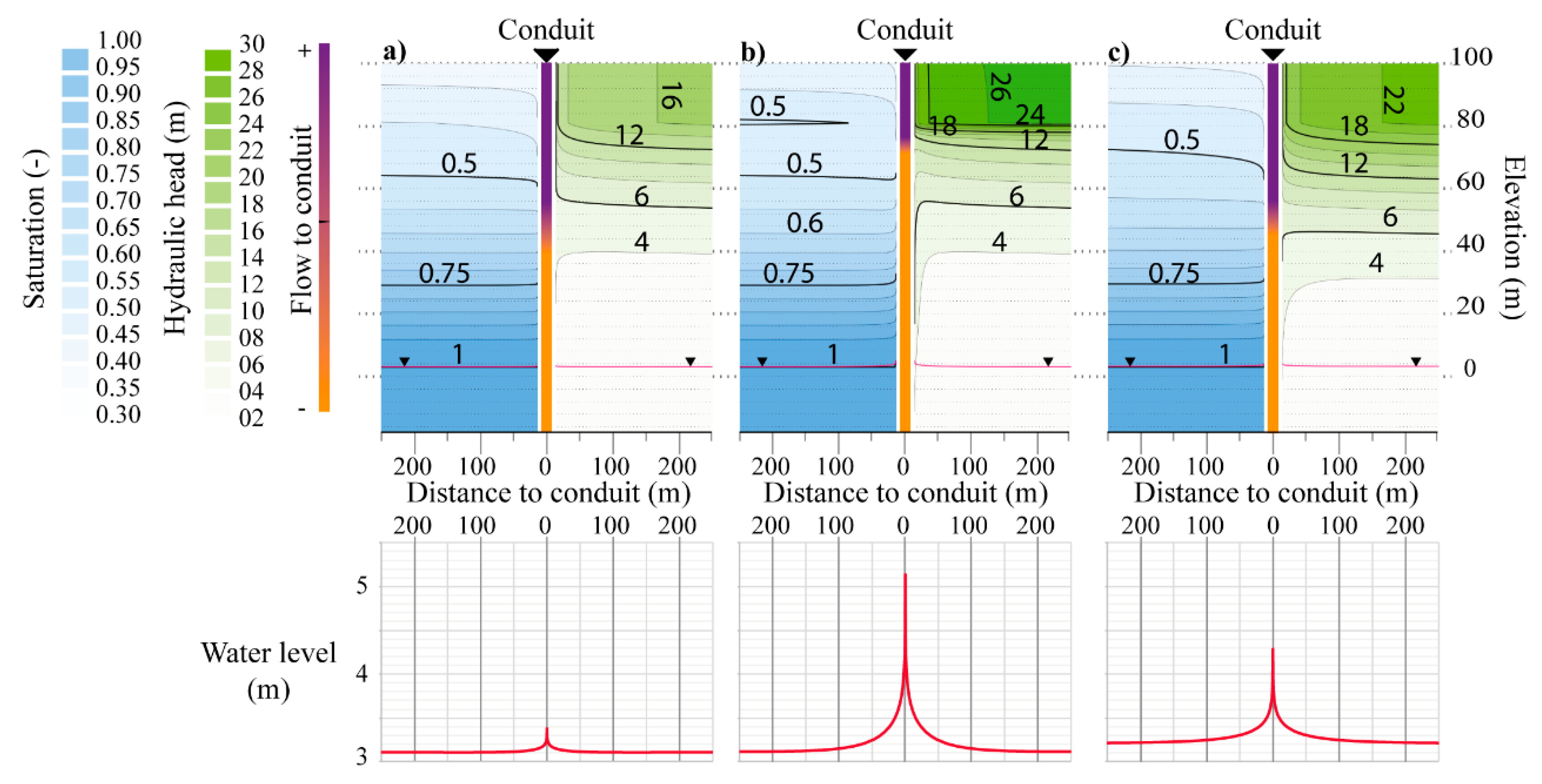
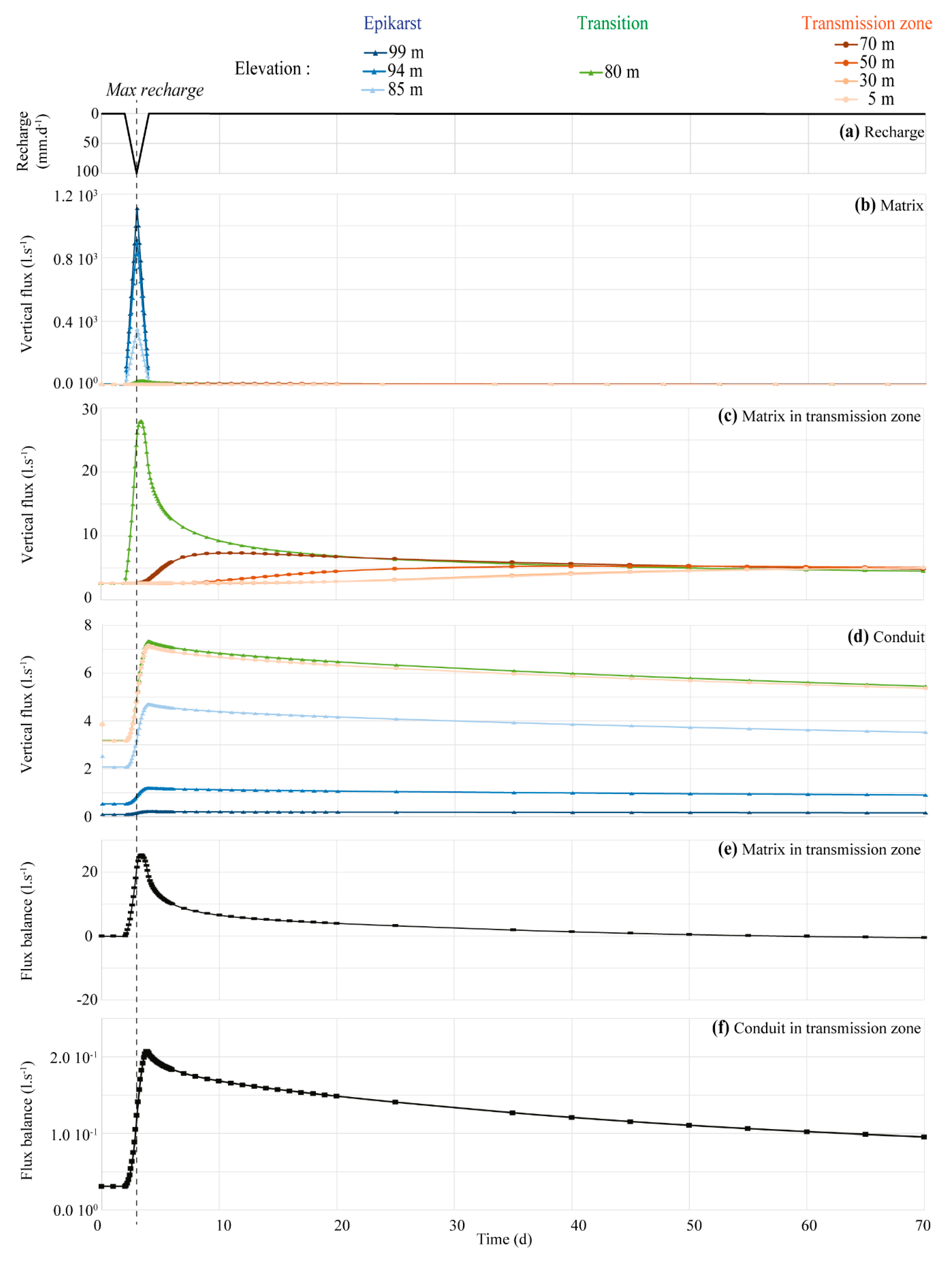
3.1. Spatio-Temporal Evolution of the Flows at the Conduit Scale

We investigated the spatial and temporal variation of the governing flow processes during the recharge event based on cross-sections of the saturation and hydraulic head. Figure 2 shows these profiles for the reference simulation at different times: at initial steady-state, at the end of the recharge event, and 77 days after the recharge event. Whatever the time, in the epikarst, water flows horizontally towards the conduit whereas the flow through the transmission zone (TZ) is mainly vertically oriented, as highlighted in the literature [1,3,48] and summarized in Figure 1a,b. The velocity field could therefore seem counter-intuitive given the anisotropy of each subsystem. However, it is mainly driven by both larger scale heterogeneity due to the contrast between subsystems and pressure at the base of the transmission zone and along the conduit.

Figure 2. Profiles of the saturation (blue) and hydraulic head (green) around the conduit, with plots zooming on the water level at three time steps: (a) at steady state before the recharge event, (b) at the end of the recharge event, (c) 77 days after the event.

Figure 2. Profiles of the saturation (blue) and hydraulic head (green) around the conduit, with plots zooming on the water level at three time steps: (a) at steady state before the recharge event, (b) at the end of the recharge event, (c) 77 days after the event.

The flow through the transmission zone is diffuse and causes the water level on the top of the saturated zone to increase up to almost 10 cm far from the conduit (Figure 3d). The water level near the conduit increases also due to concentrated flow in the conduit, which slightly accentuates the piezometric dome near the conduit (Figure 3c).

Exchanges between the matrix and conduit also vary with depth and time. As expected, the conduit always drains the matrix at the top of the model. Despite a lower fixed head at the conduit boundary that could induce drainage through the whole conduit, the conduit partially supplies the matrix in the transmission zone. The depth of inversion of flux between the matrix and conduit remains relatively shallow. Even in steady-state, the conduit does not drain the matrix in the epiphreatic zone. The constant recharge probably prevents reaching the low flow as shown in Figure 1b. However, at the end of the recharge event, although the conduit is highly conductive and the boundary conditions at the bottom of the model differ between conduit and matrix, the matrix drains the conduit throughout almost the entire transmission zone. This result contrasts with the common representation of conduits draining water toward the saturated zone, probably largely influenced by results in saturated conditions [74]. The zone influenced by this flow from the conduit towards the matrix is nevertheless limited to the close vicinity of the conduit.

Figure 3 confirms observations from the profiles. In the epikarst, the vertical flux through the horizontal section of the matrix decreases rapidly as a function of depth (Figure 3b) in favor of the flow transited by the conduit (Figure 3d). Consequently, the flux transited by the matrix is about forty times lower in the top of the transmission zone (Figure 3c) than in the epikarst. The transmission zone delays and flattens the matrix flux, which causes temporary storage in the medium. This is highlighted in Figure 3e which presents the flux balance of the matrix in the transmission zone, i.e., the difference between the flux into and out of the matrix in the transmission zone, as a function of time. Exchanges between the matrix and conduits are limited or almost balanced in the transmission zone. Indeed, whatever the time, the flux transited by the conduit at the bottom (5 m elevation) of the transmission zone is slightly smaller than the one at the top (80 m elevation) of this zone (Figure 3c) and the flux balance in the conduit (the difference between the flux into and out of the conduit in the transmission zone) is always smaller than 0.21 L/s⁻¹ (Figure 3f). Here, water from the conduit wet the unsaturated medium surrounding the conduit. However, the total flux from the conduit to the transmission zone remains below 3% of the flux entering the transmission zone by the conduit. As observed on the profiles, the influence on flows in the transmission zone remains limited to the area close to the conduit.

Figure 3. Vertical flux through horizontal planes at different elevations and mass balances, in the matrix and conduit respectively, as functions of time. (a) Recharge at the top of the model (b) Flux through a horizontal matrix section at different elevations in both the epikarst and transmission zone. (c) Flux through a horizontal matrix section at different elevations in the transmission zone only with an adapted scale. (d) Flux through a horizontal conduit section at different elevations in both the epikarst and transmission zone. (e) Flux balance of matrix in the transmission zone. (f) Flux balance of a conduit in the transmission zone.

Figure 3. Vertical flux through horizontal planes at different elevations and mass balances, in the matrix and conduit respectively, as functions of time. (a) Recharge at the top of the model (b) Flux through a horizontal matrix section at different elevations in both the epikarst and transmission zone. (c) Flux through a horizontal matrix section at different elevations in the transmission zone only with an adapted scale. (d) Flux through a horizontal conduit section at different elevations in both the epikarst and transmission zone. (e) Flux balance of matrix in the transmission zone. (f) Flux balance of a conduit in the transmission zone.

At the base of the epikarst, far from the conduit, saturation increases rapidly during the recharge event and decreases slowly after it (Figure 2). The vertical conduit finally drains the water temporarily stored there. This configuration does not produce a locally perched aquifer, as referred to in the literature. Nevertheless, these results highlight several factors that may favor the occurrence of locally saturated zones in the epikarst: the distance from the conduit and contrasts of hydraulic conductivity. More important (repeated, longer, or more intense) recharge events and topographic variations of the interface between the epikarst and the transmission zone likely favor these phenomena too. The impact of varying parameters on saturation at the bottom of the epikarst is discussed hereafter.

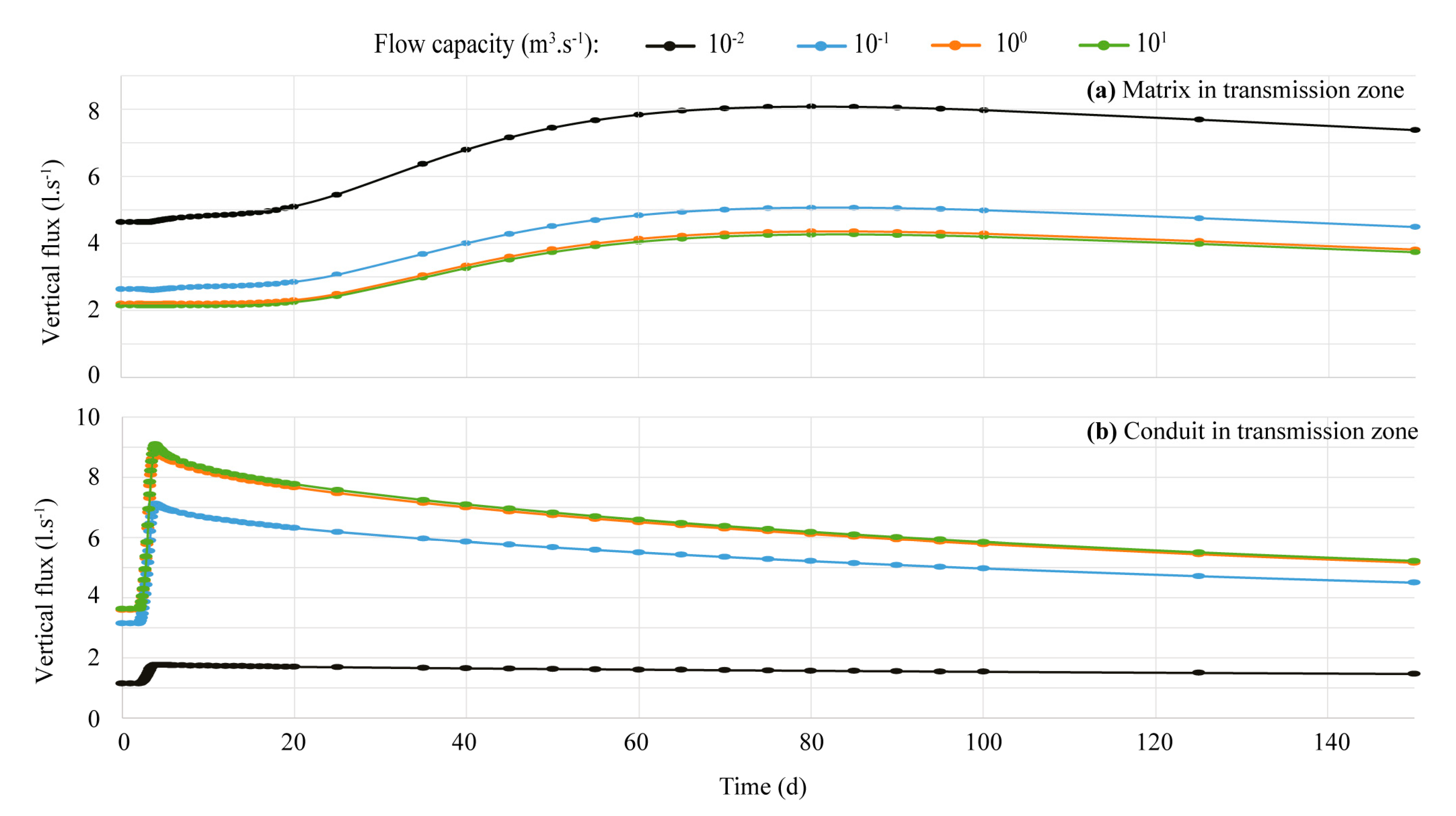
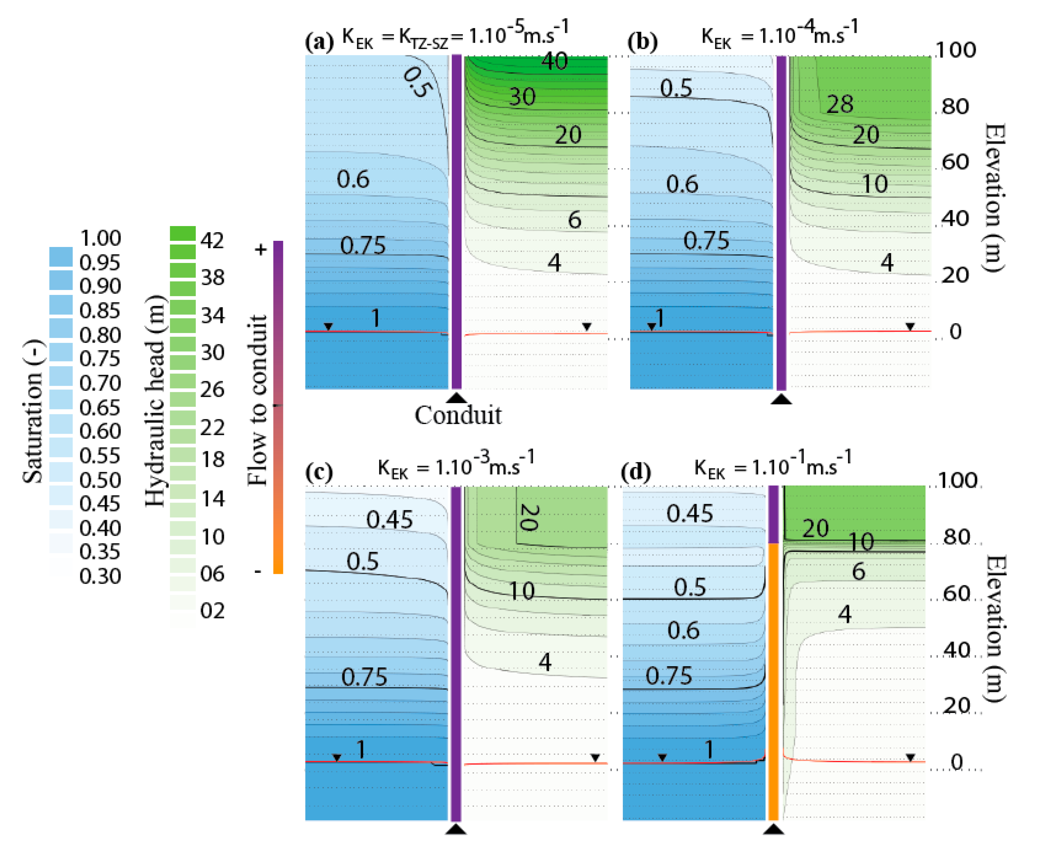
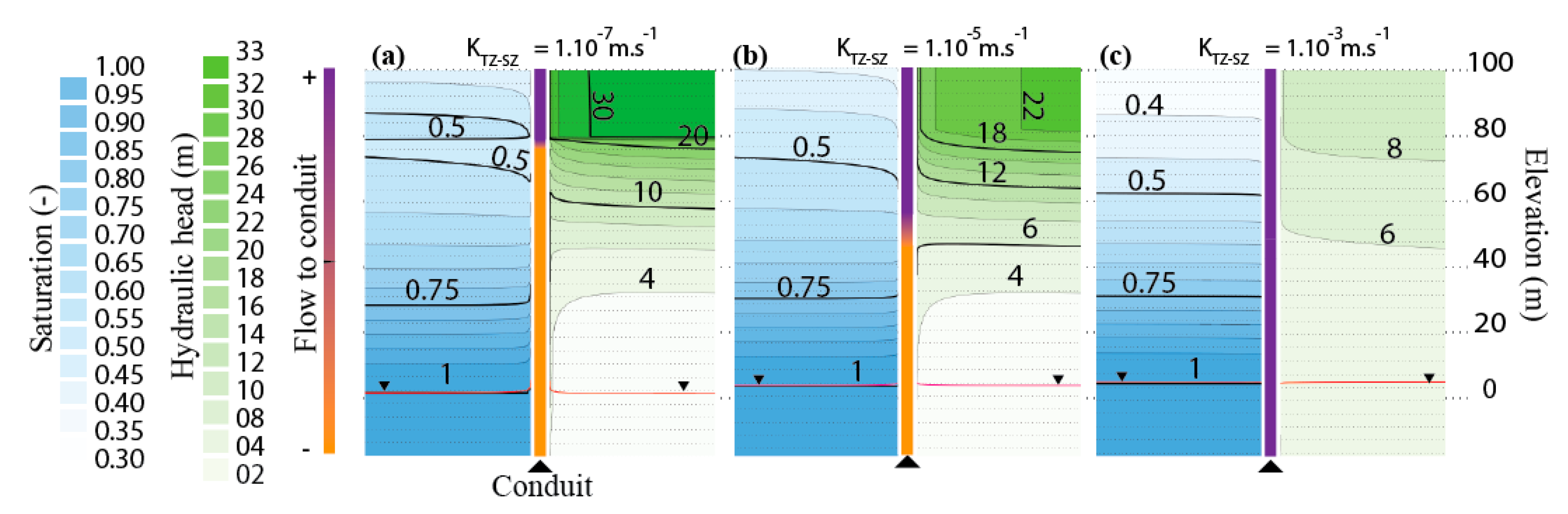
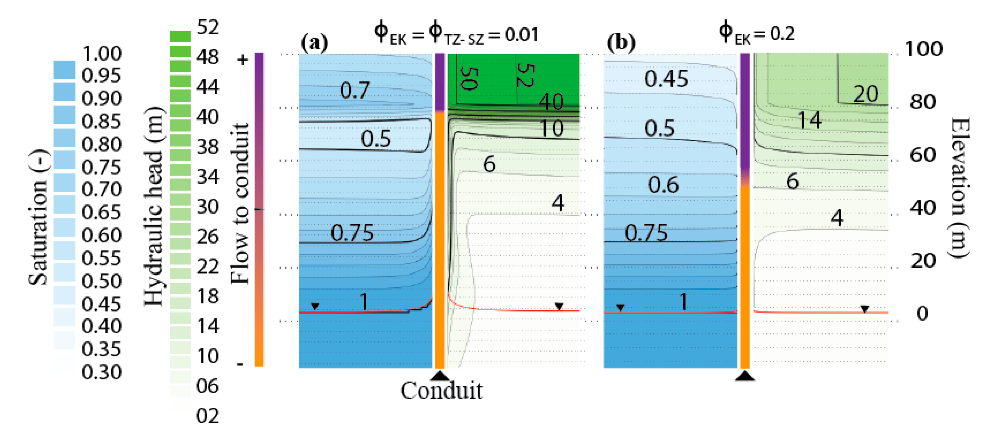
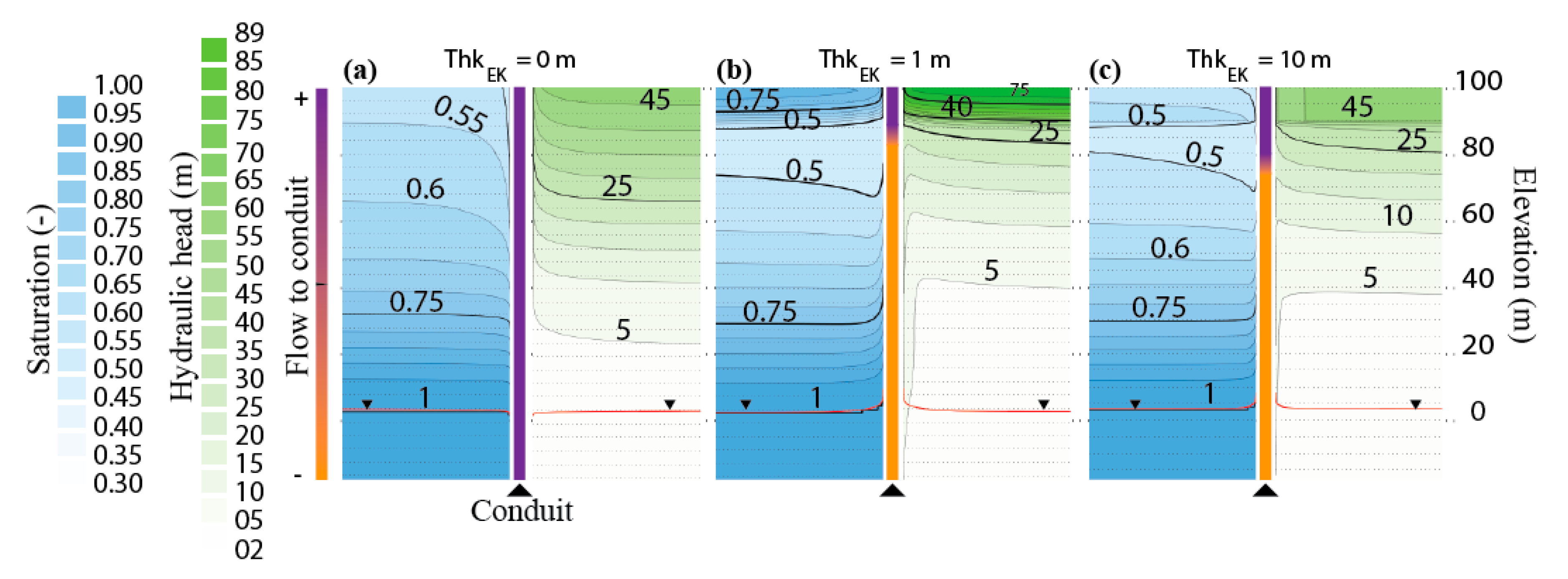
3.2. Impact of Parameter Variation at the Conduit Scale

The effect of the extreme values of the flow capacity of the conduit is limited. Obviously, a too-small value of flow capacity (here, 10⁻² m³/s⁻¹) limits the preferential flow through the conduit (Figure 4). Conversely, increasing the flow capacity of the conduits above a threshold value (here, 1 m³/s⁻¹) does not have a greater impact on the response of the model, as referred to by Kovács et al. [74] for saturated conditions. We have therefore selected an intermediate value (10⁻¹ m3/s⁻¹) for the reference model, to simulate a highly conductive conduit that ensures preferential flow but whose effect differs from that of a fixed-head boundary condition.

Figure 4. Vertical flux through the horizontal plane at the base of the transmission zone as a function of time, in the matrix (a) and conduit (b) respectively, for four values of flow capacity in the conduit.

Figure 4. Vertical flux through the horizontal plane at the base of the transmission zone as a function of time, in the matrix (a) and conduit (b) respectively, for four values of flow capacity in the conduit.

Figure 5, Figure 6, Figure 7 and Figure 8 show profiles of the saturation and hydraulic head for different varying parameters. Each profile is taken at the time step for which the flux at the bottom output of the model is maximum. Figure 5 shows four profiles of the saturation and hydraulic head for different values of K_EK (from 10⁻⁵ to 10⁻¹ m/s) while K_TZ−SZ (10⁻⁵ m/s) and other parameters remain constant. Conversely, Figure 6 shows three profiles of the saturation and hydraulic head for different values of K_TZ−SZ (from 10⁻⁷ to 10⁻³ m/s) while K_EK and other parameters remain constant (10⁻² m/s). The contrast of hydraulic conductivity between the epikarst and transmission zone mainly controls the flow direction in the epikarst during the recharge event. Other things being equal, a ratio of hydraulic conductivity higher than ten (one hundred for the ratio of vertical conductivity due to the difference of anisotropy) ensures horizontal preferential flow through the epikarst toward the conduit while saturation monotonically increases as a function of depth (Figure 5a versus Figure 8b,c). A ratio greater than about 10⁴ is necessary to distinguish clearly specific behaviors in the epikarst as compared to the transmission zone: local saturation is higher at the bottom of the epikarst, sharp variation of flow direction between both zones, and the conduit is supplying the matrix in the transmission zone (Figure 5d and Figure 6a).

Varying porosity in the epikarst (Figure 7) also affects the flow and saturation repartition in the entire medium. Although it is difficult to compare the logarithmic variation of hydraulic conductivity with the linear variation of porosity, the impact of the latter is greater in the range of realistic values for both parameters. It is presumably due to the combined effects of porosity on both saturation and effective conductivity, in accordance with the application of the Richards’ equation and the Van Genuchten empirical model. Indeed, for the same amount of incoming water, the lower the porosity values, the higher the saturation and the effective conductivity. Lower porosity values thus yield lower local effective storage and transit time.

Figure 7. Profiles of the saturation (blue) and hydraulic head (green) around the conduit for various values of porosity of the epikarst. Each profile is taken at the time step for which the flux at the bottom output of the model is maximum. (a) The porosity is the same throughout the entire model and equal to 0.01. (b) The epikarst porosity is equal to 0.2.

Figure 7. Profiles of the saturation (blue) and hydraulic head (green) around the conduit for various values of porosity of the epikarst. Each profile is taken at the time step for which the flux at the bottom output of the model is maximum. (a) The porosity is the same throughout the entire model and equal to 0.01. (b) The epikarst porosity is equal to 0.2.

Various values of thickness were also tested for the epikarst and the transmission zone. Figure 8 shows profiles of the saturation and hydraulic head for three different values of thickness of the epikarst. The thickness of the entire system remains constant and the thickness of the transmission zone varies consequently. Note the specific case of a null thickness corresponding to the absence of the epikarst (Figure 8a). The three results are very different. For a sufficient thickness, here above 10 m, the profiles have all the features mentioned above, notably horizontal flow towards the conduit in the epikarst, the supply of the matrix through the conduit at depth, and a higher saturation far from the conduit at the base of the epikarst. A decreasing thickness of the epikarst causes decreasing storage capacity and, for the same recharge event, the saturation and hydraulic head reach higher values with higher gradients. The flow features (horizontal flow towards the conduit in the epikarst, the supply of the matrix through the conduit at depth) are preserved even for a thin epikarst (Figure 8b) because the interface between the epikarst and the transmission zone acts as a hydraulic barrier. Indeed, the saturation contrast created by the recharge event enhances the conductivity contrast between the two subsystems. Thus, the top of the transmission zone remains poorly saturated, therefore not very conductive, while preferential flows drain water towards the conduit in the more conductive epikarst. However, the shape of the saturation profiles varies with the epikarst thickness. The formation of a zone with higher saturation far from the conduit at the base of the epikarst requires a sufficient epikarst thickness. Without the epikarst (Figure 8a), the resulting profiles are very different, with higher saturation values at the top of the transmission zone, a monotonous variation of saturation, and the repartition of flows towards the conduits all along the transmission zone. Thus, notably due to unsaturated conditions and whatever its thickness, the epikarst appears to be a key feature for concentrating water towards conduits in addition to geomorphology and topography which also promote such processes in real karst systems.

Figure 8. Profiles of saturation (blue) and hydraulic head (green) around the conduit for various thicknesses of the epikarst. Each profile is taken at the time step for which the flux at the bottom output of the model is maximum. (a) Model without an epikarst. (b) Model with a 1 m thick epikarst. (c) Model with a 10 m thick epikarst.

Figure 8. Profiles of saturation (blue) and hydraulic head (green) around the conduit for various thicknesses of the epikarst. Each profile is taken at the time step for which the flux at the bottom output of the model is maximum. (a) Model without an epikarst. (b) Model with a 1 m thick epikarst. (c) Model with a 10 m thick epikarst.

Varying the thickness of the transmission zone provides similar profiles of the hydraulic head (not presented here), with lower heads for lesser thicknesses. Higher thickness of the transmission zone causes lower saturation and consequently lower effective conductivity at the top of this zone, in accordance with Richards’ equation. Therefore, the hydraulic conductivity contrast at the interface between the epikarst and transmission zone is higher, which favors the development of a local maximum saturation at the base of the epikarst. The drainage radius of the conduit and flow anisotropy also increases as the thickness of the transmission zone increases.

Finally, the transmission zone largely affects the distribution of pathways and transit times between the matrix and conduits. On the one hand, by contrast with the epikarst properties, it could act or not as a barrier that reinforces horizontal drainage towards conduits in the epikarst. On the other hand, the transmission zone directly competes with the vertical conduit to flow water from the epikarst to the saturated zone.

4. Discussion

We performed numerical experiments to evaluate the ability and interest of hybrid models to represent flow processes in subsystems of the karst unsaturated zone and the associated matrix-conduits exchanges. We built the model with the aim of reproducing commonly accepted conceptual models while setting parameter values consistent with the literature. The assessment of model results is based on qualitative comparisons of cross-sections of simulated saturation and hydraulic head with conceptual representations from the literature illustrated in Figure 1. Our results show that hybrid models are capable of reproducing most accepted features of karst hydrodynamics in an unsaturated zone: storage and distribution of recharge in the epikarst, flow concentration towards conduits in the epikarst, intensity and direction of exchanges between the matrix and conduit that vary in time and space. The consideration of an epikarst layer and the contrast of effective conductivity between the epikarst and transmission zone are key elements for enhanced flow simulation in the karst unsaturated zone. Moreover, this model gives some insights to understand and quantify the effect on flow processes of parameter variation in each subsystem. This opens the door to testing reservoir-scale applications including complex networks of karst conduits [90].

Using Richards’ equation and the Van Genuchten model to consider variably saturated flow also appears to be very useful in reproducing these processes, including saturation that varies in time and space. Several tests not presented here confirm that saturation front displacement and perched aquifers are likely impossible to simulate with simplified representations of unsaturated flows that use pseudo-saturation [91], such as those available in FEFLOW [35]. Applying the Richards’ equation to the continuum has nevertheless led us to simplify the representation of flows in the conduits without simulating turbulent flows. If the consideration of turbulent flow is needed for correctly modeling large-scale saturated aquifers with small or rough conduits [30], the configuration and the subsequent needs are completely different here: a variably saturated medium with a major conduit is considered at mesoscale. The consistency between the simulations results and both observations and concepts issued from real karst systems, as well as the wide spectrum of responses obtained, lead us to consider that the major features have probably been identified and that hybrid models allow realistic simulations of unsaturated flow processes near karst conduits. However, addressing the issue of considering turbulent flow in the conduit together with the variably saturated flow in the continuum and, in general, enhancing and upscaling physically-based modeling of flows in both the matrix and conduits of the unsaturated zone, still poses numerical challenges.

On the other hand, parameters of the Van Genuchten model have not been varied due to a lack of information in the literature. The setting of the constitutive relationships for saturation as well as the relative hydraulic conductivity, as the Van Genuchten model, applied to fractured and karstified carbonates is a broad issue whatever the scale of interest. Further progress in this area would require a dedicated study. More generally, setting the parameters of hybrid models appears to be a tricky task. Beyond the usual problems of investigation techniques, data acquisition, and up-scaling largely addressed in the literature [2,25], improving the physics represented in the models has a corollary to define and assess their parameters correctly. The continuum and the discrete elements of hybrid models each support part of the characteristics of the karst medium that must, therefore, be distributed [27]. Some questions remain and are probably case-dependent: what exactly do we represent with discrete elements, geometric objects, or physical processes and how to up-scale them? In the case of the hydraulic conductivity field, for example, it is not only difficult to attribute to each entity a conductivity value that honors the various constraints including suitability for the represented object or process but also to evaluate related parameters such as anisotropy. Additionally, in this hypothetic case, the problem of intra-subsystem heterogeneity has not been addressed. Thus, the availability of models capable of finely representing the physical processes at various scales transforms the paradigm of succeeding in modeling field observations in the question of characterizing the properties of the medium studied for modeling purposes.

5. Conclusions

In this paper, we examined some usual concepts of karst hydrodynamics using a hybrid model. We focused this work on interactions between a fully conductive conduit and the surrounding unsaturated matrix, which have rarely been addressed. We explored a range of parameters from the literature to evaluate the ability of such models to simulate observed processes, to quantify how varying parameters affect these processes, and to identify the key features and parameters of the model. Especially, we focused on the distinction between the epikarst and the transmission zone.

The hybrid model was able to reproduce conceptual representations of karst hydrodynamics at the conduit scale with ranges of parameters commonly accepted in the literature: transient storage and distribution of recharge, flow concentration towards conduits in the epikarst, and matrix-conduit exchanges, with intensity and direction that vary in time and space. Considering variably saturated flow appears to be useful for reproducing most of the processes referenced in the literature. Indeed, saturation varying as a function of time in the matrix also caused a realistic variability in the competition between the matrix and explicit conduits. The study also raised the need to deepen knowledge on the saturation-conductivity relationships in karst media and to develop hybrid models effectively coupling the modeling of unsaturated flows in the matrix to the modeling of turbulent flows in the discrete elements. The recent work opens interesting avenues [23]. Finally, the remaining question is more about the estimation of the scaled properties we need to know to simulate physical processes correctly than how to simulate them.

The various numerical simulations confirmed that the usual distinction between the epikarst and the transmission zone is important for controlling the near-surface flow distribution. The exchanges between the epikarst and the conduit, presented in Section 2.1 and summarized in Figure 1a,b, were properly reproduced and highlighted the important role of the epikarst in distributing the recharge. Our study confirmed that the presence of the epikarst affects not only the distribution of recharge in this zone but also the conduit-matrix interactions in the entire unsaturated zone, as observed by Trček [92]. Moreover, the variation of the effective conductivity related to the variation of saturation in the medium reinforced the contrast between the epikarst and the transmission zone during a recharge event and affected the exchange between the matrix and the conduit in close proximity to the conduit.

References

1. Bakalowicz, M. Karst groundwater: A challenge for new resources. Hydrogeol. J. 2005, 13, 148–160. [Google Scholar] [CrossRef]
2. Hartmann, A.J.; Goldscheider, N.; Wagener, T.; Lange, J.H.M.; Weiler, M. Karst water resources in a changing world: Review of hydrological modeling approaches. Rev. Geophys. 2014, 52, 218–242. [Google Scholar] [CrossRef]
3. White, W.B. Conceptual models for carbonate aquifers. Ground Water 2012, 50, 180–186. [Google Scholar] [CrossRef]
4. White, W.B. Conceptual models for karstic aquifers. In Karst Modeling: Special Publication 5; Palmer, A.N., Palmer, M.V., Sasowsky, I.D., Eds.; The Karst Waters Institute: Charles Town, WV, USA, 1999; pp. 11–16. [Google Scholar]
5. Shuster, E.T.; White, W.B. Seasonal fluctuations in the chemistry of lime-stone springs: A possible means for characterizing carbonate aquifers. J. Hydrol. 1971, 14, 93–128. [Google Scholar] [CrossRef]
6. Shuster, E.T.; White, W.B. Source areas and climatic effects in carbonate groundwaters determined by saturation indices and carbon dioxide pressures. Water Resour. Res. 1972, 8, 1067–1073. [Google Scholar] [CrossRef]
7. Worthington, S.R.H. Groundwater residence times in unconfined carbonate aquifers. J. Cave Karst Stud. 2007, 69, 94–102. [Google Scholar]
8. Smart, P.L.; Hobbs, S.L. Characterisation of carbonate aquifers: A conceptual base. In Proceedings of the Environmental Problems in Karst Terranes and Their Solutions Conference, Dublin, OH, USA, 28–30 October 1986; pp. 1–14. [Google Scholar]
9. Morales, T.; Uriarte, J.A.; Olazar, M.; Antigüedad, I.; Angulo, B. Solute transport modelling in karst conduits with slow zones during different hydrologic conditions. J. Hydrol. 2010, 390, 182–189. [Google Scholar] [CrossRef]
10. Bailly-Comte, V.; Martin, J.B.; Jourde, H.; Screaton, E.J.; Pistre, S.; Langston, A. Water exchange and pressure transfer between conduits and matrix and their influence on hydrodynamics of two karst aquifers with sinking streams. J. Hydrol. 2010, 386, 55–66. [Google Scholar] [CrossRef]
11. Mangin, A. Contribution à l’Étude Hydrodynamique des Aquifères Karstiques. Ph.D. Thesis, Université de Dijon, Dijon, France, 1975. [Google Scholar]
12. Mudarra, M.; Andreo, B. Relative importance of the saturated and the unsaturated zones in the hydrogeological functioning of karst aquifers: The case of Alta Cadena (Southern Spain). J. Hydrol. 2011, 397, 263–280. [Google Scholar] [CrossRef]
13. Perrin, J.; Jeannin, P.-Y.; Zwahlen, F. Epikarst storage in a karst aquifer: A conceptual model based on isotopic data, Milandre test site, Switzerland. J. Hydrol. 2003, 279, 106–124. [Google Scholar] [CrossRef]
14. Pronk, M.; Goldscheider, N.; Zopfi, J.; Zwahlen, F. Percolation and particle transport in the unsaturated zone of a Karst aquifer. Ground Water 2009, 47, 361–369. [Google Scholar] [CrossRef] [Green Version]
15. Contractor, D.; Jenson, J. Simulated effect of vadose infiltration on water levels in the Northern Guam Lens Aquifer. J. Hydrol. 2000, 229, 232–254. [Google Scholar] [CrossRef]
16. De Rooij, R.; Perrochet, P.; Graham, W. From rainfall to spring discharge: Coupling conduit flow, subsurface matrix flow and surface flow in karst systems using a discrete-continuum model. Adv. Water Resour. 2013, 61, 29–41. [Google Scholar] [CrossRef]
17. Doummar, J.; Sauter, M.; Geyer, T. Simulation of flow processes in a large scale karst system with an integrated catchment model (Mike She)-Identification of relevant parameters influencing spring discharge. J. Hydrol. 2012, 426, 112–123. [Google Scholar] [CrossRef]
18. Kaufmann, G. Modelling unsaturated flow in an evolving karst aquifer. J. Hydrol. 2003, 276, 53–70. [Google Scholar] [CrossRef]
19. Kordilla, J.; Sauter, M.; Reimann, T.; Geyer, T. Simulation of saturated and unsaturated flow in karst systems at catchment scale using a double continuum approach. Hydrol. Earth Syst. Sci. 2012, 16, 3909–3923. [Google Scholar] [CrossRef] [Green Version]
20. Pardo-Igúzquiza, E.; Dowd, P.; Bosch, A.P.; Luque-Espinar, J.A.; Heredia, J.; Durán-Valsero, J.J. A parsimonious distributed model for simulating transient water flow in a high-relief karst aquifer. Hydrogeol. J. 2018, 26, 2617–2627. [Google Scholar] [CrossRef]
21. Roulier, S.; Baran, N.; Mouvet, C.; Stenemo, F.; Morvan, X.; Albrechtsen, H.-J.; Clausen, L.; Jarvis, N. Controls on atrazine leaching through a soil-unsaturated fractured limestone sequence at Brévilles, France. J. Contam. Hydrol. 2006, 84, 81–105. [Google Scholar] [CrossRef]
22. Faulkner, J.; Hu, B.X.; Kish, S.; Hua, F. Laboratory analog and numerical study of groundwater flow and solute transport in a karst aquifer with conduit and matrix domains. J. Contam. Hydrol. 2009, 110, 34–44. [Google Scholar] [CrossRef]
23. Malenica, L.; Gotovac, H.; Kamber, G.; Simunovic, S.; Allu, S.; Divić, V. Groundwater flow modeling in Karst aquifers: Coupling 3D matrix and 1D conduit flow via control volume isogeometric analysis-Experimental verification with a 3D physical model. Water 2018, 10, 1787. [Google Scholar] [CrossRef] [Green Version]
24. Chen, N.; Gunzburger, M.; Hu, B.X.; Wang, X.; Woodruff, C. Calibrating the exchange coefficient in the modified coupled continuum pipe-flow model for flows in karst aquifers. J. Hydrol. 2012, 414, 294–301. [Google Scholar] [CrossRef]
25. Ghasemizadeh, R.; Hellweger, F.; Butscher, C.; Padilla, I.; Vesper, D.; Field, M.; Alshawabkeh, A. Review: Groundwater flow and transport modeling of karst aquifers, with particular reference to the North Coast Limestone aquifer system of Puerto Rico. Hydrogeol. J. 2012, 20, 1441–1461. [Google Scholar] [CrossRef] [Green Version]
26. Teutsch, G.; Sauter, M. Groundwater modeling in karst terranes: Scale effects, data acquisition and field validation. In Proceedings of the Third Conference on Hydrogeology, Ecology, Monitoring, and Management of Ground Water in Karst Terranes, Nashville, TN, USA, 4–6 December 1991; pp. 17–35. [Google Scholar]
27. Wong, D.L.Y.; Doster, F.; Geiger-Boschung, S.; Kamp, A. Partitioning thresholds in hybrid implicit-Explicit representations of naturally fractured reservoirs. Water Resour. Res. 2020, 56, 16. [Google Scholar] [CrossRef]
28. Binet, S.; Joigneaux, E.; Pauwels, H.; Albéric, P.; Fléhoc, C.; Bruand, A. Water exchange, mixing and transient storage between a saturated karstic conduit and the surrounding aquifer: Groundwater flow modeling and inputs from stable water isotopes. J. Hydrol. 2017, 544, 278–289. [Google Scholar] [CrossRef] [Green Version]
29. Chang, Y.; Wu, J.; Jiang, G. Modeling the hydrological behavior of a karst spring using a nonlinear reservoir-pipe model. Hydrogeol. J. 2015, 23, 901–914. [Google Scholar] [CrossRef]
30. Giese, M.; Reimann, T.; Bailly-Comte, V.; Maréchal, J.; Sauter, M.; Geyer, T. Turbulent and laminar flow in Karst conduits under unsteady flow conditions: Interpretation of pumping tests by discrete conduit-continuum modeling. Water Resour. Res. 2018, 54, 1918–1933. [Google Scholar] [CrossRef]
31. Gallegos, J.J.; Hu, B.X.; Davis, H. Simulating flow in karst aquifers at laboratory and sub-regional scales using MODFLOW-CFP. Hydrogeol. J. 2013, 21, 1749–1760. [Google Scholar] [CrossRef]
32. Saller, S.P.; Ronayne, M.J.; Long, A.J. Comparison of a karst groundwater model with and without discrete conduit flow. Hydrogeol. J. 2013, 21, 1555–1566. [Google Scholar] [CrossRef]
33. Worthington, S.R.H. Diagnostic hydrogeologic characteristics of a karst aquifer (Kentucky, USA). Hydrogeol. J. 2009, 17, 1665–1678. [Google Scholar] [CrossRef]
34. Xu, Z.; Hu, B.X.; Davis, H.; Kish, S.A. Numerical study of groundwater flow cycling controlled by seawater/freshwater interaction in a coastal karst aquifer through conduit network using CFPv2. J. Contam. Hydrol. 2015, 182, 131–145. [Google Scholar] [CrossRef] [Green Version]
35. Diersch, H.-J. FEFLOW. Finite Element Modeling of Flow, Mass and Heat Transport in Porous and Fractured Media; Springer: Berlin, Germany, 2014; p. 996. [Google Scholar] [CrossRef]
36. Shoemaker, W.B.; Kuniansky, E.L.; Birk, S.; Bauer, S.; Swain, E.D. Documentation of a conduit flow process (CFP) for MODFLOW-2005. In Techniques and Methods; US Geological Survey: Reston, VA, USA, 2007; p. 6. [Google Scholar]
37. Ford, D.; Williams, P. Karst Hydrogeology and Geomorphology; Wiley: Chichester, UK, 2007. [Google Scholar]
38. Klimchouk, A.B. Towards defining, delimiting and classifying epikarst: Its origin, processes and variants of geomorphic evolution. In Special Publication 9: Epikarst; Jones, W.K., Culver, D.C., Herman, J.S., Eds.; Karst Waters Institute: Leesburg, VA, USA, 2004; pp. 23–35. [Google Scholar]
39. Bakalowicz, M. The epikarst, the skin of karst. In Special Publication 9: Epikarst; Jones, W.K., Culver, D.C., Herman, J.S., Eds.; Karst Waters Institute: Leesburg, VA, USA, 2004; pp. 16–22. [Google Scholar]
40. White, W.B. Karst hydrology: Recent developments and open questions. Eng. Geol. 2002, 65, 85–105. [Google Scholar] [CrossRef]
41. White, W.B.; Harmon, R.S.; Wicks, C.M. Fifty years of karst hydrology and hydrogeology: 1953–2003. In Perspectives on Karst Geomorphology, Hydrology, and Geochemistry-A Tribute Volume to Derek C. Ford and William B. White; Geological Society of America: Boulder, CO, USA, 2006; pp. 139–152. [Google Scholar]
42. Jukić, D.; Denić-Jukić, V. Groundwater balance estimation in karst by using a conceptual rainfall–runoff model. J. Hydrol. 2009, 373, 302–315. [Google Scholar] [CrossRef]
43. Tritz, S.; Guinot, V.; Jourde, H. Modelling the behaviour of a karst system catchment using non-linear hysteretic conceptual model. J. Hydrol. 2011, 397, 250–262. [Google Scholar] [CrossRef]
44. Al-Fares, W.; Bakalowicz, M.; Guérin, R.; Dukhan, M. Analysis of the karst aquifer structure of the Lamalou area (Hérault, France) with ground penetrating radar. J. Appl. Geophys. 2002, 51, 97–106. [Google Scholar] [CrossRef]
45. Williams, P. The role of the epikarst in karst and cave hydrogeology: A review. Int. J. Speleol. 2008, 37, 1–10. [Google Scholar] [CrossRef] [Green Version]
46. Smart, C.C.; Ford, D.C. Structure and function of a conduit aquifer. Can. J. Earth Sci. 1986, 23, 919–929. [Google Scholar] [CrossRef]
47. Williams, P.W. Subcutaneous hydrology and the development of doline and cockpit karst. Z. Geomorphol. Stuttg. 1985, 29, 463–482. [Google Scholar]
48. Gilli, E.; Mangan, C.; Mudry, J.-N. Hydrogéologie: Objet, Méthodes, Applications, 2nd ed.; Dunod: Paris, France, 2008. [Google Scholar]
49. Williams, P.W. The role of the subcutaneous zone in karst hydrology. J. Hydrol. 1983, 61, 45–67. [Google Scholar] [CrossRef]
50. Carrière, S.D.; Chalikakis, K.; Danquigny, C.; Davi, H.; Mazzilli, N.; Ollivier, C.; Emblanch, C. The role of porous matrix in water flow regulation within a karst unsaturated zone: An integrated hydrogeophysical approach. Hydrogeol. J. 2016, 24, 1905–1918. [Google Scholar] [CrossRef] [Green Version]
51. Mazzilli, N.; Boucher, M.; Chalikakis, K.; Legchenko, A.; Jourde, H.; Champollion, C. Contribution of magnetic resonance soundings for characterizing water storage in the unsaturated zone of karst aquifers. Geophysics 2016, 81, WB49–WB61. [Google Scholar] [CrossRef] [Green Version]
52. Emblanch, C.; Zuppi, G.; Mudry, J.; Blavoux, B.; Batiot, C. Carbon 13 of TDIC to quantify the role of the unsaturated zone: The example of the Vaucluse karst systems (Southeastern France). J. Hydrol. 2003, 279, 262–274. [Google Scholar] [CrossRef]
53. Palmer, A.N.; Harmon, R.S.; Wicks, C.M. Digital modeling of karst aquifers-Successes, failures, and promises. In Perspectives on Karst Geomorphology, Hydrology, and Geochemistry-A Tribute Volume to Derek C. Ford and William B. White; Geological Society of America: Boulder, CO, USA, 2006; Volume 404, pp. 243–250. [Google Scholar]
54. De Marsily, G. Hydrogéologie Quantitative; Masson: Paris, France, 1981; p. 215. [Google Scholar]
55. Bakalowicz, M. La zone d’infiltration des aquifères karstiques. Méthodes d’étude, structure et fonctionnement. Hydrogéologie 1995, 4, 3–21. [Google Scholar]
56. Clemens, T.; Hückinghaus, D.; Liedl, R.; Sauter, M. Simulation of the development of karst aquifers: Role of the epikarst. Acta Diabetol. 1999, 88, 157–162. [Google Scholar] [CrossRef]
57. Jeannin, P.-Y. Structure et Comportement Hydraulique des Aquifères Karstiques; University of Neuchâtel: Neuchâtel, Switzerland, 1996. [Google Scholar]
58. Petrella, E.; Falasca, A.; Celico, F. Natural-gradient tracer experiments in epikarst: A test study in the Acqua dei Faggi experimental site, southern Italy. Geofluids 2008, 8, 159–166. [Google Scholar] [CrossRef]
59. Chen, X.; Zhang, Y.-F.; Xue, X.; Zhang, Z.; Wei, L. Estimation of baseflow recession constants and effective hydraulic parameters in the karst basins of southwest China. Hydrol. Res. 2012, 43, 102–112. [Google Scholar] [CrossRef]
60. Daher, W.; Pistre, S.; Kneppers, A.; Bakalowicz, M.; Najem, W. Karst and artificial recharge: Theoretical and practical problems. J. Hydrol. 2011, 408, 189–202. [Google Scholar] [CrossRef]
61. Barbel-Périneau, A.; Barbiéro, L.; Danquigny, C.; Emblanch, C.; Mazzilli, N.; Babic, M.; Simler, R.; Valles, V. Karst flow processes explored through analysis of long-term unsaturated-zone discharge hydrochemistry: A 10-year study in Rustrel, France. Hydrogeol. J. 2019, 27, 1711–1723. [Google Scholar] [CrossRef]
62. Chang, Y.; Wu, J.; Liu, L. Effects of the conduit network on the spring hydrograph of the karst aquifer. J. Hydrol. 2015, 527, 517–530. [Google Scholar] [CrossRef]
63. Sauter, M. Quantification and Forecasting of Regional Groundwater Flow and Transport in a Karst Aquifer (Gallusquelle, Malm, SW Germany). Ph.D. Thesis, University of Tubingen, Tubingen, Germany, 1992. [Google Scholar]
64. Worthington, S.R.H. A comprehensive strategy for understanding flow in carbonate aquifer. In Karst Modeling: Special Publication 5; Palmer, A.N., Palmer, M.V., Sasowsky, I.D., Eds.; The Karst Waters Institute: Charles Town, WV, USA, 1999; pp. 30–37. [Google Scholar]
65. Király, L. Modelling karst aquifers by the combined discrete channel and continuum approach. Bull. Cent. Hydrogéol. 1998, 16, 77–98. [Google Scholar]
66. Granger, D.E.; Fabel, D.; Palmer, A.N. Pliocene-Pleistocene incision of the Green River, Kentucky, determined from radioactive decay of cosmogenic 26Al and 10Be in Mammoth Cave sediments. GSA Bull. 2001, 113, 825–836. [Google Scholar] [CrossRef]
67. Borgomano, J.; Masse, J.; Fenerci-Masse, M.; Fournier, F. Petrophysics of lower cretaceous platform carbonate outcrops in provence (SE France): Implications for carbonate reservoir characterisation. J. Pet. Geol. 2012, 36, 5–41. [Google Scholar] [CrossRef]
68. Danquigny, C.; Massonnat, G.; Mermoud, C.; Rolando, J.-P. Intra- and Inter-Facies Variability of Multi-Physics Data in Carbonates. New Insights from Database of ALBION R&D Project. In Proceedings of the Abu Dhabi International Petroleum Exhibition & Conference, Society of Petroleum Engineers (SPE), Abu Dhabi, UAE, 11–14 November 2019; p. 11. [Google Scholar]
69. Jeannin, P.-Y. Modeling flow in phreatic and epiphreatic Karst conduits in the Hölloch Cave (Muotatal, Switzerland). Water Resour. Res. 2001, 37, 191–200. [Google Scholar] [CrossRef]
70. Jeannin, P.Y.; Marechal, J.C. Lois de pertes de charge dans les conduits karstiques: Base théorique et observations; Laws of head loss in Karst conduits: Theoretical basis and observations. Bull. Hydrogéol. 1995, 14, 149–176. [Google Scholar]
71. Chang, Y.; Wu, J.; Jiang, G.; Liu, L.; Reimann, T.; Sauter, M. Modelling spring discharge and solute transport in conduits by coupling CFPv2 to an epikarst reservoir for a karst aquifer. J. Hydrol. 2019, 569, 587–599. [Google Scholar] [CrossRef]
72. Martin, J.B.; Screaton, E.J. Exchange of matrix and conduit water with examples from the Floridan aquifer. In U.S. Geological Survey Karst Interest Group Proceedings; Water-Resources Investigations Report 01-4011; Kuniansky, E.L., Ed.; US Geological Survey: Reston, VA, USA, 2001; pp. 38–44. [Google Scholar]
73. Kaufmann, G. Modelling karst geomorphology on different time scales. Geomorphology 2009, 106, 62–77. [Google Scholar] [CrossRef]
74. Kovács, A.; Perrochet, P.; Király, L.; Jeannin, P.-Y. A quantitative method for the characterisation of karst aquifers based on spring hydrograph analysis. J. Hydrol. 2005, 303, 152–164. [Google Scholar] [CrossRef] [Green Version]
75. Liedl, R.; Sauter, M.; Hückinghaus, D.; Clemens, T.; Teutsch, G. Simulation of the development of Karst aquifers using a coupled continuum pipe flow model. Water Resour. Res. 2003, 39, 11. [Google Scholar] [CrossRef]
76. Oehlmann, S.; Geyer, T.; Licha, T.; Birk, S. Influence of aquifer heterogeneity on Karst hydraulics and catchment delineation employing distributive modeling approaches. Hydrol. Earth Syst. Sci. 2013, 17, 4729–4742. [Google Scholar] [CrossRef] [Green Version]
77. Trefry, M.G.; Muffels, C. FEFLOW: A finite-element ground water flow and transport modeling tool. Ground Water 2007, 45, 525–528. [Google Scholar] [CrossRef]
78. Lastennet, R.; Mudry, J. Impact of an exceptional storm episode on the functioning of karst system-The case of the 22/9/92 storm at Vaison-La-Romaine (Vaucluse, France). C.-R. Acad. Sci. Serie II 1995, 320, 953–959. [Google Scholar]
79. Maréchal, J.; Ladouche, B.; Dörfliger, N. Karst flash flooding in a Mediterranean karst, the example of Fontaine de Nîmes. Eng. Geol. 2008, 99, 138–146. [Google Scholar] [CrossRef]
80. Reimann, T.; Geyer, T.; Shoemaker, W.B.; Liedl, R.; Sauter, M. Effects of dynamically variable saturation and matrix-conduit coupling of flow in karst aquifers. Water Resour. Res. 2011, 47. [Google Scholar] [CrossRef]
81. Richards, L.A. Capillary conduction of liquids through porous mediums. Physics 1931, 1, 318–333. [Google Scholar] [CrossRef]
82. Brooks, R.H.; Corey, A. Properties of porous media affecting fluid flow. Proc. Am. Soc. Civ. Eng. 1966, 92, 61–88. [Google Scholar]
83. Corey, A.T. Mechanics of Immiscible Fluids in Porous Media; Water Resources Publication: Richmond, TX, USA, 1994. [Google Scholar]
84. Kool, J.; Parker, J.; Van Genuchten, M. Parameter estimation for unsaturated flow and transport models-A review. J. Hydrol. 1987, 91, 255–293. [Google Scholar] [CrossRef]
85. Van Genuchten, M.T. A Closed-form equation for predicting the hydraulic conductivity of unsaturated soils. Soil Sci. Soc. Am. J. 1980, 44, 892–898. [Google Scholar] [CrossRef] [Green Version]
86. Van Genuchten, M. Convective-dispersive transport of solutes involved in sequential first-order decay reactions. Comput. Geosci. 1985, 11, 129–147. [Google Scholar] [CrossRef]
87. Yeh, T.-C.J.; Harvey, D.J. Effective unsaturated hydraulic conductivity of layered sands. Water Resour. Res. 1990, 26, 1271–1279. [Google Scholar] [CrossRef]
88. Leij, F.J.; Russell, W.B.; Lesch, S.M. Closed-form expressions for water retention and conductivity data. Ground Water 1997, 35, 848–858. [Google Scholar] [CrossRef]
89. Huang, Z.-Q.; Yao, J.; Wang, Y.-Y. An Efficient numerical model for immiscible two-phase flow in fractured Karst reservoirs. Commun. Comput. Phys. 2013, 13, 540–558. [Google Scholar] [CrossRef]
90. Dal Soglio, L.; Danquigny, C.; Mazzilli, N.; Emblanch, C.; Massonnat, G. Taking into account both explicit conduits and the unsaturated zone in karst reservoir hybrid models: Impact on the outlet hydrograph. Water 2020, 12, 3221. [Google Scholar] [CrossRef]
91. Desai, C.; Li, G. A residual flow procedure and application for free surface flow in porous media. Adv. Water Resour. 1983, 6, 27–35. [Google Scholar] [CrossRef]
92. Trček, B. How can the epikarst zone influence the karst aquifer hydraulic behaviour? Environ. Earth Sci. 2006, 51, 761–765. [Google Scholar] [CrossRef]
Figure 5. Profiles of the saturation (blue) and hydraulic head (green) around the conduit for various values of hydraulic conductivity of the epikarst. Each profile is taken at the time step for which the flux at the bottom output of the model is maximum. (a) The hydraulic conductivity is the same throughout the entire model and equal to 10−5 m/s. (b) The epikarst hydraulic conductivity is equal to 10−4 m/s. (c) The epikarst hydraulic conductivity is equal to 10−3 m/s. (d) The epikarst hydraulic conductivity is equal to 10−1 m/s.
Water 12 03219 g005
Figure 6. Profiles of the saturation (blue) and hydraulic head (green) around the conduit for various values of hydraulic conductivity of the transmission and saturated zones. Each profile is taken at the time step for which the flux at the bottom output of the model is maximum. (a) KTZ-SZ = 10−7 m/s. (b) KTZ-SZ = 10−5 m/s. (c) KTZ-SZ = 10−3 m/s.
Water 12 03219 g006