Deep Reinforcement Learning with Uncertain Data for Real-Time Stormwater System Control and Flood Mitigation

Abstract

Flooding in many areas is becoming more prevalent due to factors such as urbanization and climate change, requiring modernization of stormwater infrastructure. Retrofitting standard passive systems with controllable valves/pumps is promising, but requires real-time control (RTC). One method of automating RTC is reinforcement learning (RL), a general technique for sequential optimization and control in uncertain environments. The notion is that an RL algorithm can use inputs of real-time flood data and rainfall forecasts to learn a policy for controlling the stormwater infrastructure to minimize measures of flooding. In real-world conditions, rainfall forecasts and other state information are subject to noise and uncertainty. To account for these characteristics of the problem data, we implemented Deep Deterministic Policy Gradient (DDPG), an RL algorithm that is distinguished by its capability to handle noise in the input data. DDPG implementations were trained and tested against a passive flood control policy. Three primary cases were studied: (i) perfect data, (ii) imperfect rainfall forecasts, and (iii) imperfect water level and forecast data. Rainfall episodes (100) that caused flooding in the passive system were selected from 10 years of observations in Norfolk, Virginia, USA; 85 randomly selected episodes were used for training and the remaining 15 unseen episodes served as test cases. Compared to the passive system, all RL implementations reduced flooding volume by 70.5% on average, and performed within a range of 5%. This suggests that DDPG is robust to noisy input data, which is essential knowledge to advance the real-world applicability of RL for stormwater RTC.

1. Introduction

Flooding in many urban areas is becoming more prevalent due to changing weather patterns, rising sea levels, and increases in impervious surfaces [1,2,3,4,5]. The cost of stormwater flooding is estimated in the billions of dollars with the loss of property, potential for loss of life, and mobilization of emergency personnel to keep people safe [6]. Currently, the majority of stormwater systems are designed to passively manage rainfall and runoff. Although these systems are planned for urban growth and development, they often cannot accommodate the increased water volumes with new or changing construction of buildings and roads, which decrease permeable surfaces, or the increasing storm intensities associated with climate change [7,8].

While modern stormwater systems are increasingly designed for multiple goals such as flood mitigation and water quality protection [9], they are still passive infrastructure that cannot adapt to dynamic storm events and long-term changes in runoff volumes. Retrofitting stormwater systems for active monitoring and real-time control (RTC) is a promising approach to address these issues [10]. RTC has been previously used in other urban infrastructure, such as combined sewers to prevent overflows [11]. While becoming more common with stormwater management, RTC of these systems is not yet the standard. The utilization of these dynamic systems with heuristic control has shown significant performance improvements compared to their passive counterparts [12]. Heuristic control typically offers a generalized strategy to adjust valves and pumps based on a prediction model. While shown to be successful on an individual storage pond, the repercussions of having multiple ponds in parallel are rarely considered [13]. For example, when two of these heuristic controlled systems are used, each is designed to monitor its own storage pond, and thus may cause flooding downstream by releasing water to reduce their own flooding.

As the use of stormwater RTC grows and these systems become more complex, automated control and optimization techniques are needed. Algorithmic control such as using machine learning or genetic algorithms have been proposed previously for water resource management; however, both have their faults. Machine learning has primarily been utilized to predict flooding, not reduce it [14]. Similarly, genetic algorithms have issues when the scope of the area evaluated is expanded [15]. Reinforcement learning (RL) [16], a type of machine learning, is an emerging approach to stormwater system RTC that allows the creation of policies for flow control valves, pumps, and ponds within a stormwater system using simulations [17,18]. With all forms of RL, the ultimate goal of the agent is to learn a policy ($\pi$) for the given simulated environment. A policy acts as a map for actions to a given state. In the case of this project, sensor data (state information) is connected to flow valve opening (action) at any given time. RL functions similarly in principle to the way humans or animals learn or make behavioral modifications. An action occurs and is evaluated, then a reward is applied. A greater reward incentivizes an action, and a lesser reward discourages an action. With consistent administration, the human or animal “learns” to avoid negative consequences using this technique, while positive rewards reinforce good behaviors. The RL is designed with reward functions to provide a positive or negative reward.

Deep Deterministic Policy Gradients (DDPG) is a RL algorithm that uses a deep learning framework to create function approximators with neural networks [19]. DDPG is an actor-critic RL method. The Actor and Critic are separate neural networks, but they collaborate through constant interaction. The action is performed by an actor, and the evaluation of the performance of the actor is done by a critic. The Actor takes actions in the environment based on the gradient of the Critic. The Critic receives information about the environment and “grades” the action made by the Actor. The relationship of the Actor and the Critic dictates how the overall agent learns based on a reward function that reinforces the learning [20]. DDPG is useful to learn policies in complex environments and problems in which the number of available control actions is large or a continuous space. This would make DDPG a good choice for stormwater systems in which a continuum of valve settings can be used to shift water to another location that may have upstream, downstream, or even parallel implications. The control valves used in this study can be opened to any value from 0% to 100%. Finding the most effective reward function is a key component to fully automating the stormwater systems to mitigate flooding across broad areas in a complex environment.

Bowes et al. (2020) demonstrated an improvement over the passive system, reducing flooding using DDPG when the sum of flooding was used as a reward function to train the RL agent [21]. They demonstrated that RL could reduce flooding compared to a passive stormwater system and rule-based RTC. Although they were able to reduce flooding substantially, their RL agent was trained and tested with perfect state information: the dataset used exact water levels at a current time, and the rainfall forecast was equal to the exact future rainfall amount. In reality however, rainfall forecasts are uncertain, and sensor data are noisy.

A simulation representing the real-world must combine a multitude of sensors working in parallel, should accommodate uncertain data or imperfections in the sensors, and should account for uncertain weather conditions. A RL strategy that includes factors such as incorrect water measurements and uncertain forecasts has not been examined. Weather forecasts and rainfall prediction have poor reliability even a day in advance, and previous RTC implementations that included forecasts found that >80% of algorithmic control actions were the result of false alarms [22,23]. Rainfall uncertainty can have a significant influence on stormwater system performance [24]; for the successful application of RTC with forecasts, robustness to these variables is essential. In other applications, RL has been shown to find superior control policies despite uncertain data [25]. But the use of RL with uncertain data has not been studied for stormwater RTC. Therefore, the purpose of this study is to examine the effect of uncertain state information on the performance of DDPG in reducing flooding. We hypothesize that RL can accommodate for the uncertain data and provide an optimal or near-optimal solution, similar to perfect rainfall forecasting and fully functional sensors.

This project evaluates the effectiveness of DDPG-based stormwater control in reducing flooding based on real rainfall data from Norfolk Virginia. Expanding on previous work, we explore the robustness of a DDPG implementation by utilizing uncertain forecasting and state data. Without exact measurements, the heuristic or algorithmic control could cause catastrophic effects – holding water as the system floods, or releasing the entirety of the storage. However, this project demonstrates that DDPG can overcome uncertain data to successfully reducing flooding.

The remainder of the paper is organized as follows in Section 2, Section 3, Section 4 and Section 5. Section 2 presents the methods by detailing the modeling of the stormwater environment, examining the development and implementation of a DDPG agent and RL, and describing the data. Finally, we introduce the experiment design. Section 3 presents the results comparing the RL with perfect and uncertain data to the passive system. Section 4 is a discussion of the study with further description of the utility of the design. Section 5 presents a conclusion and proposes future work.

2. Methods

This study was designed to compare the effectiveness of RL policies in reducing flooding volume under the following conditions: (i) perfect state and forecast data, (ii) perfect state and uncertain forecast data, (iii) uncertain state and forecast data. The RL policies were compared to a passive system where all stormwater valves were 100% open.

2.1. Modeling the Stormwater Environment

The US Environmental Protection Agency has developed software to simulate drainage and water transportation within urban environments called the Storm Water Management Model (SWMM) [26]. SWMM allows for the modeling of stormwater systems, taking into account runoff quality, hydrology, and elevation changes within a specific environment. It has been used when designing stormwater management systems and when development within a city changes such as building new communities or roads, as the number of impermeable surfaces affects stormwater absorption [27]. The SWMM tool allows for the modeling of a system, such as the City of Norfolk, Virginia, which commonly floods even in low-rate rainfall events when concurrent with high tides.

SWMM allows for the manipulation of specific variables such as the number of storm drains, junctions, valves, and storage areas (retention ponds) within a simulation.

Figure 1—the SWMM model utilized in this research—is based on the designs of previous machine learning implementations by Bowes et al. (2020) [21]. This model houses eight subcatchments ($S_{1–8}$), three major junctions ($J_{1–3}$), and three flow control valves—orifices—($R_{1–3}$) in this system. The elevation changes are not indicated within the diagram, but are programmed into the model and the system drains downward toward the outfall ($Out$). The R valve position can be dynamically controlled in any range of openings between 0% and 100%.

Table 1 shows SWMM setup parameters. Within the model, each subcatchment used the same rainfall data at each timestep; however, each subcatchment has unique area, impermeability, and width. Although in the table and diagram there are junctions labeled, these junctions have a secondary function as storage ponds. Throughout, they are consistently denoted as junctions; although they do have a depth component, they act as the joint output of multiple connections.

SWMM allowed for measurement of depth at each junction, accounting for water height within the system and out of the system (flooding).

2.2. Reinforcement Learning

RL has been studied since the 1990s [16], but has only more recently become viable for complex problems with the advancement of computational technology. The sequential decision-making model for standard RL problems is a Markov Decision Process (MDP). An MDP is composed of a set of states ($\mathcal{S}$), a set of actions ($\mathcal{A}$), a reward function ($\mathcal{R}$), a transition function ($\mathcal{P}$), and a discount factor ($\gamma$). Let $s\in \mathcal{S}$ represent a specific state, and let $a\in \mathcal{A}$ represent a specific action. The reward function is generally a function of both state and action $\mathcal{R}(s,a)$. The transition function $\mathcal{P}\left(s^{\prime }\right|s,a)$ defines the probability of moving to $s^{\prime }$ given s and a.

The core idea of RL is to learn from experience through an iterative process of taking actions in a given state and observing a reward and state change. The goal of the agent is to learn a policy that maximizes the sum of expected future reward

$$\begin{array}{cc}\hfill G_t& =R_t+\gamma R_{t+1}+{\gamma }^2{R}_{t+2}+\dots \hfill \\ \hfill & =\sum _{k=0}^{\infty }{\gamma }^k{R}_{t+k},\hfill \end{array}$$

(1)

where $R_t=\mathcal{R}(s_t,a_t)$ is the reward at time t.

Two key concepts in RL are the value function and the Q-function. The value function is the expected return of following a given policy starting in a state $V^{\pi }\left(s\right)={\mathbb{E}}_{\pi }\left[G_t\right|s]$. The Q-function defines the value of taking an action in a state and then following a given policy $Q^{\pi }(s,a)={\mathbb{E}}_{\pi }\left[G_t\right|s,a]$. An optimal policy maximizes either the value function or the Q-function. Significant advances in RL can be attributed to the integration of deep learning techniques to approximate the value function, the Q-function, or the policy.

Various types of RL algorithms have been developed to create policies for increasingly complex environments. In this case, the action is the opening or closing of the drainage valves (0–100%) within the stormwater system based on measured water height at various aspects in and around the system when rainfall data was introduced. RL allows large numbers of simulations to be run to develop a generalized policy between many different conditions within the environment. In this case, the water height or total water volume above the system (flooding) was the outcome. Thus, it was not important to pre-determine the relationship or anticipate how the drains and valves might interact. RL tests thousands of policies and iteratively performs its adjustments based on the reward function during training and testing on an unseen dataset prevents overfitting the model or biasing results. Another aspect of RL is a concept of exploration. Over time the agent may learn some policy without random exploration, but it may learn a sub-optimal policy, as the optimal may not even be discovered. To achieve this exploration, a random process generates the action of the agent for a certain amount of time during training. As training progresses, this random action becomes less common. One of the first types of deep RL algorithms was Q-learning, which allowed the creation of its own relationships among variables, rather than the programmer establishing a model [28] establishing a framework for future RL algorithms.

2.3. Deep Deterministic Policy Gradient

New RL techniques are capable of handling continuous states and actions, a requirement for this project. Deep Deterministic Policy Gradient (DDPG) is an Actor-Critic RL algorithm that combines some of the optimal characteristics of deep Q learning in a continuous action space. Although this algorithm was developed in 2015 and has been tested primarily on games—Atari games are the current industry standard for evaluating reinforcement learning [19]—DDPG has potential applicability for large, complex systems such as urban infrastructure because of its ability to integrate the continuous and streaming datasets with interactive variables. Interactions between SWMM and DDPG are processed through an interpreter [29], converting DDPG output into a context readable by SWMM and vice versa with SWMM output. This interpreter is loosely based around the OpenAI Gym environment [30], a standardized framework for RL and environment interaction and RL is implemented with the keras-rl python package [31]. The python PySWMM wrapper for SWMM allows for the SWMM model to be run incrementally, an essential requirement for RL [32].

DDPG can be divided into two major parts: The actor network, $\mu \left(s\right|{\theta }^{\mu })$ is a function which updates the current policy $\pi$ mapping states to actions. The critic, $Q(s,a|{\theta }^Q)$ learns using the Bellman equation utilized by past RL such as Q learning [28] (see Figure 2).

The actor and critic are initialized with weights ${\theta }^{\mu }$ and ${\theta }^Q$. With this, the target networks of $Q^{\prime }$ and ${\mu }^{\prime }$ are also initialized with the weights of Q and $\mu$ creating ${\theta }^{{\mu }^{\prime }}$ and ${\theta }^{Q^{\prime }}$. Due to the constant updating of the actor and critic neural networks, and the actor being based on the critic’s network, target networks are utilized to slowly update the networks. A replay buffer ($\mathcal{B}$) is also initialized. $\mathcal{B}$ stores state, reward, and action information as the episode progresses and is sampled for training. $\mathcal{B}$ and target networks improve the stability of DDPG as one imperfect event will not cause a drastic change to the model.

The simulations begin with an initial observation and a random process $ϵ\sim \mathcal{N}(0,\sigma )$ for action exploration. As the simulations progress, an action is selected at each time step using the formula,

$$a_t=\mu \left(s\right|{\theta }^{\mu })+ϵ.$$

(2)

Then, for each step in the simulation: The action is performed, resulting in a reward, and the next state, $s_{t+1}$ is observed; all stored in $\mathcal{B}$.

As training begins, a random batch of $s,a,r$, and $s_{i+1}$ of size (N) is sampled from $\mathcal{B}$. Intermediary variable $y_i$, which is the expected future reward as predicted by the target networks, is created,

$$y_i=r_i+\gamma Q^{\prime }(s_{i+1},{\mu }^{\prime }(s_{i+1}|{\theta }^{{\mu }^{\prime }})|{\theta }^{Q^{\prime }}).$$

(3)

The critic network is updated to minimize the loss; the sum of the difference between $y_i$ and the critic with respect to the current state and actions where i represents the ith sample,

$$L\left({\theta }^Q\right)=\frac{1}{N}{\Sigma }_i{(y_i-Q(s_i,a_i|{\theta }^Q))}^2.$$

(4)

The actor policy is updated using the sampled policy gradient of the critic with respect to the actions multiplied by the policy gradient of the actor with respect to the state. This is then averaged by the total size of the batch,

$${\nabla }_{{\theta }^{\mu }}\approx \frac{1}{N}{\Sigma }_i{\nabla }_{a}Q(s,a|{\theta }^Q){{|}_{s=s_i,a=\mu \left(s_i\right)}.{\nabla }_{{\theta }^{\mu }}\mu \left(s\right|{\theta }^{\mu })|}_{s_i}.$$

(5)

The weights of the target networks are then updated, discounted by learning rate multiplier $\tau$,

$${\theta }^{Q^{\prime }}\leftarrow \tau {\theta }^Q+(1-\tau ){\theta }^{Q^{\prime }},$$

(6)

$${\theta }^{{\mu }^{\prime }}\leftarrow \tau {\theta }^{\mu }+(1-\tau ){\theta }^{{\mu }^{\prime }}.$$

(7)

This process iterates for the duration of the simulations, starting with parameter, $t=0$

2.4. MDP

The DDPG functioned on the following MDP state-action space:

• The state is composed of several features defined below:
  • the depth of the water at junction $i=\{1,2,3\}$ is defined as $d_i$,
  • the amount of flooding at junction $i=\{1,2,3\}$ is defined as $f_i$,
  • the current orifice setting at junction $i=\{1,2,3\}$ is defined as $o_i$,
  • the predicted rainfall within the current hour is defined as $r_1$, and the predicted rainfall within the next hour is defined as $r_2$.

    $$s_t=[d_1,d_2,d_3,f_1,f_2,f_3,o_1,o_2,o_3,r_1,r_2].$$

    (8)
• The action: at the next time step set valve position $o_i$ to value $x\in [0,1]$
• The reward: $\mathcal{R}(F,D,E)$, where $F=f_1+f_2+f_3$, $D=d_1+d_2+d_3$, and E is the target depth of 0.6096

  $$\mathcal{R}(F,D,E)=\left\{\begin{array}{cc}-F^2·[\overline{\sigma \left(f_1\right)},\overline{\sigma \left(f_2\right)},\overline{\sigma \left(f_3\right)}]\hfill & F>0\hfill \\ |D-E|\hfill & F=0\hfill \end{array}\right.$$

  where $\sigma$ represents the sigmoid function:

  $$\sigma =\frac{1}{1+e^{-x}}$$

  (9)

  As a starting parameter, $o_i=0.5$.

$\mathcal{R}$ is a piecewise function, with flooding; the reward is the dot product of the average of the sigmoid of the flooding at different junctions multiplied by the negative sum of flooding. The sigmoid function utilized normalizes the total flooding amount at each node in a range of zero to one. This would cause the reward to be approaching the actual flooding value as flooding increases. An even more general multiplier for each node was created as the episode progresses due to averaging. In other words, even if flooding was very large for a short period of the episode—potentially indicative of a flash flooding event—averaging it would not as negatively penalize the RL for unchangeable externalities such as an amount of rainfall that would greatly overwhelm any system, passive or controlled. If there is no flooding, then the reward is dependent on the difference of water level from the expected height.

A secondary addition to the function is a minor reward related to the water depth and its difference from an expected depth (E) of 0.6096 meters, 50% of the junction max depth. In the context of real-world applications, these junctions/storage ponds are not meant to run dry. As a result, this expected height would act as the intended safe operating depth for the pond. Application of this solution to a real-world situation would require an examination of the results to promote greater distribution of water over the entire system where the total water volume could be managed. For the reward function, the sum of the total flooding F, and depths D are used.

After pilot testing, a reward function was selected for further training and testing. Pilot testing included five total rewards each evaluated against the passive and each other following 10,000 training steps with the same setup as this study. It was determined that a beneficial reward function should include a dot product of an array method to prevent a policy that placed all of the flooding on one node. Although the total volume of water might be less, it would be a sub-optimal policy since one node would have a catastrophic amount of flooding.

2.5. Data

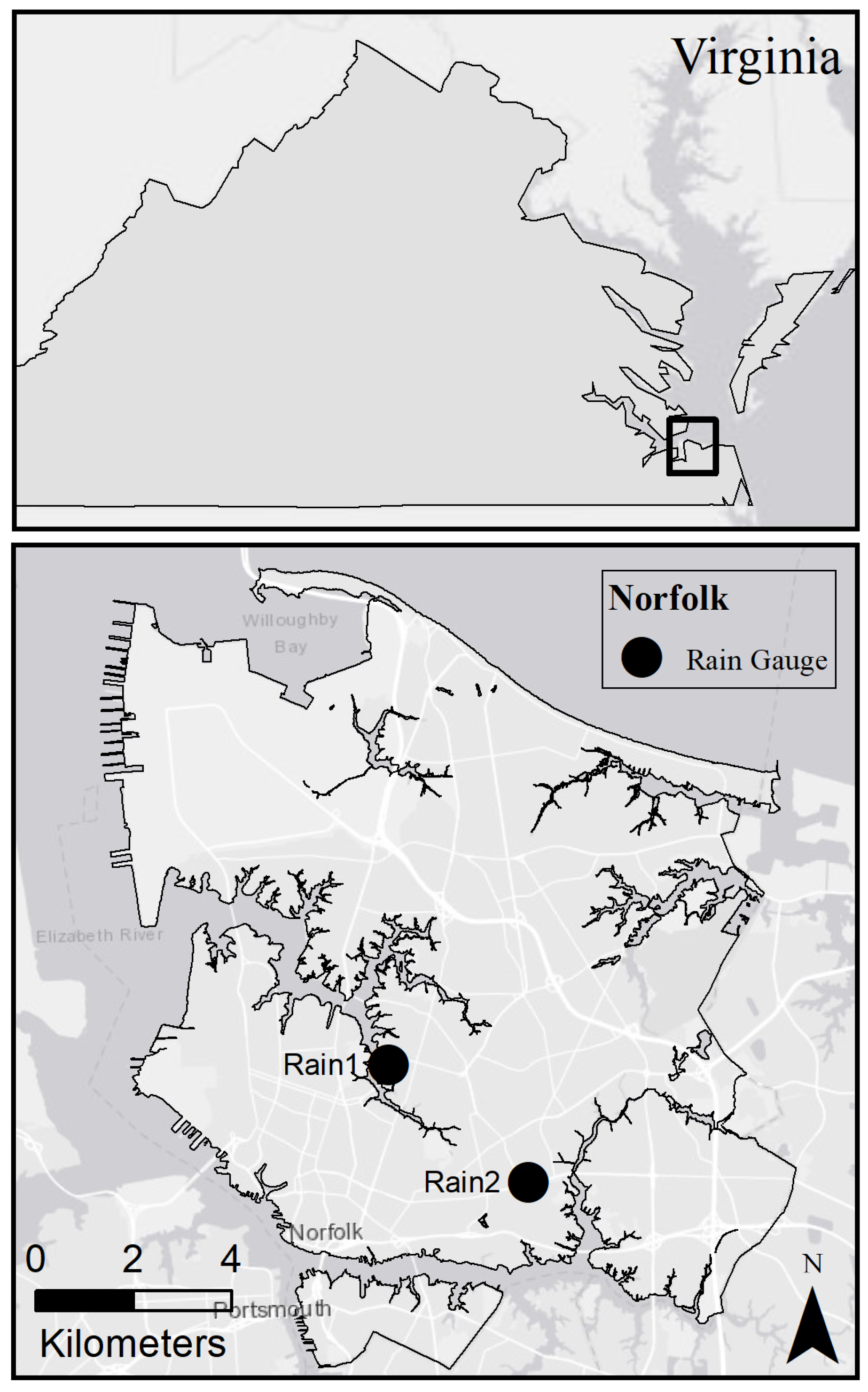
For experimentation, a rainfall data set was obtained from two gauges operated by the Hampton Roads Sanitation District in Norfolk, Virginia (Figure 3). This data set recorded rainfall in 15-min increments from 2010 to 2019. As this is a generic simulation loosely representing a stormwater system in Norfolk, Virginia, the mean of the two data sets was used to provide a rainfall time series more representative of the larger area. From this data, 100 episodes in 24-h periods were selected that were found to result in flooding using a passive system. This was done in order to reduce variability within the successes of the RL implementation—if the RL agent does not have to make any actions and no flooding occurs, it takes longer for an optimal policy to be found.

2.6. Experimental Design

Training simulations were run 10,000 times, making measures and adjustments on a 15-min basis, with each simulation corresponding to a 24 h period within the data set. Training was repeated with each of the testing conditions. This means that in total, 240,000 h were simulated for each condition, equating to a total of 16,000 15-min periods.

For each condition, the episodes were processed into a simulated perfect forecast, giving the sum of the depth of rainfall received during each period in one-hour increments. In other words, one value was created for each hour to represent the total rainfall for that particular hour. This was done for the current hour of the simulation, ($f_1$), and the next, ($f_2$).

Forecasts were found to have an approximate 40% accuracy within a tertile of variation six days in advance; however, the accuracy greatly increases as the timescale decreases (1 h in advance increases accuracy) [33]. The perfect forecast generated has no imperfections, as such to evaluate more real-world performance, noise is added. Thus to simulate uncertain forecasts, ($f_{1–2}^{\prime }$), a uniform distribution (U) was sampled in order to generate a value between the upper (A) and lower bounds (B) of the accuracy,

$$X\sim U(A,B).$$

(10)

This uncertainty was simulated by the product of the perfect forecast and sampled value (X) with upper and lower bounds of 0.95 and 1.05 to create a possible spread of values in between +/−5%.

$$f_1^{\prime }=f_1\times X\sim U(0.95,1.05)$$

(11)

The bounds of the sample became greater the further the forecast was from the current timestep; an example being +/−10% two hours in the future.

$$f_2^{\prime }=f_2\times X\sim U(0.90,1.10)$$

(12)

During the same time period, the SWMM tool simulated water heights and flooding at each node.

For the perfect state data, the exact sensor and exact forecast data were used. For both the uncertain state and uncertain forecast data, the uniform sampling discussed above was utilized; however, additionally, a uniform distribution was again sampled +/−10% for the state data to create the uncertain state condition.

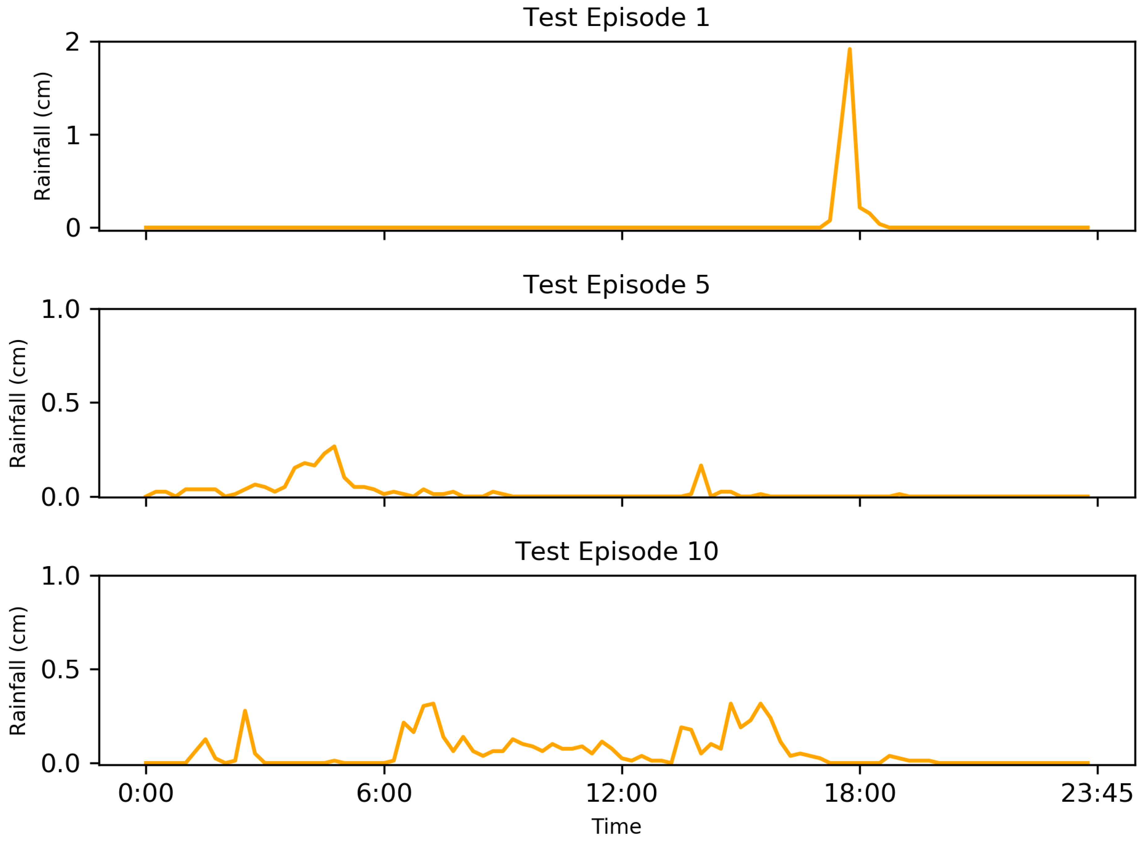
A random sample of 15% of rain events was selected for test episodes (rainfall test episodes 1–15) to compare the performance of each trained RL to that of the passive condition. These test episodes were not used for training to prevent and test for overfitting—the policy is only optimal for the training data. The passive condition mimicked the traditional stormwater systems which are commonly used, and served as a control condition for the RL implementations.

3. Results

3.1. Overall Comparison of RL Agents and Passive System

The performance of each DDPG implementation with perfect and noisy forecast and state information was evaluated against the passive system for the 15 randomly chosen test datasets (Table 2). The table lists the total flooding volume for each episode. Each implementation showed major reductions in overall flooding volume compared to the passive system (Figure 4). When compared to the passive system, total flood volumes had average reductions of 69.23%, 67.90%, and 73.02% for the RL implementations using perfect data, noisy forecast data, and noisy state data, respectively. The episodes 1, 5, and 10 were randomly selected to further explore the performance of the implementations on a step basis.

3.2. Analysis of RL Agent Policies

Of the 15 test rainfall events used to evaluate the performance of the RL implementation, three events—1, 5, and 10—were randomly selected as a sample for further analysis. The rain events for testing episodes one, five, and ten are displayed in Figure 5.

For test episode 1 (Figure 6), where there was approximately 2 cm of rainfall within a 15 min period, all stormwater implementations were quickly overwhelmed. The passive system resulting in $9\times {10}^6{\mathrm{m}}^3$ of flooding, performed the worst. As all of the valves are open, $J_1$ and $J_2$ do not see substantial volume; however, $J_3$ is quickly overwhelmed resulting in the large flooding amounts. The RL implementation using perfect data was able to modulate the valves, resulting in a 32% reduction. Opposed to the passive system, the perfect RL caused flooding at $J_1$ and $J_2$ while keeping $J_3$ below flood stage. In a real-world context, while still causing flooding, it would result in less damage distributing the flood volume across two different areas as opposed to $9\times {10}^6{\mathrm{m}}^3$ at one. Both of the noisy data variants performed similarly resulting in a 50+% reduction. Similar to the perfect data implementation, both kept $J_3$ below flood stage, but they achieved this—noisy state especially—by rapidly cycling the orifices from 0–100%. In a simulated environment, this may be optimal, but in a real-world context, this may not be a desirable behavior. Further research, potentially with another reward function, would be needed to avoid this behavior.

For test episode 5 (Figure 7), there was peak rainfall of approximately 0.4 cm of rainfall over a 15 min period, however there was a continuous, yet minor rainfall for 24 h period. While a seemingly small quantity of water, multiplied across the area of eight subcatchments, the perfect implementation was overwhelmed. Similar to the first episode, $J_{1–2}$ were well below flood stage; however, $J_3$ flooded. In the case of this episode, flooding occurred for nearly 12 of the 24 h resulting in $6\times {10}^6{\mathrm{m}}^3$, the passive performing the worst. The perfect data implementation was able to modulate the valves, resulting in a 96% reduction. Similar to the first test episode, the perfect data implementation caused flooding at $J_1$ and $J_2$ while keeping $J_3$ below flood stage; again distributing the flooding volume to two areas. Both of the noisy data variants performed similarly resulting in a 100% reduction. Each case was able to keep each junction below flood stage.

For test episode 10 (Figure 8), there was a moderate intensity storm peaking at 0.3 cm per 15 min. The storm fluctuated around that volume for the duration of the 24 h. The passive system resulting in over $23\times {10}^6{\mathrm{m}}^3$ of flooding, performed the worst. All junctions had flooding, $J_3$ the most. Opposed to the other test episodes, all of the RL implementations resulted in flooding. The junctions are all overwhelmed in a similar way, yet minor differences result in differences in flooding volume. The perfect data implementation preforms the worst with a 16% reduction, and the imperfect state resulting in a 25% reduction, a range of 9%.

4. Discussion

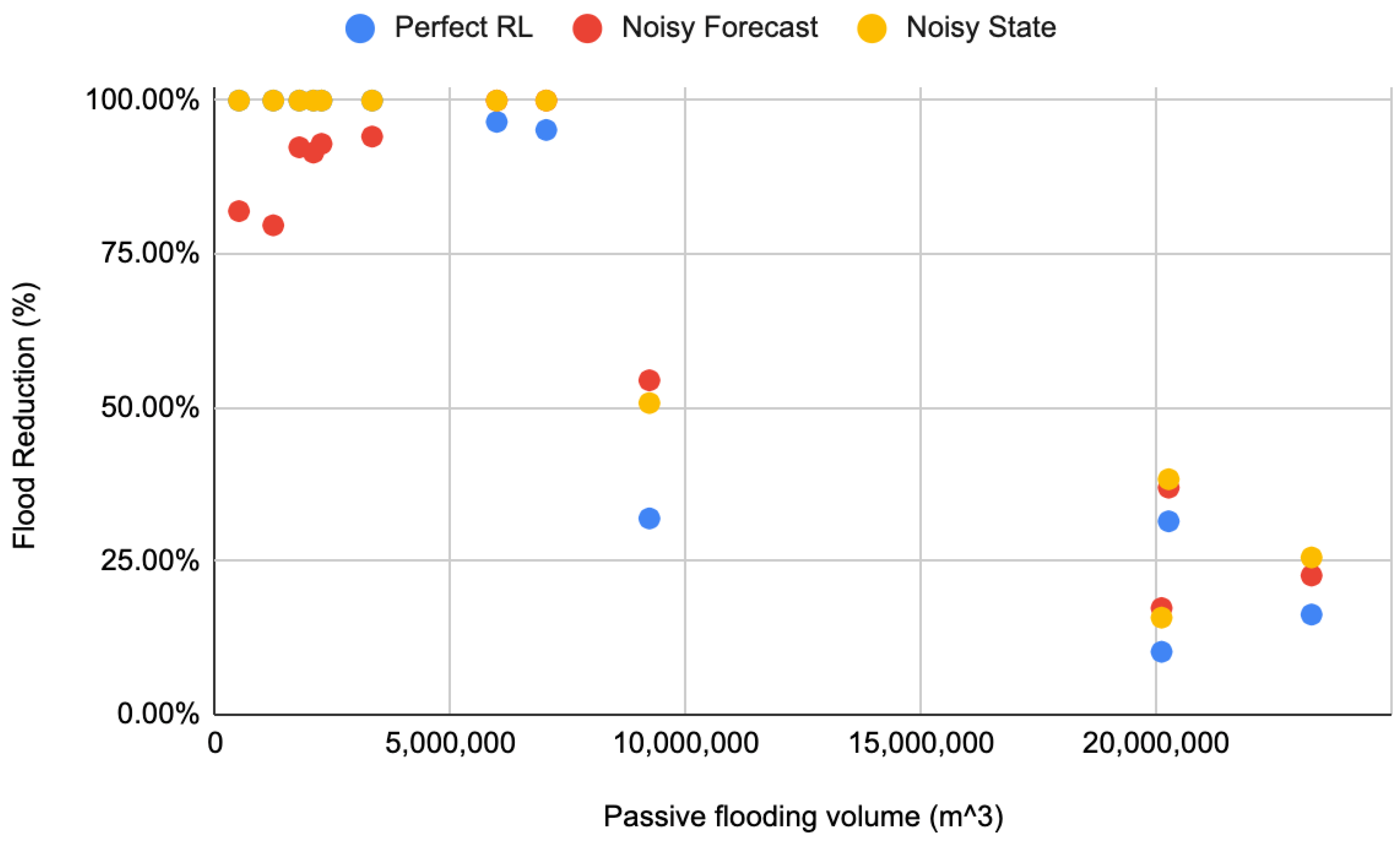
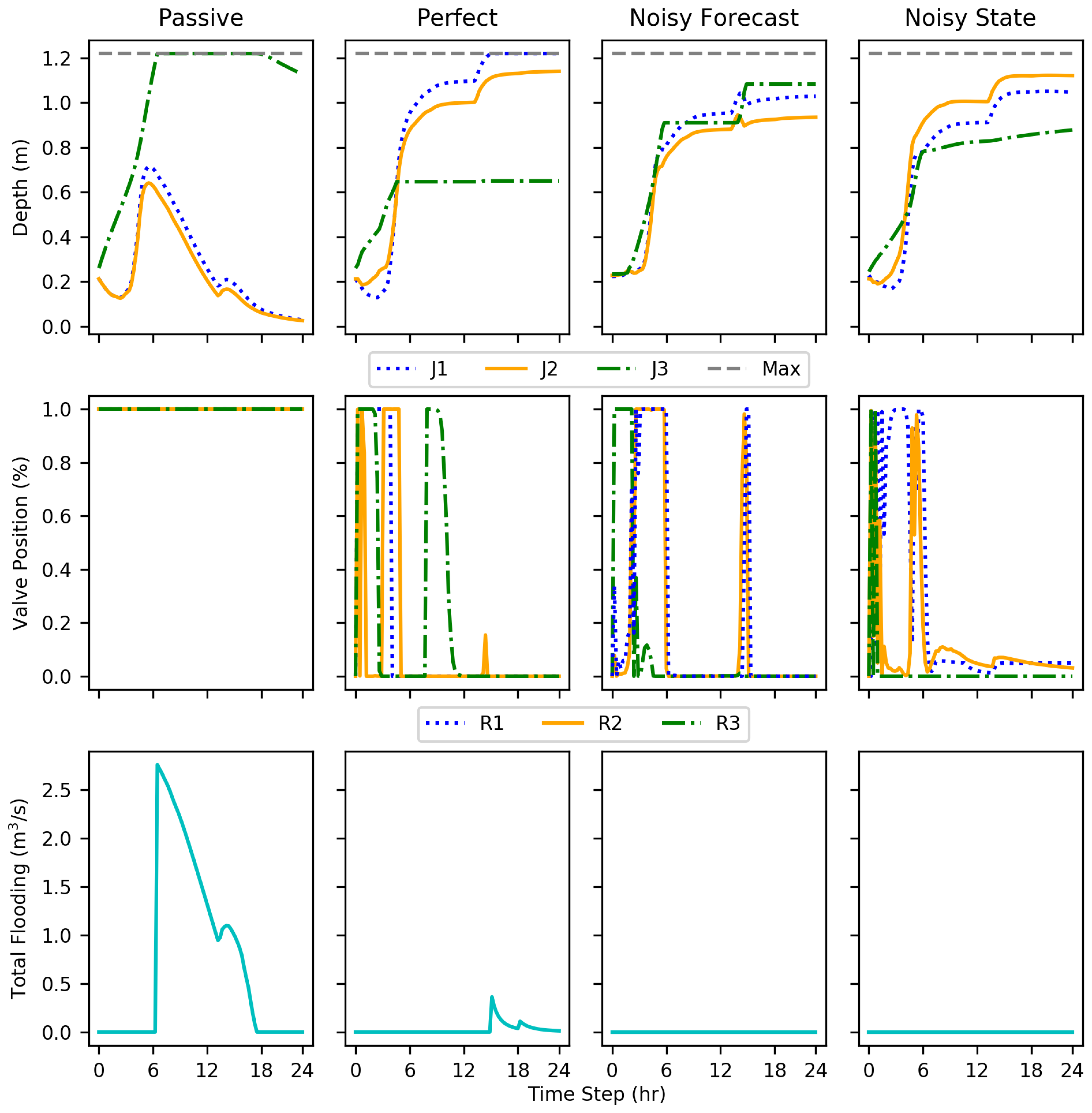
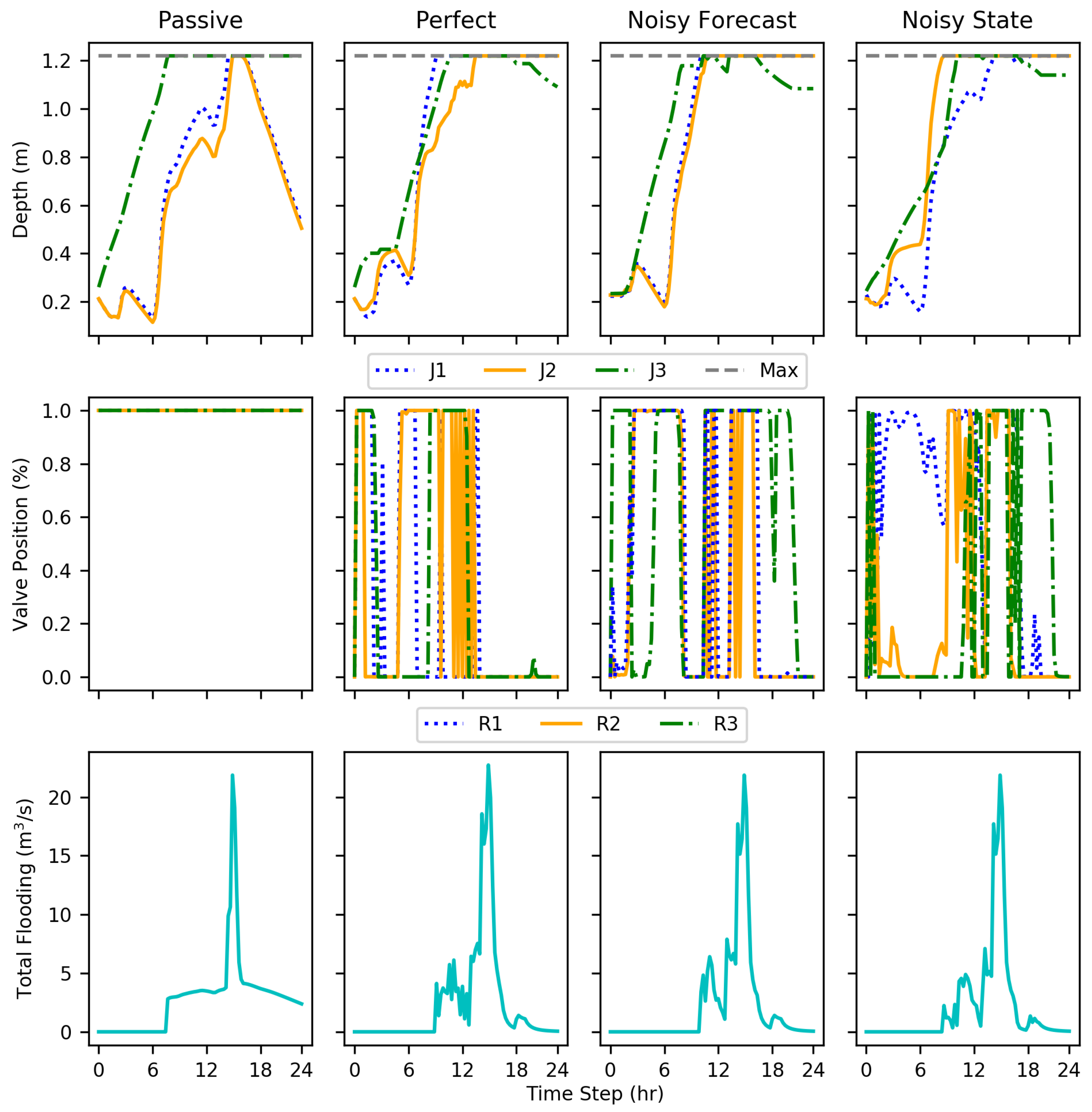
The DDPG implementations, even with added noise, showed reductions in flooding compared to the passive conditions, evaluated on 15 test conditions. The tests show that DDPG learned a policy that reduced total flood volume by an average of 69–73% compared to the passive system and several test events had 100% reductions. The implementations were evaluated using disadvantages more realistic in real-world conditions such as uncertain forecast and state data. Nevertheless, each DDPG implementation performed similarly to the others. This shows the ability to account for and even learn how to use data formerly unused due to unpredictability and uncertainty, such as forecasting.

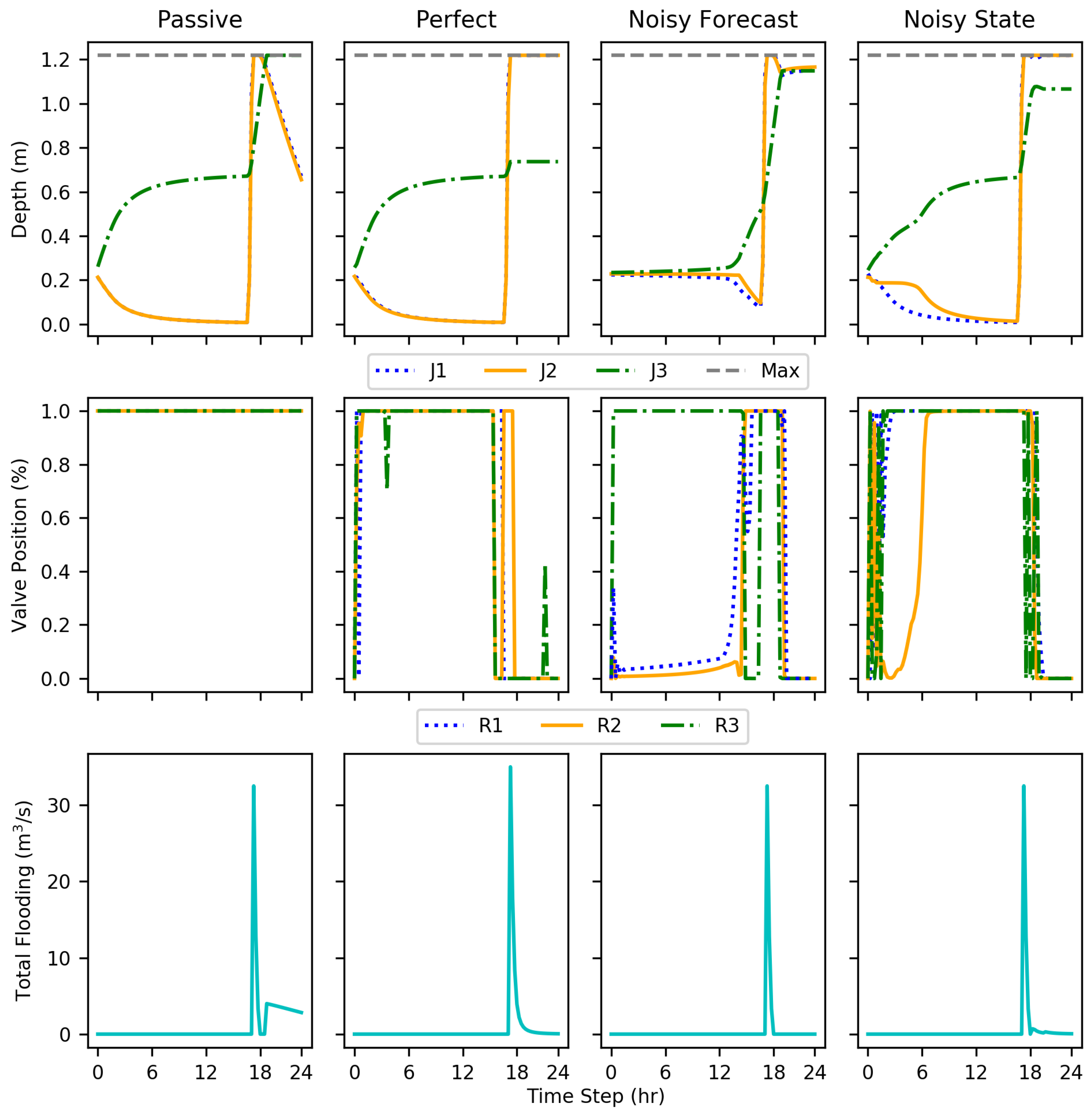
Within the results, each implementation at some point showed rapid cycling between valve positions; this is particularly evident with test episode 10 (Figure 8). This action may be indicative of incomplete training, a fully optimal policy not being completely realized.

While only resulting in an average decrease in flooding volume by an additional one percent, the noisy state implementation performed better than the perfect condition. Without more extensive testing, any explanation may be speculation, but, the better performance can most likely be attributed to further exploration of the state space due to increased irregularity with the state information. Another explanation for the irregularity is simply variation within training. While ideally an optimal policy can be learned every time, there is an aspect of random exploration to RL.

This project acted as a first step showing that DDPG can perform optimally even with uncertain data. However, for an implementation such as this to be utilized in the real world, there are still a multitude of factors that need further exploration, such as the consequences of control system or sensor failure. While uncertain data are more representative of reality and can often lead to unpredictability within a system, the loss or removal of data can have even graver consequences. If a human were to look at operating levels of something such as a storage pond, the human could realize highly improbable values such as a depth of zero, but a machine without vast training on a wide array of issues may never realize there is an error. RL or DDPG solutions are currently limited by what can be simulated. Without the knowledge of what can fail and how, one can only speculate as to the ramifications of a system continuously flooding a storage pond as it thinks it is below standard operating height due to sensor failure.

Reinforcement learning is an evolving field, and computer systems are able to handle larger datasets. A multitude of factors go into the performance of a reinforcement learning implementation, DDPG being no exception [19]. This study utilized a reward function selected following pilot testing of 5 others, each using different methods of administering a negative reward. Other formulae may have produced less total flooding volume, but potentially may be catastrophic based on the concentration of where the flooding occurred. However, without further area specific evaluation; this remains speculation. The reward function chosen for further training and testing would mitigate flooding, but it may have unforeseen consequences based on the current infrastructure model. Additional training cycles would likely improve the results.

The reported rainfall amounts and subsequent flooding, although simulated, were representative of historical events in Norfolk, Virginia. Norfolk has been especially affected by changing weather patterns and climate change due to a rising sea level and development in various surrounding areas. In cases where seawater rises impact stormwater outlets, even minor rain events can lead to so-called nuisance floods [34]. DDPG with the tested reward function, regardless of noise added showed the greatest reduction in flooding during these minor rainfall events, situations when nuisance floods would occur. Thus, communities such as Norfolk could benefit greatly from RL solutions. The SWMM tool helps with the design factors, but the ability to learn how to best adjust the valves during rain events could continually improve.

RL application to mitigate flooding in coastal cities is an emerging strategy for this important problem. Using authentic data sets, with the introduction of noise provides a realistic simulation of stormwater systems. DDPG was able to accommodate a complex model considering an integration of rain forecasting, each with imperfect or noisy data. DDPG and simulations can be adapted with different rainfall datasets and models indicative of other cities and as development of infrastructure continues. Thus, one could relatively quickly retrain the algorithm based on the new environment, and hope to see similar results. The application of DDPG, and, to a greater extent reinforcement learning, has application in a wide variety of civil infrastructure systems, not limited to just stormwater infrastructure. Using DDPG and other machine learning strategies to control critical infrastructure has the ability to process multiple, simultaneous factors in near real-time following sufficient training. Furthermore, this paper describes the ability of the machine to accommodate uncertainties that represent real-world factors and can reduce the loss of life and property by dynamically automating stormwater systems.

5. Conclusions

This study demonstrated the viability and success of a DDPG RL implementation in controlling stormwater systems with a reduction of flooding in a variety of storm events observed in Norfolk, VA. Three stormwater control conditions were compared with the passive system: (i) RL using perfect input data, (ii) RL using noisy forecasts, and (iii) RL using noisy state data. We hypothesized that RL would provide better flood mitigation than the passive system by accommodating for noisy forecast or state data that is more representative of the real-world than having perfect knowledge of current and future states. Three DDPG agents were trained by interacting with a SWMM simulation for 10,000 time steps. Following training, the RL policies were tested on a set of previously unseen rainfall events. We found that the DDPG strategies were able to accommodate uncertain data resulting in similar flood mitigation ability between the three data conditions. Compared to the passive system, the three RL implementations reduced flooding by an average of 70.5% on the test events.

The results of this research demonstrate the promise of using RL to control stormwater systems in real-time, even under uncertain conditions. Additional work to further understand how RL performs for stormwater RTC includes using real rainfall forecasts that are longer than the forecasts used here. This would allow control decisions to be made even further in advance of storm events to prepare the system to prevent flooding. Longer forecasts; however, may include more uncertainty and increase the chance of making inappropriate control decisions. Another key topic to advance this research is to explore RL’s ability to maintain overall system performance when a sensor or group of sensors is not functioning or is reporting erroneous data. This will be especially critical as both the density of sensor networks and the adoption of stormwater RTC systems continue to increase [12].