Evaluating Efficiency Improvement of Deep-Cut Curb Inlets for Road-Bioretention Stripes

Abstract

Making a deep cut on the curb inlet has been used in some sponge-city (SPC) projects for road-bioretention stripes to manage stormwater runoff since they were easily implemented in the field. The efficiencies of the deep-cut curb inlets in those projects were unknown for lacking equation to evaluate their efficiencies. Two kinds of retrofit scenarios are commonly used: (1) The curb-cut cases when the deep cut is made only over the width of the curb inlet; (2) the road-curb cut cases when both the curb inlet and a small part of the road surface have a deep cut. An updated two-dimensional flow simulation program, FullSWOF-ZG, was used to determine two important parameters in road curb inlet design: The 100% interception curb inlet lengths (L_T) and the curb inlet efficiencies (E_ci). Eight-hundred retrofit modeling cases were compared with the no-cut cases to quantify the efficiency improvement of the deep-cut curb inlets. The simulation results show both L_T and E_ci of the curb-cut cases do not improve much. This case study with limited combinations of longitudinal and cross slopes and inlet lengths demonstrated that E_ci of the road-curb cut cases improves to a large extent so that they can be used in the SPC projects and other urban drainage projects to reduce the flooding potentials. A general equation used to design and evaluate the road-curb cut inlets can be developed based on more simulation cases with a wide range of input parameters in a future study.

1. Introduction

Curb inlets are important drainage components for urban stormwater management to traditionally intercept the surface runoff into underground stormwater pipelines or to capture runoff into road-bioretention stripes for infiltration and water quality improvement in many recent designs (Figure 1). The hydraulic performance of undepressed curb inlets (Figure 1b) for roadway drainage has been studied for more than 60 years, which was reviewed and summarized by Izzard [1], Li [2], and systematically documented in the Hydraulic Engineering Circular No. 22 (HEC-22) by Brown et al. [3]. In HEC-22, there are two steps to design curb inlet: (1) Calculate the 100% interception curb inlet length (L_T, the curb-opening length when all upstream inflow is intercepted by the curb inlet) based on road longitudinal slope (S₀), cross slope (S_x), and roughness; (2) calculate the curb inlet efficiency (E_ci, the curb inlet intercepted flow divide by the total inflow from the upstream boundary) based on curb inlet length (L_ci) and L_T.

The undepressed curb inlets have one cross slope for the road surface including the gutter and the curb inlet (Figure 1b). The deep-cut curb inlets (Figure 1c,d) by cutting/deepening curb inlet, were used in some of the retrofit sponge city (SPC) projects for that they were easily implemented based on engineer’s or designer’s field experience. The implementation of the deep cuts was based on some field observations that the undepressed curb inlets could not effectively intercept the runoff from the road surface into the bioretention strip along roads. To improve the interception efficiency, the undepressed curb inlet was retrofitted by simply cutting the curb inlet deeper to create a local depression, for example, making the curb inlet opening area to be 0.10–0.15 m lower than the original surface (Figure 1c). This is the first type of deep-cut curb inlets, called “curb-cut inlet” in this study (or when w₂ = w₁ in Figure 1a). The second type of deep-cut curb inlets is called “road-curb cut inlet” when an undepressed curb inlet was retrofitted by cutting curb inlet and a small part of the road deeper to create a wider local depression (Figure 1d) when w₂ > w₁ in Figure 1a. The efficiencies of both types of deep-cut curb inlets in those projects were unknown because there is no standard equation that can be used to calculate their efficiencies.

To determine inlet efficiency and performance, the reduced-scale physical models were used in some studies and based on Froude number scaling, for example, a 3:4 scale model for Hammonds and Holley’s study [4], 1:4 for Uyumaz’s research [5], and 1:3 for Guo and Mackenzie’s tests [6]. Only Schalla et al. [7] conducted full-scale experiments for the curb inlet. Fang et al. [8] used a three-dimensional computational fluid dynamics (CFD) software, Flow-3D, to develop the numerical models simulating unsteady, free-surface, shallow flow through local depressed curb-opening inlets. They demonstrated that an advanced CFD model could be used as a virtual laboratory to evaluate the performance of curb inlets with different geometry and inflow conditions. In this study, full-scale numerical models were built up and simulated with two-dimensional (2D) FullSWOF-ZG (Li et al. 2019), which fully (Full) solves shallow water (SW) equations for overland flow (OF) and includes submodules modeling infiltration by zones (Z) and flow interception by grate-inlet (G), to study the hydraulic performance of curb inlets.

Compared to undepressed curb inlets, the deep-cut curb inlets at the gutter may have a larger interception capacity for the road-bioretention strips [3]. However, the performance of the curb inlets with two types of deep cuts (Figure 1c,d) was still not quantified in previous studies. This study aims to help more engineers and designers to perform the curb inlet hydraulic design rather than only design it from a landscape perspective for road-bioretention strips since we can quantify the performance improvement of the deep-cut inlets based on two-dimensional overland flow simulation results. Using the FullSWOF-ZG program, it is possible to quantify efficiencies of different types of curb inlets with hundreds of model parameter combinations. These results provide useful information on the design and retrofit of curb inlets for the road-bioretention strips and to determine whether and how the deep-cut should be implemented.

2. Materials and Methods

2.1. Overland flow Simulation Model and Verification Cases

The FullSWOF-ZG was used in this study to simulate the two-dimensional overland flow on the road surface and developed from FullSWOF_2D (version 1.07, Lab. J. A. Dieudonné & EPU Nice Sophia, Nice, France) [9]. The submodules for determining infiltration by zones (pervious and impervious zones in the simulation domain) and grate-inlet drainage from the 2D surface to the 1D pipe were added to the open-source FullSWOF_2D program. FullSWOF_2D fully solves the shallow-water equations (SWEs) for overland flow in two dimensions, which is programmed using C++ to describe the rainfall-runoff and flow distribution progress on the surface in 2D domains [10]. Therefore, the FullSWOF-ZG program can simulate impervious and pervious surfaces (different infiltration parameters or capabilities in different zones) simultaneously under rainfall events. The 2D-1D grate-inlet drainage submodule enables the program to simulate the 2D overland runoff flowing into a grate inlet then to a 1D underground drainage pipe using the weir equation [11]. The model was tested and validated in the previous studies [12,13,14] by comparing it with the collected experimental data.

The two-dimensional SWEs for the FullSWOF_2D program, including the continuity equation and two momentum equations in the x- and y- directions, is stated as the following equations for each computational cell (center coordinates x and y):

$$\frac{\partial h}{\partial t}+\frac{\partial hu}{\partial x}+\frac{\partial hv}{\partial y}=R_i\left(x,y\right)-f\left(x,y\right)$$

(1)

$$\frac{\partial hu}{\partial t}+\frac{\partial }{\partial x}\left(h{u}^2+\frac{g{h}^2}{2}\right)+\frac{\partial }{\partial y}\left(huv\right)=-gh\left(\frac{\partial z}{\partial x}+S_{fx}\right)$$

(2)

$$\frac{\partial hv}{\partial t}+\frac{\partial }{\partial x}\left(huv\right)+\frac{\partial }{\partial y}\left(h{v}^2+\frac{g{h}^2}{2}\right)=-gh\left(\frac{\partial z}{\partial y}+ S_{fy}\right)$$

(3)

where R_i (x, y) (m/s) is the cell’s rainfall intensity; f (x, y) (m/s) is the cell’s infiltration rate; h (m) is the cell’s water depth; z (m) is the cell topography elevation as a function of the cell location or x- and y- coordinates; u (m/s) and v (m/s) are the cell’s depth-averaged velocities in the x- and y- directions, respectively; S_fx and S_fy are the cell’s friction slopes in the x- and y- directions, respectively; g (m/s²) is the gravity acceleration; and t (s) is time.

The FullSWOF_2D program fully solves SWEs on a structured mesh (square cells) in two dimensions using the finite volume method that ensures mass conservation compared to the finite difference method [15]. A well-balanced numerical scheme was adopted to guarantee the positivity of water depth and the preservation of steady states for specific hydrological features such as during wet-dry transitions and tiny water depths [9,16]. A modified bi-layer (crust- and soil-layer) Green–Ampt infiltration model [17] to calculate f(x, y) for Equation (1) was added in the FullSWOF_2D [15], which enables the program to simulate the overland flow on impervious and pervious surfaces simultaneously.

FullSWOF_2D was tested against the data from undepressed curb inlet cases in Spaliviero’s [18] study; local depressed curb inlet cases conducted by Hammonds and Holley [4]; and overland flow on previous surface cases observed by Esteves et al. [17]. The differences of simulated and observed curb inlet interception efficiencies (∆E) ranged from −3.7% to 4.4% with an average $\pm$ standard deviation of 0.8% $\pm$ 2.6% for undepressed curb inlet cases [19]. The percent differences of simulated and observed intercepted efficiencies (PDE) ranged from −4.8% to 18.7% with an average $\pm$ standard deviation of 3.7% $\pm$ 8.3%. The differences, ∆E ranged from −3.2% to 13.2%, with an average $\pm$ standard deviation of 3.5 $\pm$ 3.5% for local depressed curb inlet cases. The percent differences, PDE of the simulated and observed intercepted efficiencies ranged from −6.0% to 28.7%, with an average $\pm$ standard deviation of 6.6 $\pm$ 7.3% [12]. In a previous study by Fang et al. [8], the differences ∆E ranged from −7.0% to 17.6%, with an average $\pm$ standard deviation of 1.0 $\pm$ 4.87% in their 3D FLOW-3D simulations for local depressed curb inlet. The percent differences, PDE for Fang’s study ranged from −19.7% to 6.1%, with an average $\pm$ standard deviation of −0.8 $\pm$ 5.7%. These 2D overland flow simulation cases using the FullSWOF-ZG program were almost as good as the FLOW-3D cases used in the previous study when trying to simulate the interception efficiency of the local depressed curb inlet cases under different situations, but the simulation time was much shorter for running 2D FullSWOF-ZG. The Nash–Sutcliffe Efficiency (NSE) coefficient [20] of FullSWOF-ZG and Esteves’s study ranged from 0.64 to 0.95 (average $\pm$ standard deviation as 0.75 $\pm$ 0.11) and from 0.46 to 0.93 (0.79 $\pm$ 0.15) for overland flow on pervious surfaces simulation, respectively [14]. The simulated results for undepressed curb inlet, local depressed curb inlet, and overland flow on previous surface cases were matched well with the observed data, which proves that the FullSWOD-ZG program can not only simulate overland flow on pervious and impervious surfaces accurately, but also predict the curb inlet efficiency very precisely.

2.2. Modeling Cases for the Deep-Cut Curb Inlets

Two types of retrofitted curb inlets were simulated in this study: (1) Curb-cut inlets when the deep cut is made only over the width of the curb inlet (Figure 1b and Figure 2a,b); (2) road-curb cut inlets when both the curb inlet and a small part of road surface have a deep cut (Figure 1c and Figure 2c,d). The curb width or thickness for all modeling cases was set at 0.10 m (10 cm) along the cross-slope direction. Typically, the deep-cut depth d (Figure 1c) could be about 0.05–0.20 m. For the curb-cut inlets, 200 modeling cases with one longitude slope S₀, 10 cross slopes S_x, 10 upstream inflows (Q_in, Figure 2) were used in this study to determine the 100% interception curb inlet lengths, L_T with d = 0.10 m or 0.15 m when the curb or cut width w₁ = 0.10 m. Another 200 modeling cases with the same longitude slope and 10 cross slopes plus 10 curb inlet lengths (L_ci, Figure 1d) were used to determine the curb inlet efficiencies E_ci with d = 0.10 m or 0.15 m. For the road-curb cut inlets, the above-mentioned 400 modeling cases were used to determine either L_T or E_ci with a cut width on the road surface (w₂–w₁) equal to 0.05 m or 0.10 m (Figure 1c) when d is set to 0.1 m. Therefore, a total of 800 modeling cases for the deep-cut curb inlets were designed and modeled using the FullSWOF-ZG program. These cases were compared with the undepressed curb inlet cases to quantify the efficiency improvement for two types of deep-cut curb inlets (Figure 1).

The digital elevation models (DEMs) for the two types of deep-cut curb inlets under different cross slopes and curb inlet lengths were established using MATLAB [21] code. Figure 2 shows examples of the plan view and high-resolution DEMs for four modeling cases with S₀ = 0.01 and S_x = 0.06. Therefore, DEMs of the road surface shown in Figure 2a–d are the same for all four cases, and only DEMs for the inlet and associated cuts on the curb and adjacent road are different and discussed in more detail in Section 2.2.1 and Section 2.2.2. Figure 2a,b is a modeling case for the curb-cut scenarios when the deep cut only occurs over the curb width (0.10 m). Figure 2c,d is a modeling case for the road-curb cut scenarios when the deep cut occurs both over the curb (0.10 m) and a small part of road width (0.05 or 0.10 m).

2.2.1. Determining 100% Interception Curb Inlet Lengths

Figure 2a shows the modeling case to determine L_T for a cut depth d = 0.15 m over the curb inlet. The area in the simulation domain for all modeling cases in this study is 15 m in length (x-direction) and 6.7 m in width (y-direction) that includes 3 m of the car lane, 1.5 m of the bike lane, 2.1 m of the parking lane (1.5 m + 0.6 m gutter), and 0.1 m of the curb. When y = 0, it is the centerline of the road; when y = 6.6–6.7 m, it is the curb. The curb lasts 10 m in the x-direction and there is a long curb-inlet opening (5 m) at x = 10 m (Figure 2a,c) used to determine L_T since the intercepted flow (Q_ci) of a curb inlet is not affected by the downstream curb (i.e., Q_ci = Q_in, bypass flow Q_bp = 0).

The upstream inflow Q_in is set at the left boundary of the simulation domain and flows towards the downstream to the right boundary. The 100% interception curb inlet length L_T is the flow length over the curb inlet determined by the numerical model simulation when Q_ci is equal to Q_in. The intercepted flow is the total flow left the simulation domain from the top boundary determined by the FullSWOF-ZG program. The bypass flow Q_bp is the flow left the simulation domain from the downstream (right) boundary. In the model set up (Figure 2a,d), the curb opening length was 5 m, longer than L_T to be determined so that Q_bp = 0.

All cell elevations in the simulation domain were calculated using a MATLAB program when the bottom-left-corner reference cell’s elevation (the highest in the domain) was assumed to be 10 m. The road surface elevations vary with longitudinal and cross slopes. All cells for the 0.1 m wide curb were set 0.2 m higher than the road surface cells. The cell’s elevations inside the curb inlet were first calculated using the same cross slope of the road surface and then subtracted by the deep cut depth to obtain the final cell’s elevation for the deep cut modeling cases. It was expected to help and allow the runoff to flow into the roadside bioretention. The deep cut inside the curb inlet has a local depression d from the nearby road surface. It is simple and easy to implement when retrofitting curb inlets for the bioretention strip projects to hopefully improve the inlet efficiency.

Two hundred modeling cases were selected and modeled to determine L_T for the combinations of 10 S_x, 10 Q_in (

Table 1. Sequence numbers and corresponding geometry and inflow parameters of curb inlet modeling cases.

Sequence No.	Sx (%)	Modeling Case Index 1	Modeling Case Index 2	Qin (L/s)	Modeling Case Index 3	Modeling Case Index 4	Lci (m)
1	1.5	UDX1Q1	D1X1Q1	6	UDX1L1	D1X1L1	0.15
2	2.0	UDX2Q2	D1X2Q2	8	UDX2L2	D1X2L2	0.30
3	2.5	UDX3Q3	D1X3Q3	10	UDX3L3	D1X3L3	0.45
4	3.0	UDX4Q4	D1X4Q4	12	UDX4L4	D1X4L4	0.60
5	3.5	UDX5Q5	D1X5Q5	14	UDX5L5	D1X5L5	0.75
6	4.0	UDX6Q6	D1X6Q6	16	UDX6L6	D1X6L6	0.90
7	4.5	UDX7Q7	D1X7Q7	18	UDX7L7	D1X7L7	1.05
8	5.0	UDX8Q8	D1X8Q8	20	UDX8L8	D1X8L8	1.20
9	5.5	UDX9Q9	D1X9Q9	22	UDX9L9	D1X9L9	1.35
10	6.0	UDX10Q10	D1X10Q10	24	UDX10L10	D1X10L10	1.50

Note ¹—undepressed modeling case for determining L_T conducted in the previous study [12], ²—modeling case for determining L_T when cut depth d = 0.1 m, ³—undepressed modeling cases for determining E_ci of different L_ci when Q_in = 10 L/s conducted in the previous study [12], ⁴—modeling cases for determining E_ci of different L_ci when Q_in = 10 L/s when d = 0.1 m.

), and two d (0.10 and 0.15 m). The cell size of DEMs for all 200 cases was 0.025 m determined by a sensitivity analysis. The simulated water depth along the curb increases along the x-direction first and then starts to decrease after it reaches the curb inlet (x > 10 m) [12]. The depth limit equal to 0.2 mm was used to determine L_T and already tested and verified in the previous study [12].

Commonly used S₀ and S_x values in stormwater drainage design were chosen from the HEC-22 [3] for 100 modeling cases, which have one longitudinal slope S₀ = 0.01 (1%), 10 cross slopes S_x = 0.015–0.06 (1.5–6%), and 10 upstream inflows Q_in = 6–24 L/s (Table 1). In this case study, the longitudinal slope of 1% was used. In China, many roads were constructed with small longitudinal slopes, and there are also many roads with steep longitudinal slopes over the world. How the deep cut can affect L_T for the roads with other longitudinal slopes is not comprehensively studied here and should be done in a future study. As reported in Pavement and Geometric Design Criteria for Minimizing Hydroplaning, a cross slope of 2% has little effect on driver effort in steering or on friction demand for vehicle stability. The use of a cross slope steeper than 2% on pavements with a central crown line is not desirable [22]. In areas of intense rainfall, a somewhat steeper cross slope (2.5%) may be used to facilitate drainage as HEC-22 [3] states.

The first 100 modeling cases have a cut depth d of 0.10 m and the second 100 modeling cases having d = 0.15 m. The case number was named using the sequence number (1–10) of the parameter’s choice of S_x and Q_in. For example, the modeling case D1X1Q1 means the road having S₀ = 0.01 (1%), a cut depth d = 0.10 m, S_x = 0.015 (1.5%) with Q_in = 6 L/s for upstream inflow. The modeling case D2X1Q1 has a cut depth d = 0.15 m with the same S₀, S_x, and Q_in for the D1X1Q1 case.

2.2.2. Evaluating the Curb Inlet Efficiency

To evaluate the curb inlet efficiency at different inlet lengths (Figure 2b), the second 200 modeling cases were selected: 10 choices of L_ci, 2 cut depths d (0.10 and 0.15 m), and the same 10 choices for S_x, which were used for the modeling cases to determine L_T. Ten curb inlet opening lengths L_ci that range from 0.15 to 1.5 m with an increase of 0.15 m were adapted based on the curb inlet survey conducted by Stoolmiller et al. [23]. The imposed upstream inflow Q_in was chosen as 10 L/s for the left boundary condition of the domain for the second 200 modeling cases. A part of the inflow is intercepted by the curb inlet, i.e., Q_ci, and the remainder of the inflow is discharged or bypassed downstream along the road, i.e., Q_bp where the inlet length L_ci is less than L_T for 100% interception. The modeling case D1X1L1 means the road having S₀ = 0.01 (1%), cut depth d = 0.10 m, S_x = 0.015 (1.5%) with L_ci = 0.15 m. Figure 2b shows DEM and model set up for D1X10L10 (d = 0.1 m, L_ci = 1.50 m). An undepressed curb inlet when d = 0 has been simulated in a previous study [12].

2.3. Modeling Cases for the Road-Curb Cut Curb Inlets

2.3.1. Determining 100% Interception Curb Inlet Lengths

Figure 2c shows the plan view and high-resolution DEM for the modeling case with S₀ = 0.01 and S_x = 0.06 for a road-curb cut scenario. The difference for two groups of the road-curb cut cases is the cut width w on the road surface (w = w₂ − w₁) (Figure 1d): 0.05 m or 0.10 m. The road cut width w of Figure 2c is 0.10 m and the cut depth d over the curb and adjacent road is 0.10 m.

In this part of the case study, the cut depth for the curb inlet and road surface was fixed at 0.10 m for all cases with S₀ = 0.01 (1%). The case number was named using the sequence number (1–10) of the parameter’s choice of w, S_x, and Q_in. For example, the modeling case R1X1Q1 means the road having a cut width w = 0.05 m, S_x = 0.015 (1.5%), and Q_in = 6 L/s for upstream inflow. Ten R1XmQm (m = 1, 2, …, 10) modeling cases and parameters are listed in

Table 2. Sequence numbers and corresponding geometry and inflow parameters of road-curb cut inlet modeling cases

Sequence No.	Sx (%)	Modeling Case Index 1	Qin (L/s)	Modeling Case Index 2	Lci (m)
1	1.5	R1X1Q1	6	R1X1L1	0.15
2	2.0	R1X2Q2	8	R1X2L2	0.30
3	2.5	R1X3Q3	10	R1X3L3	0.45
4	3.0	R1X4Q4	12	R1X4L4	0.60
5	3.5	R1X5Q5	14	R1X5L5	0.75
6	4.0	R1X6Q6	16	R1X6L6	0.90
7	4.5	R1X7Q7	18	R1X7L7	1.05
8	5.0	R1X8Q8	20	R1X8L8	1.20
9	5.5	R1X9Q9	22	R1X9L9	1.35
10	6.0	R1X10Q10	24	R1X10L10	1.50

Note ¹—modeling case for determining L_T with cut depth d = 0.10 m, ²—modeling cases for determining E_ci of different lengths L_ci when Q_in = 10 L/s.

. The 100 modeling cases R2XmQn (m or n = 1, 2, …, 10) mean the road has a cut width w = 0.10 m. The curb opening length (5 m) was set large enough to intercept 100% inflow for these third 200 modeling cases.

2.3.2. Evaluating the Curb Inlet Efficiency

To evaluate the curb inlet efficiency at different inlet lengths (Figure 2d) with different cut widths over the road and curb inlet, the fourth 200 modeling cases were selected using 10 choices of L_ci, 2 cut widths w (0.05 and 0.1 m), and the same 10 choices for S_x, which were used for the third 200 modeling cases to determine L_T. Ten curb inlet lengths L_ci were again ranged from 0.15–1.5 m with an increase of 0.15 m [23]. The imposed upstream inflow Q_in was chosen as 10 L/s for the left boundary condition of the domain. The modeling case R1X1L1 means the road has a cut width w = 0.05 m, S_x = 0.015 (1.5%), and L_ci = 0.15 m (Table 2).

3. Results and Discussion

3.1. 100% Interception Curb Inlet Length for the Curb-Cut and Road-Curb Cut Scenarios

Figure 3 shows the comparison of 100% interception curb inlet length for 100 undepressed cases, 200 curb-cut modeling cases with d = 0.10 m and 0.15 m. The L_T for 100 undepressed cases ranges from 1.91 m to 7.59 m with an average $\pm$ standard deviation equal to 3.69 $\pm$ 1.24 m. The percentage changes of L_T between the curb-cut cases (D1 and D2) and the undepressed cases (UD) with the same S₀, S_x, and Q_in range from −1.09% to 0.00% with the mean percentage change equal to −0.25%. The standard deviation of the percentage changes between the undepressed cases and the curb-cut cases was equal to 0.33%. The 100% interception curb-inlet lengths for the 200 curb-cut cases with different cut depths were quite similar to the L_T for corresponding undepressed cases with the same cross slope and upstream inflow. It means if the deep cut is only made over the curb inlet width, the cut depth (d = 0, 0.05, and 0.10 m) does not make much difference in L_T for S_x = 1.5–6%.

Figure 3 also shows the comparison of 100% interception curb inlet lengths for the undepressed inlets and the road-curb cut inlets with w = 0.05 m and 0.10 m from 100 modeling cases by varying S_x and Q_in. The percentage changes of L_T between the R1 road-curb cut cases with w = 0.05 m and the undepressed cases range from −3.92% to −1.47% with the mean change and its standard deviation of −2.31% and 0.48%. The percentage changes of L_T between the R2 road-curb cut cases with w = 0.1 m and the undepressed cases range from −6.54% to −3.08% with the mean change and its standard deviation of −4.45% and 0.78%. The 100% interception curb inlet length sequence from the largest to smallest was UD > R1 > R2. The maximum reduction of L_T for R1 and R2 cases in comparison to corresponding UD cases is 0.15 and 0.25 m, respectively.

3.2. Curb inlet Efficiency for the Curb-Cut Scenarios

Figure 4 shows the comparison of simulated curb inlet efficiencies for 100 undepressed modeling cases, 200 curb-cut modeling cases with d = 0.10 m and 0.15 m. The inlet efficiencies for the undepressed curbs range from 4.68% to 94.47% with an average $\pm$ standard deviation equal to 43.68% $\pm$ 25.04% when L_ci varied from 0.15 to 1.5 m. The inlet efficiencies for the D1 and D2 curbs range from 5.67% to 94.85% with an average $\pm$ standard deviation equal to 46.06% $\pm$ 24.62%. Simulated curb inlet efficiencies are the same for d = 0.1 m and 0.15 m when other parameters (S₀, S_x, and L_ci) are the same. The percent changes of the curb inlet efficiencies between the curb-cut cases (D1 and D2) and the undepressed cases (UD) range from 0.41% to 26.92% with the mean percentage change of 8.91% and the standard deviation of 6.87%. Figure 4 shows a slight difference between the undepressed and curb-cut cases when E_ci between 0.2 and 0.6. The E_ci changes between the curb-cut cases (D1 and D2) and the undepressed cases (UD) range from 0.39% to 6.01% and are greater than zero so that the curb-cut inlets only increase E_ci a few percent.

Figure 3 and Figure 4 show that the differences in modeling cases between the curb-cut and undepressed curb inlets are very small in terms of the 100% interception curb inlet length and the inlet efficiency. Therefore, it is not an efficient method to improve the curb inlet efficiency only by cutting the curb inlet because E_ci only increases by 0.39–6.01%. The change of cut depth from 0.10 to 0.15 m has almost no influence on the 100% interception curb inlet length and the curb inlet efficiency based on the simulation results.

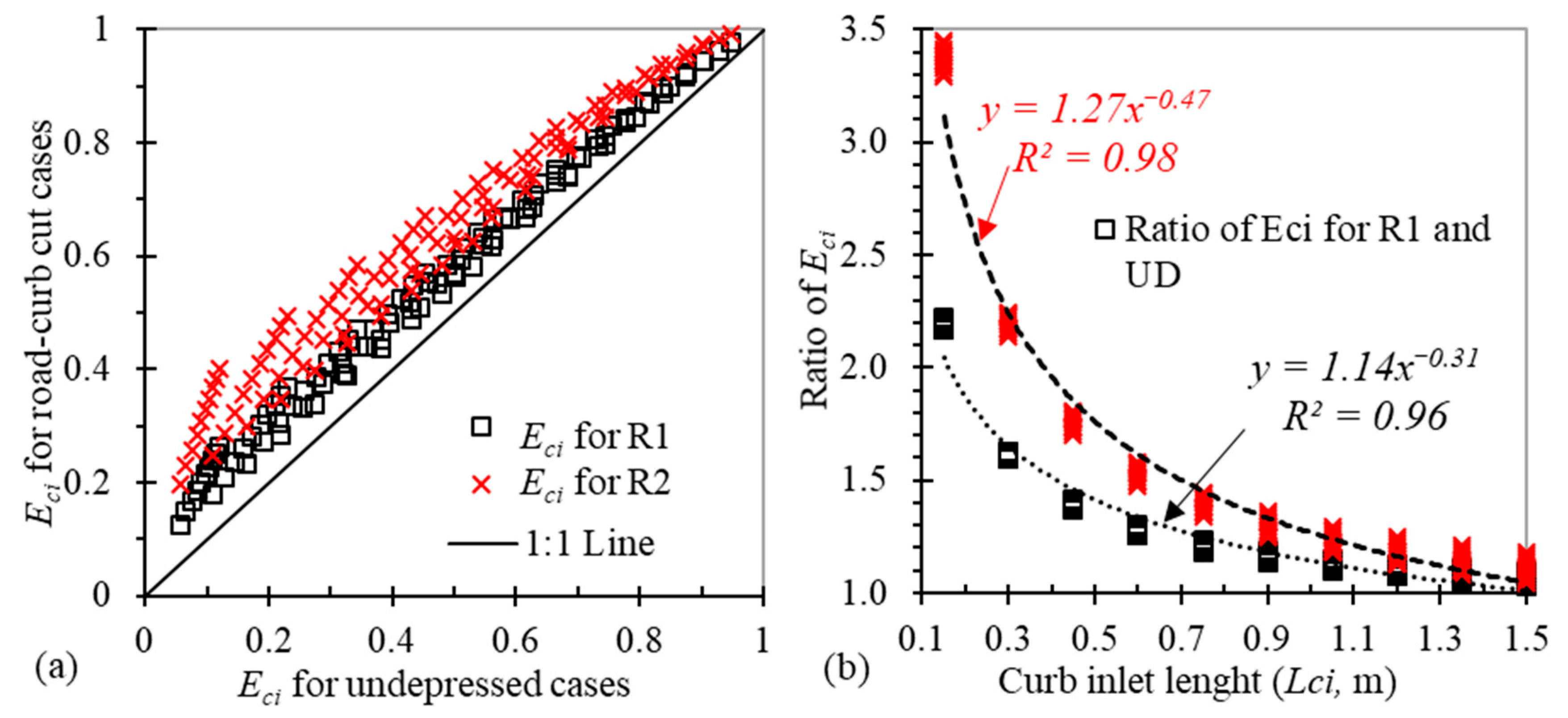
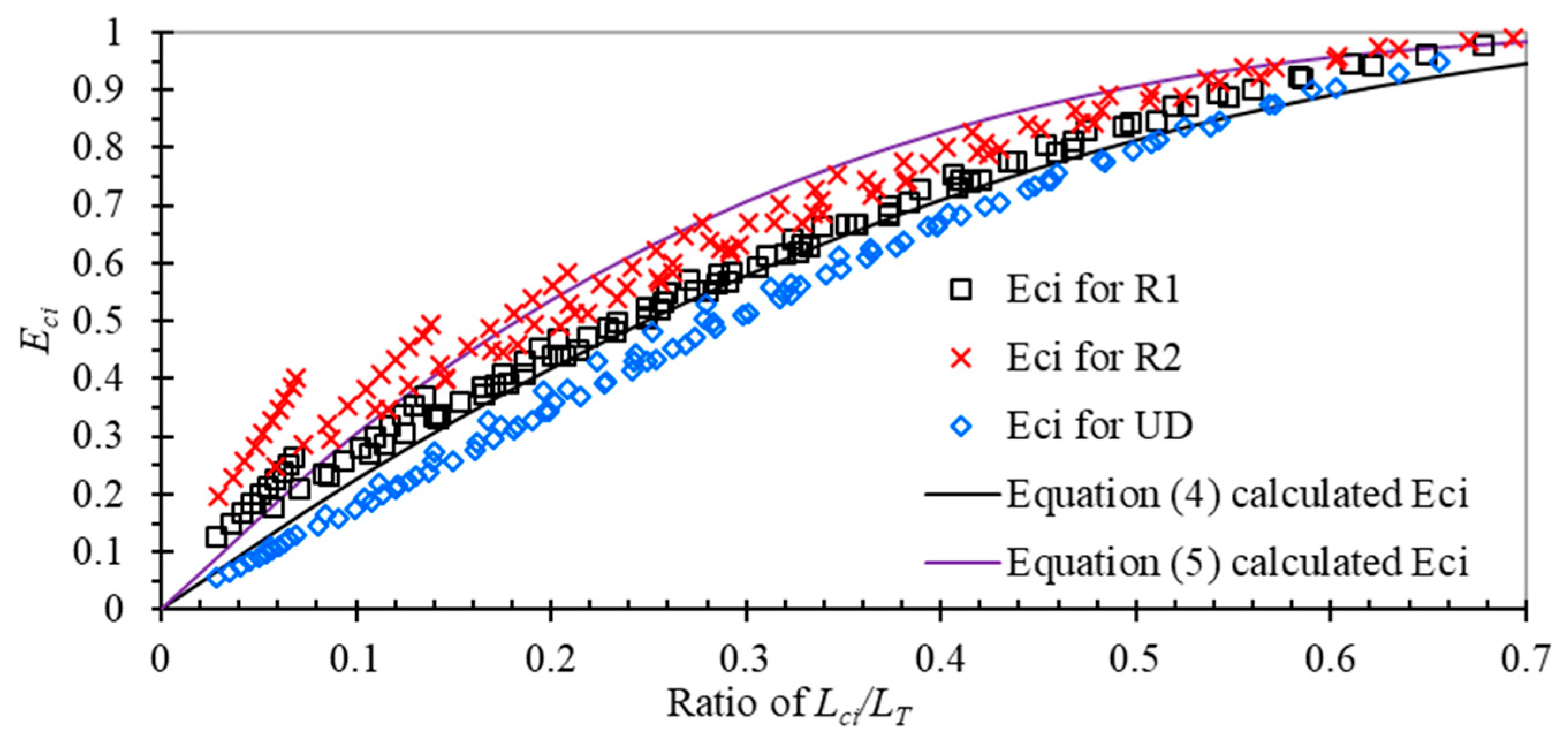
3.3. Curb inlet Efficiencies Evaluation for the Road-Curb Cut Scenarios

Figure 5a shows the comparison of curb inlet efficiency for undepressed (UD) cases, road-curb cut cases with w = 0.05 m (R1 cases) and 0.10 m (R2 cases). The change of curb inlet efficiency between the R1 road-curb cut cases and undepressed cases ranges from 2.79% to 14.16% with the average $\pm$ standard deviation equal to 8.21 $\pm$ 2.55%. The percentage changes of curb inlet efficiency between the R2 road-curb cut cases and undepressed cases range from 4.29% to 27.88% with the average $\pm$ standard deviation equal to 15.63 $\pm$ 5.16%.

Figure 5b plots the ratio of curb inlet efficiency between the road-curb cut cases and corresponding undepressed cases versus the curb inlet length. It is clearly shown that the curb inlet efficiency was largely improved for small curb inlet length. For bioretention facilities in Sponge City projects, many curb inlets have short opening lengths. When L_ci is 0.15 m and 0.3 m, the curb inlet efficiency is average 2.19 and 3.37 times of E_ci for undepressed inlets, respectively, when Q_in = 10 L/s. The road cut width w increases from 0.05 m (R1) to 0.10 m (R2), E_ci for R2 is 1.0–1.55 times of E_ci for R1. Figure 6 shows the curb inlet efficiency E_ci for the undepressed cases, the road-curb cut cases with w = 0.05 m and 0.10 m versus the ratio of L_ci/L_T. The dark line in Figure 6 shows the calculated efficiencies using the equation developed in a previous study [12].

$$E_{ci}=1-{\left[1-\left(\frac{L_{ci}}{L_T}\right)\right]}^{2.42}$$

(4)

where E_ci is the curb inlet efficiency with different curb inlet length, L_ci is the curb inlet length, and L_T is the 100% interception curb inlet length.

A new regression equation of E_ci to L_ci/L_T for R2 cases was developed with an RMSE of 6.26% for these simulation cases.

$$E_{ci}=1-{\left[1-\left(\frac{L_{ci}}{L_T}\right)\right]}^{3.44}$$

(5)

Equation (5) was developed only based on those 100 cases with a longitudinal slope equal to 1%. A general equation that can be used to calculate the road-curb cut inlet efficiency with a wide range of parameters for the road surface (S_o, S_x, and Q_in), curb inlet (L_ci), and cut width (w) still needs to be determined based on more simulation cases in a future study.

For Equation (4), the root mean square error (RMSE) between fitted and simulated E_ci is 3.93%. The differences of curb inlet efficiency between the calculated and simulated results for undepressed cases (UD) range from −2.43% to 7.43% with the average $\pm$ standard deviation equal to 4.06 $\pm$ 2.34%. The calculated E_ci is therefore on the average 4.06% larger than the simulated E_ci (Figure 6). Its RMSE is 4.68%, just slightly larger than the RMSE of Equation (5). It shows the calculated results with Equation (5) match reasonably well with the undepressed cases.

The differences of curb inlet efficiency between the calculated and simulated results for the R1 road-curb cut cases range from -10.70% to 0.35% with the average $\pm$ standard deviation equal to −3.25 $\pm$ 2.28%, which is within the RMSE of Equation (4). The percentage change of curb inlet efficiency between the calculated and simulated results for the R2 road-curb cut cases ranges from −24.07% to −4.86% with the average $\pm$ standard deviation equal to −9.79 $\pm$ 4.50%. Therefore, Equation (4) underestimated the curb inlet efficiencies for the road-curb cut cases with w = 0.01 m, and the average difference is more than twice the RMSE of Equation (4).

4. Conclusions

Two kinds of retrofit scenarios for curb inlets were simulated using the FullSWOF_ZG program in this case study: (1) The deep cut is made only over the width (0.01 m) of the curb inlet (D1 and D2 cases); (2) both the curb inlet and a small part of the road surface have a deep cut (R1 and R2 cases). Simulated results of 800 modeling cases were compared with undepressed curb inlet results to explore and quantify the efficiency improvement of the deep-cut curb inlets. The percentage changes of L_T between the curb-cut cases and the undepressed cases (UD) with the same S₀, S_x, and Q_in range from −1.09% to 0.00% with the mean percentage change equal to −0.25%. The L_T for curb-cut cases with different cut depths were quite similar to the L_T for corresponding undepressed cases with the same cross slope and upstream inflow. It means if the deep cut is only made over the curb inlet width, the cut depth (d = 0, 0.05, and 0.10 m) does not make much difference in L_T for S_x = 1.5–6% tested in this study. The E_ci changes between the curb-cut cases and the undepressed cases (UD) range from 0.4% to 6.0% and are greater than zero so that the curb-cut only increases E_ci a few percent. Therefore, it is not an efficient method to improve the curb inlet efficiency only by cutting the curb inlet because E_ci only increases up to 6.0%.

The sequence from the largest to smallest for 100% interception curb inlet length L_T was UD > R1 > R2 cases. The maximum reduction of L_T for R1 and R2 cases in comparison to corresponding UD cases is 0.15 and 0.25 m, respectively. The increases of curb inlet efficiency between the road-curb cut cases R1 or R2 and the undepressed cases range from 2.79% to 14.2% and 4.3% to 27.9%, respectively. The road-curb cut cases improve the curb inlet efficiency to a large extent so that they can be used in the SPC retrofit projects or other urban drainage projects to reduce flooding potentials. This case study used limited combinations of longitudinal slope (1%), 10 cross slopes, 10 upstream inflows, and 10 inlet lengths to derive the above results. Even the relation of E_ci and L_ci/L_T was explored (Equation (5)), however, a general equation used to design and evaluate the road-curb cut inlets should be developed based on more simulation cases with a wide range of input parameters in a future study.

References

1. Izzard, C.F. Tentative results on capacity of curb opening inlets. In Proceedings of the 29th Annual Conference of the Highway Research Board, Washington, DC, USA, 13–16 December 1950; Highway Research Board: Washington, DC, USA, 1950; pp. 11–13. [Google Scholar]
2. Li, W.H. Hydraulic theory for design of stormwater inlets. In Proceedings of the 33rd Annual Meeting of the Highway Research Board, Washington, DC, USA, 12–15 January 1954; Highway Research Board: Washington, DC, USA, 1954; pp. 83–91. [Google Scholar]
3. Brown, S.; Stein, S.; Warner, J. Urban Drainage Design Manual: Hydraulic Engineering Circular No. 22 (FHWA-NHI-10-009, HEC-22); National Highway Institute: Arlington, VA, USA, 2009. [Google Scholar]
4. Hammonds, M.A.; Holley, E. Hydraulic Characteristics of Flush Depressed Curb Inlets and Bridge Deck Drains (FHWA/TX-96/1409-1); Texas Department of Transportation: Austin, TX, USA, 1995.
5. Uyumaz, A. Urban drainage with curb-opening inlets. In Proceedings of the Ninth International Conference on Urban Drainage (9ICUD), Portland, OR, USA, 8–13 September 2002; American Society of Civil Engineers: Portland, OR, USA, 2002; pp. 1–9. [Google Scholar]
6. Guo, J.C.Y.; MacKenzie, K. Hydraulic Efficiency of Grate and Curb-Opening Inlets under Clogging Effect (CDOT-2012-3); Colorado Department of Transportation, DTD Applied Research and Innovation Branch: Denver, CO, USA, 2012.
7. Schalla, F.E.; Ashraf, M.; Barrett, M.E.; Hodges, B.R. Limitations of traditional capacity equations for long curb inlets. Transp. Res. Rec. J. Transp. Res. Board 2017, 2638, 97–103. [Google Scholar] [CrossRef]
8. Fang, X.; Jiang, S.; Alam, S.R. Numerical Simulations of Efficiency of Curb-Opening Inlets. J. Hydraul. Eng. 2009, 136, 62–66. [Google Scholar] [CrossRef]
9. Delestre, O.; Darboux, F.; James, F.; Lucas, C.; Laguerre, C.; Cordier, S. FullSWOF: A free software package for the simulation of shallow water flows. arXiv 2014, arXiv:1401.4125. [Google Scholar]
10. Gourbesville, P.; Cunge, J.; Caignaert, G. Advances in Hydroinformatics-SIMHYDRO 2014, 1st ed.; Springer: Singapore, 2014; p. 624. [Google Scholar]
11. Leandro, J.; Martins, R. A methodology for linking 2D overland flow models with the sewer network model SWMM 5.1 based on dynamic link libraries. Water Sci. Technol. 2016, 73, 3017–3026. [Google Scholar] [CrossRef] [PubMed]
12. Li, X.; Fang, X.; Chen, G.; Gong, Y.; Wang, J.; Li, J. Evaluating curb inlet efficiency for urban drainage and road bioretention facilities. Water 2019, 11, 851. [Google Scholar] [CrossRef] [Green Version]
13. Li, X.; Fang, X.; Gong, Y.; Li, J.; Wang, J.; Chen, G.; Li, M.H. Evaluating the road-bioretention strip system from a hydraulic perspective—Case studies. Water 2018, 10, 1778. [Google Scholar] [CrossRef] [Green Version]
14. Li, X.; Fang, X.; Li, J.; KC, M.; Gong, Y.; Chen, G. Estimating time of concentration for overland flow on pervious surfaces by particle tracking method. Water 2018, 10, 379. [Google Scholar] [CrossRef] [Green Version]
15. Unterweger, K.; Wittmann, R.; Neumann, P.; Weinzierl, T.; Bungartz, H.J. Integration of FullSWOF2D and PeanoClaw: Adaptivity and local time-stepping for complex overland flows. In Recent Trends in Computational Engineering-CE2014; Springer: Berlin/Heidelberg, Germany, 2015; pp. 181–195. [Google Scholar]
16. Cordier, S.; Coullon, H.; Delestre, O.; Laguerre, C.; Le, M.H.; Pierre, D.; Sadaka, G. FullSWOF Paral: Comparison of two parallelization strategies (MPI and SKELGIS) on a software designed for hydrology applications. In ESAIM: Proceedings; EDP Sciences: Julius, France, 2013; pp. 59–79. [Google Scholar]
17. Esteves, M.; Faucher, X.; Galle, S.; Vauclin, M. Overland flow and infiltration modelling for small plots during unsteady rain: Numerical results versus observed values. J. Hydrol. 2000, 228, 265–282. [Google Scholar] [CrossRef]
18. Spaliviero, F.; May, R.; Escarameia, M. Spacing of Road Gullies: Hydraulic Performance of BS EN 124 Gully Gratings and Kerb Inlets; Highways Agency, HR Wallingford Ltd.: Wallingford, UK, 2000; pp. 99–107. [Google Scholar]
19. Li, X.; Fang, X.; Wang, J.; Chen, G.; Li, J. Curb Inlet Efficiency Evaluation under Constant Rainfall and Upstream Inflow. In World Environmental and Water Resources Congress 2019: Water, Wastewater, and Stormwater; Urban Water Resources; and Municipal Water Infrastructure; American Society of Civil Engineers: Reston, VA, USA, 2019; pp. 20–33. [Google Scholar]
20. Nash, J.; Sutcliffe, J.V. River flow forecasting through conceptual models part I—A discussion of principles. J. Hydrol. 1970, 10, 282–290. [Google Scholar] [CrossRef]
21. MathWorks. MATLAB and Statistics Toolbox Release 2017a; The MathWorks Inc.: Natick, MA, USA, 2017. [Google Scholar]
22. Gallaway, B.M.; Ivey, D.L.; Hayes, G.; Ledbetter, W.B.; Olson, R.M.; Woods, D.L.; Schiller, R.F., Jr. Pavement and Geometric Design Criteria for Minimizing Hydroplaning FHWA-RD-79-31; Federal Highway Administration, Offices of Research and Development: Washington, DC, USA, 1979.
23. Stoolmiller, S.; Ebrahimian, A.; Wadzuk, B.M.; White, S. Improving the design of curb openings in green stormwater infrastructure. In Proceedings of the International Low Impact Development Conference, Nashville, Tennessee, 12–15 August 2018; pp. 168–176. [Google Scholar]
Figure 1. (a) Cross-section view and dimensions of the curb inlet (b) undepressed (no-cut) curb inlet (c) “curb-cut” curb inlet (d) “road-curb cut” curb inlet photos, where Lci is the curb length, S0 and Sx are the longitudinal and cross slopes of the road surface, d, w1, and w2 are the deep-cut depth and widths.
Water 12 03368 g001
Figure 2. (a) DEM of a curb-cut case for determining LT; (b) DEM of a curb-cut case for determining Eci; (c) DEM of a road-curb cut case for determining LT; (d) DEM of a road-curb cut case for determining Eci. DEM of the curb inlet for the road is different for undepressed, curb-cut, and road-curb cut modeling cases while the rest part is the same. Qin, Qci, and Qbp are upstream inflow, intercepted flow, and bypassed flow of the curb inlet.
Water 12 03368 g002
Figure 3. Comparison of LT between curb-cut inlet cases, road-curb cut inlet cases, and undepressed curb inlet cases.
Water 12 03368 g003
Figure 4. Comparison of Eci between curb-cut inlet cases (D1 and D2) and undepressed curb inlet cases.
Water 12 03368 g004
Figure 5. (a) Comparison of Eci between the road-curb cut inlet cases and undepressed inlets with Qin = 10 L/s, (b) ratio of Eci for R1 and R2 cases versus Lci.
Water 12 03368 g005
Figure 6. Eci for undepressed (UD) and the road-curb cut inlet cases versus the ratio of Lci/LT.
Water 12 03368 g006