Article

Barite Scale Formation and Injectivity Loss Models for Geothermal Systems

1
GFZ German Research Centre for Geosciences, 14473 Potsdam, Germany
2
Institute of Geosciences, University of Potsdam, 14469 Potsdam, Germany
3
Landesamt für Umwelt, Naturschutz und Geologie Mecklenburg-Vorpommern, 18273 Güstrow, Germany
*
Author to whom correspondence should be addressed.
Water 2020, 12(11), 3078; https://doi.org/10.3390/w12113078
Submission received: 1 October 2020 / Revised: 25 October 2020 / Accepted: 28 October 2020 / Published: 3 November 2020

Abstract

:
Barite scales in geothermal installations are a highly unwanted effect of circulating deep saline fluids. They build up in the reservoir if supersaturated fluids are re-injected, leading to irreversible loss of injectivity. A model is presented for calculating the total expected barite precipitation. To determine the related injectivity decline over time, the spatial precipitation distribution in the subsurface near the injection well is assessed by modelling barite growth kinetics in a radially diverging Darcy flow domain. Flow and reservoir properties as well as fluid chemistry are chosen to represent reservoirs subject to geothermal exploration located in the North German Basin (NGB) and the Upper Rhine Graben (URG) in Germany. Fluids encountered at similar depths are hotter in the URG, while they are more saline in the NGB. The associated scaling amount normalised to flow rate is similar for both regions. The predicted injectivity decline after 10 years, on the other hand, is far greater for the NGB ( 64 % ) compared to the URG ( 24 % ), due to the temperature- and salinity-dependent precipitation rate. The systems in the NGB are at higher risk. Finally, a lightweight score is developed for approximating the injectivity loss using the Damköhler number, flow rate and total barite scaling potential. This formula can be easily applied to geothermal installations without running complex reactive transport simulations.

1. Introduction

The North German Basin (NGB) and the Upper Rhine Graben (URG) are two of the main regions in Germany for geothermal exploration, exhibiting promising hydrothermal resources [1]. The success of a geothermal project greatly depends on the target reservoir’ transmissivity and temperature [2]. The high fluid mineralisation in Mesozoic sandstones [3,4,5,6,7,8], however, gives rise to challenges for their long-term utilisation [9,10]. One of which the present study focused on is barite scale formation ( BaSO 4 ), originating from lowering the fluid’s state temperature and pressure during the production–injection cycle. Barite is a low-soluble scaling mineral, typically found at geothermal installations located in the NGB and the URG area that handle fluids produced from reservoirs of depths greater 2000 m [9,11,12]. Scalings are undesirable because they lower tubing diameters or reduce efficiency of heat exchangers, which leads to restoration costs [3,9,12,13]. Scale formation in the host rock at the injection site (Figure 1a), however, may constitute a more serious threat, as the related pore clogging affects the reservoir’s hydraulic properties. In case of barite scaling, this leads to irreversible injectivity loss and thus reduced overall efficiency [13,14].
Due to the prograde solubility dependency of barite, reduction of temperature along the flow path results in supersaturated conditions [16,17]. Hence, the initial reservoir fluid’s state and chemistry as well as the surface system state need to be known in advance for evaluating the scaling potential of barite for a specific geothermal site. This can be done using geochemical modelling software that applies the law of mass action together with an appropriate thermodynamic database [18]. The resulting equilibrium models yield a specific potential scaling mass based on the temperature and pressure change as well as according change in solubility. While they are easy to implement, this potential scale formation amount, however, only indicates whether precipitation can be expected and if there is a respective risk. These commonly applied equilibrium models (e.g., [19,20,21]) are insufficient in predicting the related temporal impact on injectivity because they provide no data on the distribution near the injection well. This can be achieved by using a reactive transport simulator that implements respective solute transport and a kinetic rate law. The advantage is that further site specific parameters are accounted for, such as the injection flow velocity and the precipitation rate.
Barite growth is promoted when barite-supersaturated fluids come into contact with barite in the formation rock [22]. Whether scalings grow dispersed or at specific locations has a significant impact on effective macro-scale permeability and injectivity [23,24]. It is crucial to take precipitation kinetics and flow into account to make assumptions on the expected scaling distribution in the subsurface for assessing this issue in terms of long-term utilisation of geothermal systems. Precipitation kinetics of barite have been the focus of numerous experimental studies [25,26,27,28,29,30,31,32,33], demonstrating complex dependencies on nucleation, temperature, pH, ionic strength and ion ratios. Associated pore clogging and permeability loss effects have been also studied by means of core experiments [34,35] and with regards to specific pilot sites (e.g., [13,19,36,37,38]), which highlights that barite scale formation is in fact a potential risk for geothermal systems in need of quantification and prevention measures.
Three representative cases for each geothermal region are considered in the present study. For the NGB, the geothermal plant Neustadt-Glewe (NG) was chosen, which actively produces brine from a Rhaetian sandstone aquifer [6]. Barite scalings have been observed in the filters and in the heat exchanger within the surface installations. A gradual injectivity decline over the course of many years has been attributed to this issue [13]. The geothermal site Landau (LND) was taken as a representative example for the URG. In the URG, a multi-horizon approach has been shown to be feasible, lowering exploration risk due to matrix permeability [39,40]. The well section is stretched over stratigraphical units of the Bunter sandstone, the Muschelkalk and the Permian granitic basement and also exploits a hydraulically active fault zone [39]. Furthermore, two additional cases for each region were chosen based on averaged properties, representing hypothetical sites at various depths [8]. Hereafter, they are called NGBa/NGBb and URGa/URGb, respectively. The corresponding depths and temperatures are shown in Figure 1b, where it can be seen that all sites have anomalously high temperature gradients compared to the German average [15].
This paper provides a new approach for calculating potential barite scaling amounts near the injection well and assessing the resulting impact on injectivity loss for geothermal systems in the NGB and the URG. By applying equilibrium models, the total precipitation amounts are calculated for the various sites based on the initial chemical composition of the formation fluid as well as temperature and pressure change along the flow path. One-dimensional reactive transport simulations are conducted considering radially-diverging Darcy flow and precipitation kinetics to model the constant injection of supersaturated fluids into a porous aquifer. The altered reservoir’s effective permeability and thus injectivity are assessed based on the scale formation distribution. The relevant operational parameters temperature, flow velocity and reaction rate are subjected to a sensitivity analysis in order to further provide implications for a geothermal project. Finally, a score is proposed, which aims at approximating the injectivity loss using quickly accessible parameters, applicable also to planned geothermal projects.

2. Materials and Methods

2.1. Geochemistry

2.1.1. Fluid Chemistry

Formation fluid chemistry is determined by flow path history, contact with different rock types and structures and the temperature and pressure. The amount of total dissolved solids or salinity thus can vary strongly between geothermal sites. The physicochemical parameters and chemical compositions of the considered cases are shown in Table 1. The URG has generally higher temperature gradients than the NGB (Figure 1b). Measured pH levels are all slightly acidic in the range 5.1 to 6.0.
The shown fluids are all Na Cl or Na Ca Cl dominated brines. NGB fluids are generally more saline than those from the URG. Ionic strengths for the NGB range about 4.0 6.2 M and for the URG about 1.3 2.4 M ). The calculated charge balance errors lie between 2 % and 0.03 % , indicating that the chemical analyses show sufficient quality. Ba -content is seldom reported due to its low solubility.

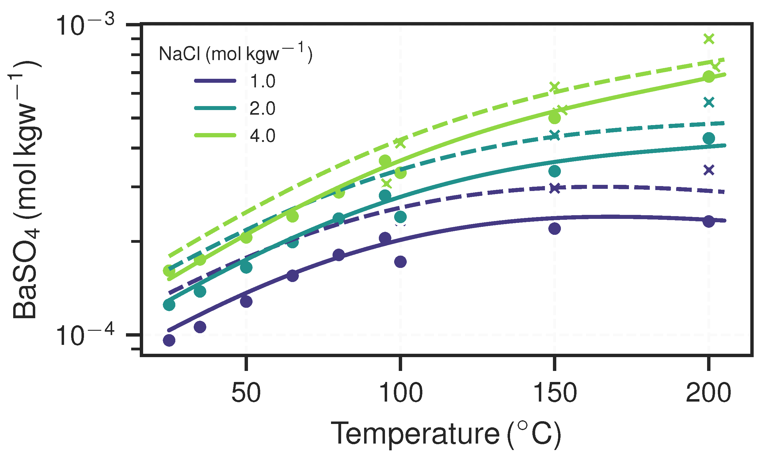
2.1.2. Equilibrium Models and Barite Scaling Potential

The well established software phreeqc (U.S. Geological Survey) [42], version 3.6, was used to do all geochemical batch calculations. The pre-shipped database pitzer.dat was applied, which provides thermodynamic data for calculating temperature- and pressure-dependent solubility products of many common minerals, as well as coefficients for the Pitzer ion-interaction activity model [43]. It has been shown that using this database yields good results for predicting barite solubility at high ionic strengths up to 6 M [18].
The equilibrium reaction of barite in an aqueous solution is defined as:
BaSO 4 ( solid ) Ba ( aq ) 2 + + SO 4 ( aq ) 2
Based on the law of mass action, the saturation state of barite in a solution is calculated with
SR barite = Ba 2 + · SO 4 2 K sp , barite · γ Ba 2 + · γ S O 4 2
where SR barite is the saturation ratio, K sp , barite is the temperature- and pressure-dependent solubility constant and γ i is the activity coefficient of the respective species. A solution is undersaturated if SR barite < 1 and supersaturated if SR barite > 1 . The relationship of solubility with regards to temperature, pressure and NaCl -equivalent ionic strength is shown in Figure 2.
Furthermore, the initial ratio of the aqueous SO 4 2 and Ba 2 + concentrations constrains the total precipitation amount, which follows from Equations (1) and (2). To illustrate this, two unitless example cases are considered: (A) a 1 = 1 and a 2 = 1 ; and (B) b 1 = 0.5 and b 2 = 2 . Both have the same initial product: ζ = a 1 · a 2 = b 1 · b 2 = 1 , but their ratios differ. If, for both cases, the two reactants are reduced uniformly due to precipitation by 0.1, the resulting products are ζ A = 0.9 · 0.9 = 0.81 and ζ B = 0.4 · 1.9 = 0.76 . The product for the case B reduces more strongly and equilibrium is reached earlier. Therefore, the stronger the initial ratio deviates from unity, the less precipitation can be expected at thermodynamic equilibrium. The resulting ion ratios of the cases are shown in Table 1.
The target Mesozoic sandstones predominantly consist of quartz. Accessory barite content is reported to exist in the host rock in both regions [44,45], with concentrations ranging from 100 to 300 ppm (maximum 1000 ppm ). It appears paragenetically next to minerals, such as anhydrite, celestite and calcite, or in fracture fillings [44]. Aqueous Ba -concentrations are only provided for the reservoir fluids of NG and LND. Based on these compositions, the fluids appear to be close to equilibrium with respect to barite at reservoir conditions. Thus, the commonly applied assumptions is used that the fluids are in equilibrium with the mineral assemblage of the formation rock [46]. As the starting point for all consecutive equilibrium and reactive transport calculations, the concentrations reported in the literature were adjusted to achieve equilibrium with all mentioned minerals (Table 1). The Cl -content was adjusted to achieve charge balance.
The maximum barite scaling amount was derived from equilibrium modelling by changing the initial P and T state with respect to the production–injection cycle (Figure 1). Re-injection temperatures usually lie in the range 45–65 C . The system pressure usually is in the order of 1 MPa [47,48]. P increases again at the injection well, which is in the order of the reservoir’s down-hole pressure. The concentration difference between the initial and altered state represents the maximum amount of barite that can precipitate from the thermodynamic point of view.

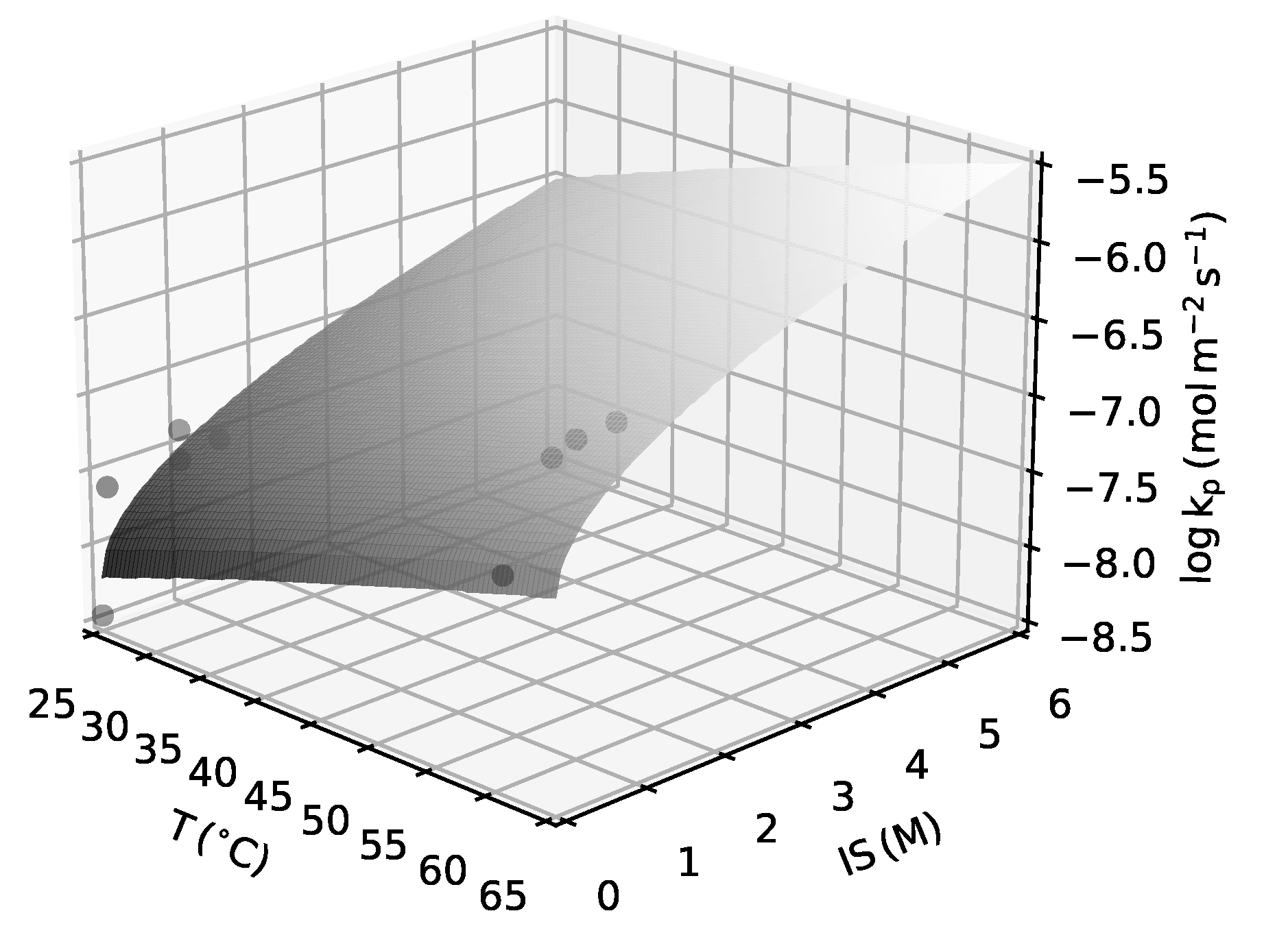
2.1.3. Crystal Growth Kinetics

Crystal growth kinetics were considered in order to yield information on time and therefore location of scale formation. Pristine barite content in the rock matrix constitutes growth sites. Nucleation from solution can lead to an increase in the amount of active growth sites over time. This process was disregarded here, however, because the respective supersaturation ratios are assumed to be too low in the investigated cases for it to be growth determining. The reactive surface area of the available barite S barite ( m 2 m 3 ) determines the magnitude of the reaction rate, which was approximated using
S barite = ϕ barite · S · SF
where ϕ barite ( m 3 m 3 ) is the initial volume fraction of barite in the rock, S ( m 2 m 3 ) is the specific inner surface area of the rock and SF is a dimensionless scaling factor for converting the specific into the effective reactive surface area. S was assumed to be 3 · 10 4 m 2 m 3 for the considered sandstones [2,49]. Barite was found to exist in aggregations or fracture veins [44], hence it was assumed that fluid accessibility is reduced. SF was therefore set to 0.05 in order to account for the reduced volume fraction that is accessible to the pore network [50]. From measured weight fractions of the mineral assemblage, the volume fraction of barite is
ϕ barite = ( 1 ϕ ) w barite ρ barite w barite ρ barite + 1 w barite ρ quartz
where w barite ( kg kg 1 ) is the weight fraction of barite in the rock and ρ i ( kg m 3 ) is the respective density of barite ( = 4480 kg m 3 ) and quartz ( = 2650 kg m 3 ). Note that, for the sake of simplicity, only quartz and barite were assumed to be in the rock for these calculation. The weight fraction of barite in the Bunter sandstones is reported to be in the range 0.01 0.10 wt% [44] in the NGB or in traces [45] in the URG, hence 0.10 wt % was used to have a conservative estimate.
A general formulation of the reaction mechanism was applied [22]:
R = k p ( 1 SR )
where R ( mol m 2 s 1 ) is the surface area normalised precipitation rate and k p is the temperature and ionic strength dependent rate constant. It has been shown that it is independent from pH in the range 3–9 [30]. k p was fitted from experimental data [32] using a first-order linear regression by minimising the averaged residuals (see Appendix A.1). The resulting empirical expression is:
log 10 k p = 2532 ( T + 273 ) + 0.694 IS + 0.29
where T ( C ) is the temperature and IS ( M ) is the ionic strength. An extrapolation outside of these ranges can be seen in Figure 3.

2.2. Flow

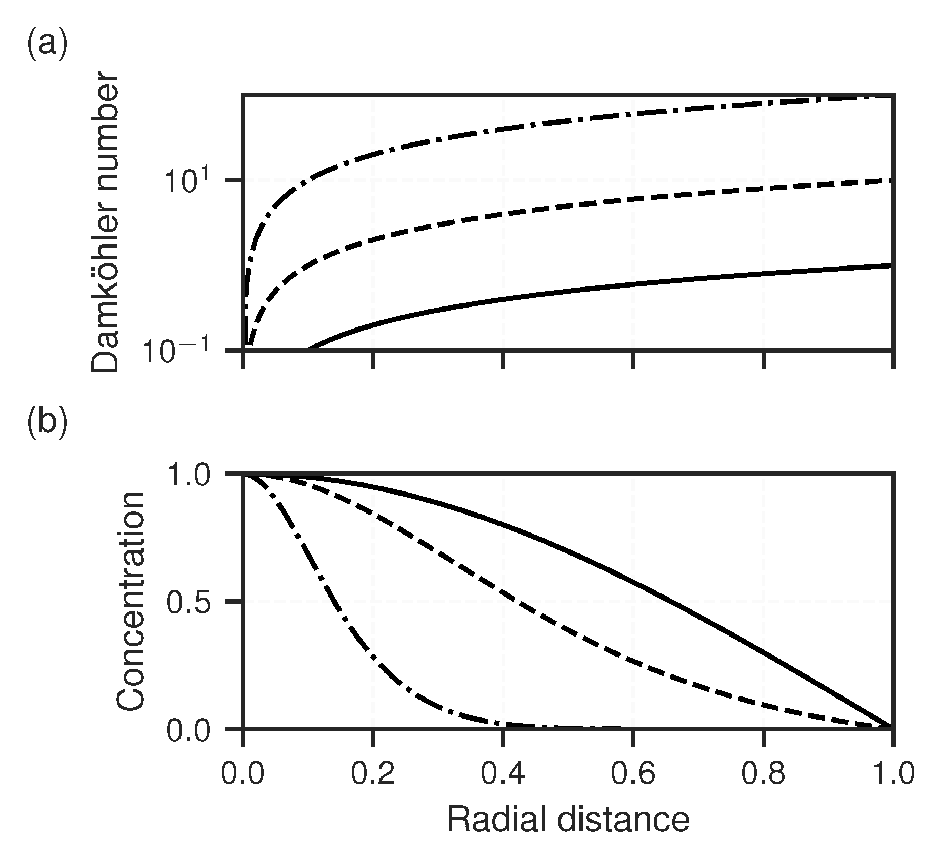
2.2.1. Reservoir Hydraulics

The injectivity index J ( m 3 s 1 Pa 1 ) quantifies an injection well’s efficiency in terms of flow rate Q ( m 3 s 1 ) and corresponding pressure build-up d P ( Pa ) . The applied pressure difference follows from the planned flow rate and the transmissivity of the target reservoir. It can be approximated with the Dupuit–Thiem well equation, if Darcy flow is assumed [51]:
Q = 2 π T s ln r e r w
where T ( m 2 s 1 ) is the transmissivity, s ( m ) is the water column corresponding to the pressure build-up, r e ( m ) is the reach of the pressure difference and r w ( m ) is the well radius. Transmissivity and reach are both determined by permeability K ( m 2 ) , hence solving this equation with regards to s must be done iteratively using an adequate relationship for r e and K. However, in the following, it suffices to consider only the relative injectivity loss resulting from pore clogging. It can be shown that it approximately equals permeability loss if the reach is large compared to the well bore radius ( r e r w ).
Franz et al. [52] reported that circulation rates need to be around 100 m 3 h 1 in order to achieve the necessary thermal output for a profitable and long-term operation. Higher reservoir temperatures compensate lower flow rates and vice versa. Further, J should be at least 50 m 3 h 1 MPa 1 in order to achieve these circulation rates with realistic pressure differences. The minimum hydraulic parameters for a porous hydrothermal reservoir are given it Table 2. K, M and ϕ constitute mean reservoir properties and were accepted to be the starting point for all cases in order to compare them with regards to barite scale formation. All reservoirs were thus simplified in the models to isotropic and homogeneous porous aquifers.

2.2.2. Reactive Transport Modelling
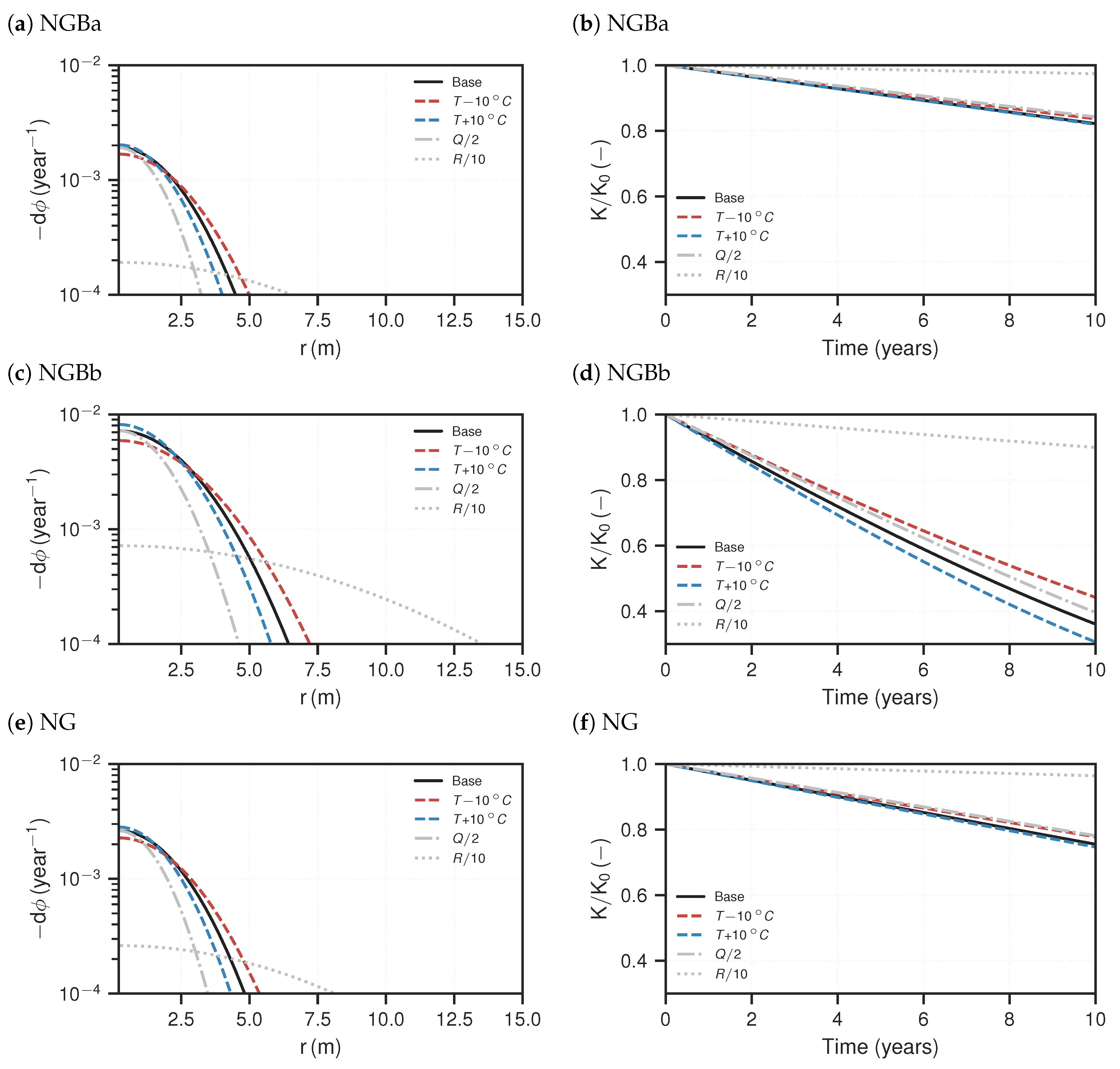
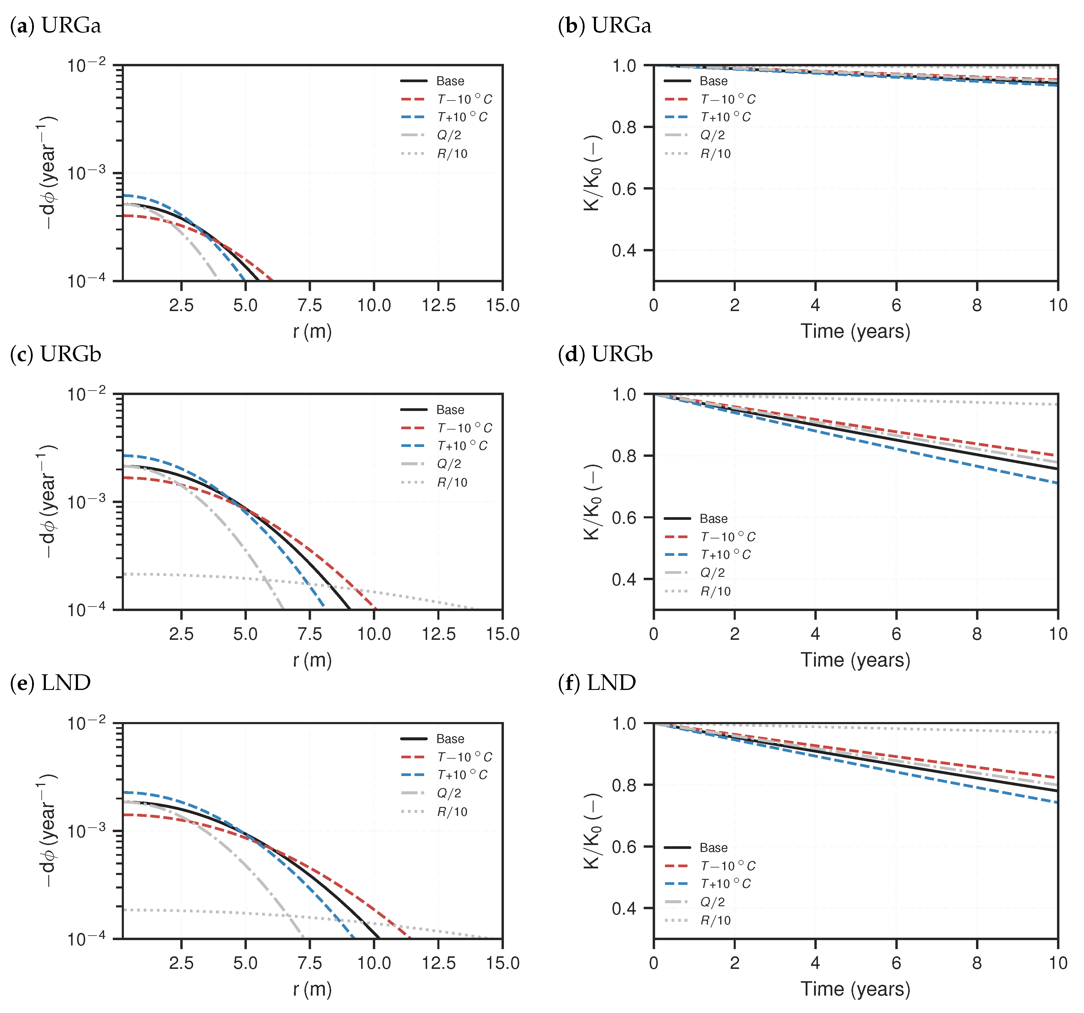
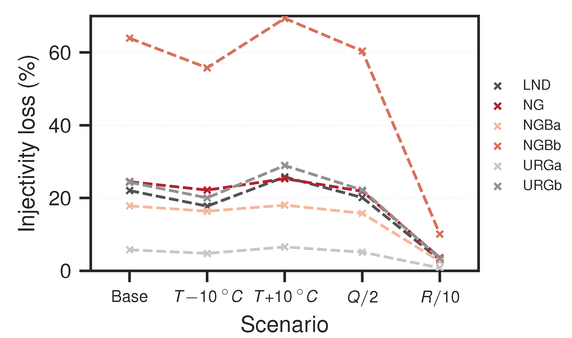
Flow from an injection well into a porous aquifer can be described by radially diverging flow [53,54]. If the regional hydraulic gradient is neglected and assuming homogeneous and isotropic flow properties of the aquifer, the injection well exhibits radial symmetry. Further, for fully penetrating injection wells, flow can be assumed to be planar and horizontal. Thus, a one-dimensional reactive transport model was set up to model the injection of supersaturated fluids into the aquifer. The governing equations are given in Appendix A.2.
To take barite precipitation kinetics into account, the advection–reaction equation (Equation (A5)) is modified to:
c i t = V r c i r R S barite m water .
where c i ( M ) is the solute concentration of a respective solute species i, t ( s ) is time, V ( m 2 s 1 ) is a proxy for flow = Q / 2 π M ϕ , r ( m ) is the radial distance from the well-centre, R ( mol s 1 m 2 ) is the barite precipitation rate (Equation (5)) and m water ( kg m 3 ) is the solvent amount. Equation (8) is similar to Equation (A7), which was solved numerically and validated with an analytical solution (Appendix A.2). However, because the kinetic rate depends on changing activity coefficients, there is no straightforward analytical solution for this. Therefore, it was split and the resulting advective and reactive operators were solved separately by applying the sequential non-iterative approach. The upwind differences in space numerical method was used to solve the advection term V c i / r r . The reaction term ( R S barite / m water ) was solved with phreeqc’s batch kinetic solver, which uses an implicit Runge–Kutta algorithm [42]. A regular grid with 300 nodes and a constant time step was used, which fulfilled the Courant–Friedrich–Lewy stability criteria of the upwind scheme. Temperature and pressure were set to constant injection conditions. Solute concentrations ( Ba 2 + and SO 4 2 ) at the inlet boundary were taken from equilibrated, initial reservoir data. All other species were used as constant background concentration. V and S barite were kept constant during a simulation, as feedback from reaction on flow or reactive surface area were not taken into account. The solute concentration profiles therefore reached steady-state at one point.
The shape of such steady-state concentration profiles are determined by the relationship of advection to reaction. If advection is increased, the profiles will be flattened and vice versa. A way to describe this relationship is to use the dimensionless Damköhler number Da [55]:
Da ( r ) = r r c V R ϕ c i , eq
where r c ( m ) is a characteristic length set arbitrarily to 15 m . It follows that Da is a linearly increasing function along the flow path r, since all other parameters were assumed to be constant. The steeper is this function, the shorter is the equilibrium length scale and precipitation can be expected to happen closer to the point of origin. This is illustrated in Figure 4 for various Da -slope values. The slope of Da ( r ) can be calculated simply with:
m Da = dDa d r = Da ( r ) r
or written out:
m Da = r c V R ϕ c i , eq = 2 π M r c Q R c i , eq
Barite precipitation leads to porosity decrease, which can be expressed by volume fraction:
d ϕ barite d t = V m , barite R
where V m , barite is the molar volume of barite. From this expression, the altered porosity was obtained for each domain node. Note that only quartz and barite were taken into account. To approximate the change in permeability, the widely used Kozeny–Carman relationship was applied [56,57]:
K j K 0 = ϕ j 3 ( 1 ϕ 0 ) 2 ϕ 0 3 ( 1 ϕ j ) 2
where ϕ 0 and ϕ j are the initial porosity and porosity at time step j, respectively. The effective permeability follows from a series of blocks; it was calculated using the harmonic mean of the individual blocks’ permeability [58]. Due to the radial diverging flow field, the logarithmic harmonic mean must be used:
K = ln r n r w j = 1 n ln r j r j 1 K j
where r j is the radial distance of a node j from the center of the injection well and r w is the well radius. r n was chosen so as to capture the saturation length scale.
The order of steps used for assessing the temporal permeability loss is as follows:
  • Calculate reactive surface area (Equation (3)).
  • Calculate rate constant (Equation (6)).
  • Calculate flow constant V.
  • Evaluate Damköhler number along the r-axis (Equation (9)) and the corresponding slope (Equation (11)).
  • Solve ARE (Equation (8)) with numerical simulations until solutes reach steady-state.
  • Extrapolate porosity change at steady-state for each node over ten years.
  • Evaluate permeability loss using both the porosity–permeability relationship (Equation (13)) and the effective permeability expression for the radial diverging flow field (Equation (14)).
Each geothermal sample case was evaluated this way, representing the respective base scenario by using values described in the previous sections (Table 1 and Table 2). To illustrate the effects of various parameters on the simulation results, additional scenarios were examined as in a one-at-a-time sensitivity analysis (Table 3).

3. Results

3.1. Equilibrium Models

The scaling potential results from equilibrium calculations are shown in Figure 5. The whole range from the respective reservoir temperature down to 25 C illustrates the effect of temperature reduction, expressed as d T = T res T i . Furthermore, the influence of pressure reduction d P from reservoir to surface condition is shown.
Figure 5a presents the respective barite saturation associated to d T and d P . The curves show an exponentially increasing trend for all cases with increasing d T . The URG cases (grey tones) generally exhibit higher saturation ratios than the NGB cases (red tones) at equal depths. The considered pressure reduction additionally increases the saturation, however not as strongly as the accompanying temperature reduction. With regards to the flow path in geothermal installations, saturation increases during the passageway through the production well and the heat exchanger due to temperature and pressure reduction, respectively. Supersaturation reaches its highest magnitude up to the point where the fluid is pressurised again and re-injected through the injection well. Assuming a temperature and pressure reduction down to 55 C and 1 MPa , respectively, SR values for the various cases lie between 3.2 and 7.1 . If these values overstep the supersaturation threshold, nucleation can be expected in the surface installation. SR values representative for the injection location are between 2.7 and 5.3 , which are lower again due to the increased fluid pressure.
Figure 5b presents the associated total amount of barite that can precipitate from a cubic metre of produced formation fluid, which has been subjected to change in temperature and pressure. The cases representing greater depths (NGBb, URGb and LND) have a higher scaling potential than the shallower cases (NGBa, URGa and NG). With regards to fluid injection, values lie between 74 and 88 mmol m 3 and 12 and 23 mmol m 3 for the deeper and shallower cases, respectively. The results at injection conditions are also shown in Table 4. Lower injection temperatures result in more scaling potential, although the curve flattens off, meaning that it does not grow linearly. This further indicates that the potential scaling amount is not linearly correlated to the previously reported exponentially increasing saturation ratios. Generally, the higher the fluid’s ionic strength, the more scaling can be expected. The same applies to the degree of temperature and pressure reduction, although the drop from reservoir to system pressure has a generally smaller effect on precipitation than temperature. The NGB cases tend to exhibit higher values, although their d T values to reach injection temperature are lower. For instance, temperature reduction for the NGBb case is close to half compared to the URGb case, however scaling potential is almost 20 % higher for the NGBb case.
The initial ion ratios of aqueous SO 4 2 and Ba 2 + are shown in Table 1. SO 4 2 concentrations are generally higher, between 30 and 300 times the concentration of Ba 2 + . The ratios of the deeper cases are about one order closer to unity than the shallower cases. Cases with ion ratios closer to unity are reflected in steeper curve slopes in Figure 5b.

3.2. Reactive Transport Models

The Damköhler number increases linearly for the considered flow model, originating from zero along the r-axis. The associated slopes m Da (Equation (10)) for all scenarios are shown in Table 4. The higher is m Da , the faster is the advection time decreases along the r-axis compared to the reaction rate, and thus the more precipitation will occur more concentrated close to the injection well. All URG cases have comparably low slope values, whereas the NGBa and NG cases have the highest values. Reducing the flow rate increases while reducing the reaction rate reduces m Da proportionally. In accordance with the kinetic rate expression (Equation (6)), increasing temperature increases m Da .
In the following, the reactive transport simulation results are presented. In Figure 6 and Figure 7, the NGB and URG cases are shown, respectively. On the left-hand side, the temporal porosity changes at steady-state are plotted against the r-axis. Porosity changes result from increase of barite volume fraction. Note that the porosity change plots are cut off at 10 4 per year, as lower values are assumed to be negligible with regards to their impact on permeability during the life time of a geothermal installation. This corresponds to a porosity loss of 0.1 % over the course of ten years. All curves show flipped parabola shapes in the semi-log plot, with the porosity change maximum close to the origin, i.e., the outflow of the injection well. The NGBb case generally exhibits the highest porosity changes with a maximum of 0.7 % porosity loss per year. The URGa case has the least loss of more than one order of magnitude less than that of NGBb. It can be seen that the URG cases have flatter curves and broader widths of significant precipitation along the axis. Precipitation is concentrated closer to the well for the NGB cases. They have ranges of about 4.5 6.5 m , compared to 5.5 10.5 m for the URG cases.
Changing the injection temperature within in the considered ranges of the sensitivity analysis only has a small effect compared to the base case. A temperature increase accelerates precipitation and vice versa. As such, lower injection temperature increases the reach and also lowers the maximum porosity decline close to the well. Smaller flow rates generally result in less precipitation in total, which can be anticipated by the total area under the curves; compared to the base case, the maximum porosity changes at the inlet still has the same order of magnitude, however the reach is reduced by about 30 % . Lower reaction rates (R) flatten the curves quite significantly, meaning precipitation is more distributed along the flow path. If the magnitude of R is one order lower compared to the base case, the porosity change peak is also one order of magnitude lower and the reach is increased by about 50 % .
The associated temporal permeability ratios ( K / K 0 ) over the course of ten years are shown on the right-hand side of Figure 6 and Figure 7. Notably, all curves illustrate a linear decline of permeability over time. The related injectivity losses per year ( 1 K / K 0 ) are shown in Table 4. In the base case, the NGBb case exhibits the strongest permeability decline by over 6 % per year. It slightly deviates from a linear curve towards the end of the considered time. The URGa case shows the lowest permeability decline of just below 0.6 % per year; the others have between 1.8 % and 2.4 % loss per year. With regards to the sensitivity analysis scenarios, change in reactivity has the strongest impact on the permeability decline. If the reaction rate is reduced by one order of magnitude compared to the base case, the resulting permeability loss after 10 years is also reduced by almost one order of magnitude. For the shallower cases (NGBa, URGa and NG), the other sensitivity analysis scenarios with regards to temperature and flow rate show only negligible deviations from the base case. For the deeper cases (NGBb, URGb and LND), increasing temperature (lower d T ) accelerates permeability loss and decreasing temperature (higher d T ) slows the decline down. Decreasing the flow rate reduces the permeability loss. However, this effect is small, about 10 % deviation from the base case.
The final effective permeability changes after ten years for all investigated cases and scenarios are summarised in Figure 8. It can be seen that the reservoirs of greater depth generally are affected more strongly by permeability losses. The NGB cases are generally affected more strongly than the URG cases; NGBb has by far the highest permeability loss ( 64 % ). Further, NG is similarly affected than URGb and LND, although it is not as deep; all exhibit a loss of approximately 24 % . URGa has the least loss of just below 6 % . Again, for all shallower cases (NG, NGBa and URGa), varying injection temperature or flow rate only has a little to no effect compared to the base case. There is a noticeable effect, however, with regards to injection temperature variation for the deep cases. As such, decreasing temperature reduces the permeability loss, whereas increasing temperature results in more loss. If reactivity is reduced compared to the base case, permeability loss is significantly less. Especially for the NGBb case, loss after ten years drops down from 64 % to only 10 % in this scenario. The loss of the URGa case goes down to virtually zero in this scenario.

4. Discussion

Total barite scaling potential is determined by fluid composition, temperature reduction, pressure reduction and ion ratio of Ba 2 + and SO 4 2 . For the presented geothermal cases in the NGB and the URG, formation fluid temperature and salinity increase with greater reservoir depth. The deeper cases also showed ion ratios closer to unity. These factors all increase the precipitation potential and thus increase the scaling risk for deeper reservoirs. Furthermore, for cases at similar depths, fluid salinity is higher in the NGB and temperature is higher in the URG, but total scaling potential is in the same order of magnitude. As the corresponding saturation ratios were significantly higher for the URG cases, this illustrates that these values are not linearly correlated. Saturation ratios can only be taken as an indication of whether precipitation can be expected or not. Scaling amounts need to be investigated in detail for a specific location, taking the mentioned factors into consideration.
An irreversible injectivity decline of about 35 % after 16 years of injection has been reported at the geothermal site Neustadt-Glewe [13]. The authors attributed this mainly to formation of sparingly soluble scales in the reservoir, such as barite, celestite and various sulfides [9,13]. This order of magnitude is in fact in accordance with calculated injectivity losses, even though only barite scaling was taken into consideration in the present study. In this regard, some conservative assumptions were made, to the effect that the upper range of risk associated to barite scaling was assessed. For instance, it was assumed that barite growth does not happen until the re-injected fluid comes into contact with active growth sites (solid barite) in the formation rock. Precipitation rate and injectivity loss are further increased. Formation of additional active growth sites can occur through nucleation, increasing the precipitation and injectivity loss rate further. Whether this effect is significant depends on site characteristics such as mineralogy of the in-situ rock. This process was disregarded in the models, hence the real precipitation rate will be underestimated to some degree. For the considered cases, nucleation was not considered to be a growth determining step, as the highest saturation ratios were presumed to be too low for this [59,60]. Nuclei formation can be promoted, however, by longer shut-in periods [10,11,36]. As a consequence, scale formation sets in prior to the fluid reaching the formation rock, thus not affecting the injectivity as strongly, but perhaps with other unwanted impediments [10]. Furthermore, re-injected fluids heat-up again gradually in the reservoir, depending on flow rate and heat transfer, which has not been taken into consideration. This increases barite solubility again and thus reduces scaling risk, more so if flow rate is reduced. In light of the simulated scaling reach of below 10 m , however, this effect appears to be negligible. On the other hand, injection pressure must be increased to maintain injection rates if permeability decreases. This could pose problems, as this increases the chance for loose particles to redistribute and clog pores. This process, however, is hard to quantify and also was not considered.
Supersaturation and kinetic rate both depend on the fluid’s salinity and temperature. An increase in salinity therefore increases the precipitation rate two-fold. The relationship with regards to temperature is different: supersaturation increases further with temperature reduction (increased d T ), whereas the rate constant is proportional to the absolute temperature. For quartz scaling in high-enthalpy systems, something similar was shown by Pandey et al. [61]. Reducing temperature results in a counter effect of higher supersaturation, but lower kinetic rate constant. Temperature variations as part of the sensitivity analysis had no significant impact on calculated injectivity loss, at least in the considered ± 10 C range. This explains why the NGB cases are generally affected more strongly.
Scaling potential needs to be put into perspective with regards to distribution along the flow path in order to assess implications for system longevity. Due to the radial diverging flow, large spatial distribution of scale formation means less effective permeability loss. This is promoted by slower reaction rates and higher flow velocities. The URG cases generally showed widespread distribution along the flow path, i.e., flatter precipitation curves, attributable to lower reaction rates. An important point is that equal hydraulic properties were assumed for all cases, in order to be able to compare them with regards to fluid chemistry and precipitation kinetics. While the model assumptions of radial diverging and planar flow are reasonable for homogeneous and isotropic porous aquifers with fully penetrating injection wells, they are simplifying for partially penetrating wells and especially fractured aquifers. The former have spherical flow components, thus this model treatment overestimates flow velocities and underestimates the permeability loss in the near-vicinity of the injection well for these cases. Projects in the URG rely on multi-horizontal approaches in order to minimise exploration risk [39]. Therefore, there are sections with slow flow through the porous matrix, but also sections with increased permeability due to fractures. Fracture permeability is characterised by preferential flow with increased flow velocities and also decreased water–rock contact, i.e., less effective reactive surface area. Both factors hypothetically increase the scaling distribution in the formation rock, reducing the scaling risk for the URG even further compared to the NGB.
Scaling distribution patterns in the subsurface can be described by fluid flux, total scaling potential and Damköhler number. The latter relates the respective magnitudes of advection and precipitation kinetics. Assuming that rock reactivity is homogeneous on a large scale, the Damköhler number increases linearly along the r-axis due to the radially diverging flow. The steeper is the slope ( m Da ), the closer isthe scaling distribution to the injection well. Further, the volumetric scaling potential ( n barite ) as well as fluid flux (Q) are also necessary to determine scaling in the subsurface with regards to injectivity decline, as these quantify the total amount that can precipitate from solution. In essence, these three factors provide insights into distribution and intensity of scaling in the subsurface. If they are simply lumped together, the following scaling score is derived:
X score = m Da · n barite · Q
The resulting scores for the respective cases and scenarios are provided in Table 4. They qualitatively suggest which cases’ injectivity will be affected more than others and therefore generate a ranking fit. Although this score only yields an approximation, it can nevertheless be used as a quick comparative value, without having to run elaborate reactive transport simulations. Furthermore, this scaling score is correlated with the previously calculated injectivity losses. For instance, the NGBb case has the largest values, while URGa has the lowest, which corresponds closely to the simulation results. If plotted against each other, a clear linear correlation can be seen (Figure 9). This is a valuable insight, since the calculated injectivity losses result from multiple non-linear considerations: (I) steady-state reactive transport simulations; (II) porosity–permeability relationship; and (III) effective permeability approximation. By calibrating the score with the reactive transport simulation results, the obtained linear correlation represents a lightweight score for approximating the temporal injectivity loss associated to barite scaling:
Loss ( % year 1 ) = 2.89 · 10 5 · X score ( mol m 1 year 1 )
It is easily applicable to new geothermal installations and may be calibrated further if additional data becomes available in this regard. The overall presented approach specifically treats barite as the sole scale formation agent. It can be adapted to make respective predictions for similar formation reactions of minerals exhibiting prograde solubility, for example silica or other sulfates. Though it is explicitly pointed out that the respective reaction mechanism needs detailed consideration.

5. Conclusions

Two model concepts were presented to approximate barite scaling formation in geothermal systems of the North German Basin and Upper Rhine Regions regions: an equilibrium model approach and a transport model coupled with precipitation kinetics. It was shown that temperature and pressure reduction during the production–injection cycle results in supersaturated conditions for barite in all cases, which is accountable for scaling. Equilibrium models were used to calculate the total potential scaling amount, which gives a first indication on the related risk for a long-term operation. This scaling potential increases proportionally to the imposed degree of temperature and pressure reduction dependent on the respective geothermal system management, as well as to formation fluid salinity. These parameters are generally correlated with reservoir depth. Fluids encountered at similar depths are hotter in the URG, while they are more saline in the NGB. The scaling potential is similarly high for both regions, while deeper reservoirs tend to be affected more strongly.
A comprehensive assessment of scaling risk needs to include the respective scaling location and distribution along the flow path in order to quantify the accompanied injectivity decline. From reactive transport simulations, information on both the scaling distribution in the subsurface and the related injectivity loss was obtained. Precipitation kinetics are taken into account, which also depend on temperature and salinity, similarly to the total scaling potential. Injection temperatures are usually in the same order for different geothermal installations, thus the corresponding temperature reduction ( d T ) varies. The barite precipitation rate is higher for the NGB cases due to their higher fluid salinities. Thus, scaling will preferentially happen closer to the injection well and damage reservoir permeability more severely. Therefore, the NGB cases are generally at higher risk with regards to injectivity losses, while the shallow URG case showed almost no losses. A sensitivity analysis showed that varying temperature within a 10 C margin, as well as significantly reducing the flow rate had negligible effects on injectivity loss. The kinetic rate, on the other hand, exhibited a strong sensitivity.
A scaling score was developed, which takes the total scaling potential, the Damköhler number and the flow rate into account. It correlates strongly with the results of the reactive transport simulations and may be calibrated with further data. It is easily applicable in order to get an indication on the accompanied scaling risk for a specific geothermal location, without having to run elaborate reactive transport simulations. The presented approach can be adapted to make scale formation and injectivity loss predictions for mineral formation reactions similar to that of barite.

Author Contributions

Conceptualisation, M.T. and M.K.; Formal analysis, M.T.; Funding acquisition, M.K.; Investigation, M.T.; Methodology, M.T., M.D.L. and M.K.; Project administration, M.K.; Resources, M.W.; Software, M.T.; Supervision, M.K.; Writing—original draft, M.T.; and Writing—review and editing, M.D.L., M.W. and M.K. All authors have read and agreed to the published version of the manuscript.

Funding

This research has been supported by the Federal Ministry for Economics and Energy of Germany BMWi (grant no. 0324244C, project ReSalt).

Conflicts of Interest

The authors declare that they have no conflict of interest.

Abbreviations

The following abbreviations are used in this manuscript:
AbbreviationDescriptionUnit
c i Concentration M
c i , eq Concentration in equilibrium M
Da Damköhler number
γ i Activity coefficient
iAqueous species or solid
IS Ionic strength M
jGrid node
JInjectivity m 3 s 1 Pa 1
KRock permeability m 2
K 0 Initial rock permeability m 2
k p Precipitation rate constant mol m 2 s 1
K sp Solubility constant mol 2 kg 2
LND Landau
MAquifer thickness m
m Da Da slope along the r-axis m 1
m water Water mass kg
n i Precipitation potential mol
NG Neustadt-Glewe
NGB North German Basin
PPressure Pa
ϕ Porosity
ϕ 0 Initial porosity
ϕ i Volume fraction
QFlow rate m 3 s 1
rRadial distance from well-centre m
RBarite precipitation rate (surface area normalised) mol m 2 s 1
r c Characteristic length m
r e Reach of pressure difference m
r w Well radius m
ρ i Density of solid kg m 3
ρ s Density of fluid kg m 3
sWater column m
SSpecific inner rock surface m 2 m 3
S i Reactive surface area m 2
SF Scaling factor for reactive surface area
SR i Supersaturation ratio
TTemperature C
T inj Injection temperature C
TDS Total dissolved solids kg
URG Upper Rhine Graben
VFlow constant (=Q / 2 π M ϕ ) m 2 s 1
w i Weight fraction kg kg 1
X score Scaling score mol m 1 year 1

Appendix A. Reactive Transport Simulations

Appendix A.1. Kinetic Rate Constant

The kinetic rate constant k p for bulk precipitation of barite was derived from unseeded batch experiments at low supersaturation SR < 8 [32]. k p is temperature and ionic strength dependent. It was fitted with a first-order linear regression by minimising the averaged residuals:
log 10 k p = 2532 ( T + 273 ) + 0.694 IS + 0.29
where T ( C ) is the temperature and IS ( M ) is the ionic strength. The data are given in Table A1. The underlying experimental data were conducted in the ranges 25–60 C and 0– 1.5 M .
Table A1. Rate constants for bulk precipitation of barite at varying conditions used for the linear regression. The parameters T and IS are the input factors. Comparing experimental and model rates yields R adj 2 = 0.88 .
T IS log 10 k p , exp a log 10 k p , model
C mol kgw 1 NaCl mol m 2 s 1 mol m 2 s 1
25 0.0 8.46 8.21
25 0.1 7.62 7.99
25 1.0 7.60 7.51
25 1.5 7.55 7.36
60 0.1 7.22 7.09
60 0.7 6.60 6.73
60 1.0 6.54 6.62
60 1.5 6.52 6.46
25 1.0 7.40 7.51
a Experimental data on bulk precipitation [32].

Appendix A.2. Governing Equations and Analytical Solution

In the following, the applied reactive transport equations and their solution approaches are derived. The general one-dimensional advection–diffusion–reaction equation can be written in Cartesian coordinates [54]:
c i t = · ( D c i ) · ( v c i ) + R i
In the vicinity of the injection well, the advective component of flow dominates, thus the equation reduces to
c i t = · ( v c i ) + R i .
v x is dependent on x (Figure A1) for radially diverging flow resulting from an injection well. Further, assuming homogeneous and isotropic conditions, we can transform Equation (A3) into cylindrical coordinates by using the velocity tensor
v = v r = Q 2 π r M ϕ = V r v φ = 0 v z = 0
in
c i t = V r c i r + R i .
For the steady-state case, this further reduces to
V r c i r + R i = 0 .
In the above equations, the subscript i denotes a respective solute species, c ( N L 3 ) is the solute concentration in the radial flow field, r ( L ) is the radial distance from the center of the injection well, x ( L ) is the distance from the injection well in Cartesian coordinates, t ( T ) is time, D ( L 2 T 1 ) is the hydrodynamic dispersion, Q ( L 3 T 1 ) is the injection flow rate, M ( L ) is the thickness of the aquifer, ϕ is porosity, R ( N L 3 T 1 ) is a solute source ( > 0 ) or sink ( < 0 ) term and V ( L 2 T 1 ) is a flow constant.
An analytical solution is derived to validate the applied numerical method against. The sink term R i in Equation (A6) is set to a simple zeroth order reaction rate, resulting in
V r c i r μ i ( c i c i , eq ) = 0
where c i , eq is the equilibrium concentration and μ i is the reaction rate of a reacting solute species i. The general form of the solution of Equation (A7) then reads:
c i ( r , t ) = c i , eq + exp μ i r 2 + 2 F ( t ) 2 V
We consider the IBVP with initial concentration c i , eq and injection of a constant concentration c i = c i , 0 > c i , eq at the origin of the coordinate systems r = 0 :
c i ( r , 0 ) = c i , eq c i ( 0 , t ) = c i , 0
By plugging Equation (A9) into Equation (A8), we get the following definition for F:
F ( t ) = V ln c i , 0 c i , eq
Finally, by inserting Equation (A10) into Equation (A8), we get to write the full analytical steady-state solution:
c i ( r , t ) = c i , eq + ( c i , 0 c i , eq ) exp μ i r 2 2 V , for r > 0 , t > 0
The first-order upwind differences in space method can be used to solve Equation (A7) numerically:
c i , j n + 1 = c i , j n V r j d t d r ( c i , j n c i , j 1 n ) d t μ i ( c i , j n c i , eq )
where superscript n represents the time step; subscripts i and j represent a solute species and the domain node, respectively; d t is the time step length; and d r is the grid length. This scheme is stable for d t min d r r j / V . Up to j iterations are necessary to reach steady-state. Equations (A11) and (A12) are compared in an example steady-state case, which can be seen in Figure A1.
Figure A1. (top) The decline of the flow velocity along the r-axis due to the diverging flow; and (bottom) the comparison of the analytical and numerical solutions for solving Equation (A7). The solid line and dots represents the analytical and numerical solution, respectively.
Water 12 03078 g0a1

References

  1. Agemar, T.; Weber, J.; Schulz, R. Deep Geothermal Energy Production in Germany. Energies 2014, 7, 4397–4416. [Google Scholar] [CrossRef]
  2. Schumacher, S.; Pierau, R.; Wirth, W. Probability of Success Studies for Geothermal Projects in Clastic Reservoirs: From Subsurface Data to Geological Risk Analysis. Geothermics 2020, 83, 101725. [Google Scholar] [CrossRef]
  3. Wolfgramm, M.; Thorwart, K.; Rauppach, K.; Brandes, J. Zusammensetzung, Herkunft Und Genese Geothermaler Tiefengrundwässer Im Norddeutschen Becken (NDB) Und Deren Relevanz Für Die Geothermische Nutzung. Z. Geol. Wiss. 2011, 339, 173–193. [Google Scholar]
  4. Pauwels, H.; Fouillac, C.; Fouillac, A.M. Chemistry and Isotopes of Deep Geothermal Saline Fluids in the Upper Rhine Graben: Origin of Compounds and Water-Rock Interactions. Geochim. Cosmochim. Acta 1993, 57, 2737–2749. [Google Scholar] [CrossRef]
  5. Stober, I.; Wolfgramm, M.; Birner, J. Hydrochemie Der Tiefenwässer in Deutschland. Z. Geol. Wiss. 2013, 42, 339–380. [Google Scholar]
  6. Naumann, D. Salinare Tiefenwässer in Norddeutschland: Gas- und Isotopengeochemische Untersuchungen zur Herkunft und Geothermische Nutzung; Scientific Technical Report STR00/21; Deutsches GeoForschungsZentrum Potsdam: Potsdam, Germany, 2000. [Google Scholar]
  7. Sanjuan, B.; Millot, R.; Innocent, C.; Dezayes, C.; Scheiber, J.; Brach, M. Major Geochemical Characteristics of Geothermal Brines from the Upper Rhine Graben Granitic Basement with Constraints on Temperature and Circulation. Chem. Geol. 2016, 428, 27–47. [Google Scholar] [CrossRef]
  8. Wolfgramm, M.; Seibt, A. Zusammensetzung von Tiefenwässern in Deutschland Und Ihre Relevanz Für Geothermische Anlagenteile. In Proceedings of the Der Geothermiekongress 2011, Rheinstetten, Germany, 11–13 November 2008. [Google Scholar]
  9. Wolfgramm, M.; Rauppach, K.; Thorwart, K. Mineralneubildung Und Partikeltransport Im Thermalwasserkreislauf Geothermischer Anlagen Deutschlands. Z. Geol. Wiss. 2011, 39, 213–239. [Google Scholar]
  10. Regenspurg, S.; Feldbusch, E.; Byrne, J.; Deon, F.; Driba, D.L.; Henninges, J.; Kappler, A.; Naumann, R.; Reinsch, T.; Schubert, C. Mineral Precipitation during Production of Geothermal Fluid from a Permian Rotliegend Reservoir. Geothermics 2015, 54, 122–135. [Google Scholar] [CrossRef]
  11. Nitschke, F.; Scheiber, J.; Kramar, U.; Neumann, T. Formation of Alternating Layered Ba-Sr-Sulfate and Pb-Sulfide Scaling in the Geothermal Plant of Soultz-Sous-Forêts. Neues Jahrb. Mineral. J. Mineral. Geochem. 2014, 191, 145–156. [Google Scholar] [CrossRef]
  12. Seibt, P.; Kabus, F.; Wolfgramm, M.; Bartels, J.; Seibt, A. Monitoring of Hydrogeothermal Plants in Germany—An Overview. In Proceedings of the World Geothermal Congress, Bali, Indonesia, 25–30 April 2010. [Google Scholar]
  13. Birner, J.; Seibt, A.; Seibt, P.; Wolfgramm, M. Removing and Reducing Scalings—Practical Experience in the Operation of Geothermal Systems. In Proceedings of the World Geothermal Congress, Melbourne, Australia, 16–24 April 2015. [Google Scholar]
  14. Scheiber, J.; Seibt, A.; Birner, J.; Genter, A.; Moeckes, W. Application of a Scaling Inhibitor System at the Geothermal Power Plant in Soultz-Sous-Forêts: Laboratory and On-Site Studies. In Proceedings of the European Geothermal Congress, Pisa, Italy, 3–7 June 2013. [Google Scholar]
  15. Agemar, T.; Schellschmidt, R.; Schulz, R. Subsurface Temperature Distribution in Germany. Geothermics 2012, 44, 65–77. [Google Scholar] [CrossRef]
  16. Blount, C.W. Barite Solubilities and Thermodynamic Quantities up to 300 C and 1400 Bars. Am. Miner. 1977, 62, 942–957. [Google Scholar]
  17. Templeton, C.C. Solubility of Barium Sulfate in Sodium Chloride Solutions from 25 to 95 C. J. Chem. Eng. Data 1960, 5, 514–516. [Google Scholar] [CrossRef]
  18. Hörbrand, T.; Baumann, T.; Moog, H.C. Validation of Hydrogeochemical Databases for Problems in Deep Geothermal Energy. Geotherm. Energy 2018, 6. [Google Scholar] [CrossRef]
  19. Bozau, E.; Häußler, S.; Van Berk, W. Hydrogeochemical Modelling of Corrosion Effects and Barite Scaling in Deep Geothermal Wells of the North German Basin Using PHREEQC and PHAST. Geothermics 2015, 53, 540–547. [Google Scholar] [CrossRef]
  20. Haarberg, T.; Selm, I.; Granbakken, D.B.; Ostvold, T.; Read, P.; Schmidt, T. Scale Formation in Reservoir and Production Equipment During Oil Recovery: An Equilibrium Model. SPE Prod. Eng. 1992, 7, 75–84. [Google Scholar] [CrossRef]
  21. Schröder, H.; Teschner, M.; Köhler, M.; Seibt, A.; Krüger, M. Long Term Reliability of Geothermal Plants—Examples from Germany. In Proceedings of the European Geothermal Congress, Unterhaching, Germany, 30 May–1 June 2007. [Google Scholar]
  22. Lasaga, A.C. Kinetic Theory in the Earth Sciences; Princeton University Press: Oxfordshire, UK, 1998. [Google Scholar]
  23. Phillips, O.M. Flow and Reactions in Permeable Rocks; Cambridge University Press: Cambridge, UK, 1991. [Google Scholar]
  24. Beckingham, L.E. Evaluation of Macroscopic Porosity-Permeability Relationships in Heterogeneous Mineral Dissolution and Precipitation Scenarios. Water Resour. Res. 2017, 53, 10217–10230. [Google Scholar] [CrossRef] [Green Version]
  25. Gardner, G.L.; Nancollas, G.H. Crystal Growth in Aqueous Solution at Elevated Temperatures. Barium Sulfate Growth Kinetics. J. Phys. Chem. 1983, 87, 4699–4703. [Google Scholar] [CrossRef]
  26. Godinho, J.R.; Stack, A.G. Growth Kinetics and Morphology of Barite Crystals Derived from Face-Specific Growth Rates. Cryst. Growth Des. 2015, 15, 2064–2071. [Google Scholar] [CrossRef]
  27. Christy, A.G.; Putnis, A. The Kinetics of Barite Dissolution and Precipitation in Water and Sodium Chloride Brines at 44–85 C. Geochim. Cosmochim. Acta 1993, 57, 2161–2168. [Google Scholar] [CrossRef]
  28. Liu, S.T.; Nancollas, G.H.; Gasiecki, E.A. Scanning Electron Microscopic and Kinetic Studies of the Crystallization and Dissolution of Barium Sulfate Crystals. J. Cryst. Growth 1976, 33, 11–20. [Google Scholar] [CrossRef]
  29. Nancollas, G.H.; Purdie, N. Crystallization of Barium Sulphate in Aqueous Solution. Trans. Faraday Soc. 1963, 59. [Google Scholar] [CrossRef]
  30. Ruiz-Agudo, C.; Putnis, C.V.; Ruiz-Agudo, E.; Putnis, A. The Influence of pH on Barite Nucleation and Growth. Chem. Geol. 2015, 391, 7–18. [Google Scholar] [CrossRef]
  31. Risthaus, P.; Bosbach, D.; Becker, U.; Putnis, A. Barite Scale Formation and Dissolution at High Ionic Strength Studied with Atomic Force Microscopy. Colloids Surf. Physicochem. Eng. Asp. 2001, 191, 201–214. [Google Scholar] [CrossRef]
  32. Zhen-Wu, B.Y.; Dideriksen, K.; Olsson, J.; Raahauge, P.J.; Stipp, S.L.; Oelkers, E.H. Experimental Determination of Barite Dissolution and Precipitation Rates as a Function of Temperature and Aqueous Fluid Composition. Geochim. Cosmochim. Acta 2016, 194, 193–210. [Google Scholar] [CrossRef]
  33. Nancollas, G.H.; Liu, S.T. Crystal Growth and Dissolution of Barium Sulfate. Soc. Pet. Eng. J. 1975, 15, 509–516. [Google Scholar] [CrossRef]
  34. Orywall, P.; Drüppel, K.; Kuhn, D.; Kohl, T.; Zimmermann, M.; Eiche, E. Flow-through Experiments on the Interaction of Sandstone with Ba-Rich Fluids at Geothermal Conditions. Geotherm. Energy 2017, 5, 20. [Google Scholar] [CrossRef] [Green Version]
  35. Kühn, M.; Frosch, G.; Kölling, M.; Kellner, T. Experimentelle Untersuchungen Zur Barytübersättigung Einer Thermalsole. Grundwasser 1997, 2, 111–117. [Google Scholar] [CrossRef]
  36. Griffiths, L.; Heap, M.J.; Wang, F.; Daval, D.; Gilg, H.A.; Baud, P.; Schmittbuhl, J.; Genter, A. Geothermal Implications for Fracture-Filling Hydrothermal Precipitation. Geothermics 2016, 64, 235–245. [Google Scholar] [CrossRef]
  37. Wolfgramm, M.; Rauppach, K.; Seibt, A.; Müller, K.; Canic, T.; Adelhelm, C. Rasterelektronenmikroskopische Untersuchungen von Barytkristallen Nach Fällung Aus Salinarem Modell-Geothermalwasser—Zur Reduzierung von Barytscaling in Geothermischen Anlagen. In Proceedings of the Der Geothermiekongress 2011, Bochum, Germany, 17–19 November 2009. [Google Scholar]
  38. Canic, T.; Baur, S.; Adelhelm, C.; Rauppach, K.; Wolfgramm, M. Kinetik von Barytausfällungen Aus Geothermalwasser—Einfluss Der Scherung. In Proceedings of the Der Geothermiekongress 2011, Bochum, Germany, 17–19 November 2009. [Google Scholar]
  39. Baumgärtner, J.; Teza, D.; Hettkamp, T.; Hauffe, P. Stimulierung Tiefer Geothermischer Systeme. BBR Fachmagazine Brunn. Leitungsbau 2010, 61, 13–23. [Google Scholar]
  40. Bär, K.M. Untersuchung Der Tiefengeothermischen Potenziale von Hessen. Ph.D. Thesis, Technische Universität, Darmstadt, Germany, 2012. [Google Scholar]
  41. Kühn, M.; Vernoux, J.F.; Kellner, T.; Isenbeck-Schröter, M.; Schulz, H.D. Onsite Experimental Simulation of Brine Injection into a Clastic Reservoir as Applied to Geothermal Exploitation in Germany. Appl. Geochem. 1998, 13, 477–490. [Google Scholar] [CrossRef]
  42. Parkhurst, D.L.; Appelo, C. Description of Input and Examples for PHREEQC Version 3: A Computer Program for Speciation, Batch-Reaction, One-Dimensional Transport, and Inverse Geochemical Calculations; Report 6-A43; USGS: Reston, VA, USA, 2013.
  43. Pitzer, K.S. Theoretical Considerations of Solubility with Emphasis on Mixed Aqueous Electrolytes; LBNL Report LBL-21961; Lawrence Berkeley National Laboratory: Berkeley, CA, USA, 1986.
  44. Wolfgramm, M. Fluidentwicklung und Diagenese im Nordostdeutschen Becken-Petrographie, Mikrothermometrie und Geochemie Stabiler Isotope. Ph.D. Thesis, Martin-Luther-Universität Halle-Wittenberg, Halle, Germany, 2002. [Google Scholar]
  45. Bruss, D. Zur Herkunft der Erdöle im mittleren Oberrheingraben und ihre Bedeutung für die Rekonstruktion der Migrationsgeschichte und der Speichergesteinsdiagenese; Number 3831 in Berichte des Forschungszentrums Jülich; Forschungszentrum Jülich GmbH Zentralbibliothek, Verlag: Jülich, Germany, 2000. [Google Scholar]
  46. Kühn, M.; Bartels, J.; Iffland, J. Predicting Reservoir Property Trends under Heat Exploitation: Interaction between Flow, Heat Transfer, Transport, and Chemical Reactions in a Deep Aquifer at Stralsund, Germany. Geothermics 2002, 31, 725–749. [Google Scholar] [CrossRef]
  47. Wiersberg, T.; Seibt, A.; Zimmer, M. Gas-Geochemische Untersuchungen an Formationsfluiden Des Rotliegend Der Bohrung Groß Schönebeck 3/90; Scientific Technical Report STR04/03; Deutsches GeoForschungsZentrum Potsdam: Potsdam, Germany, 2004. [Google Scholar]
  48. Seibt, A.; Thorwart, K. Untersuchungen Zur Gasphase Geothermischer Genutzter Tiefenwässer Und Deren Relevanz Für Den Anlagenbetrieb. Z. Geol. Wiss. 2011, 39, 264–274. [Google Scholar]
  49. Rabbani, A.; Jamshidi, S. Specific Surface and Porosity Relationship for Sandstones for Prediction of Permeability. Int. J. Rock Mech. Min. Sci. 2014, 71, 25–32. [Google Scholar] [CrossRef]
  50. Beckingham, L.E.; Mitnick, E.H.; Steefel, C.I.; Zhang, S.; Voltolini, M.; Swift, A.M.; Yang, L.; Cole, D.R.; Sheets, J.M.; Ajo-Franklin, J.B.; et al. Evaluation of Mineral Reactive Surface Area Estimates for Prediction of Reactivity of a Multi-Mineral Sediment. Geochim. Cosmochim. Acta 2016, 188, 310–329. [Google Scholar] [CrossRef] [Green Version]
  51. Dupuit, J. Études Théoriques et Pratiques Sur Le Mouvement Des Eaux Dans Les Canaux Découverts et à Travers Les Terrains Perméables; Technical Report; Dunod: Paris, France, 1863. [Google Scholar]
  52. Franz, M.; Barth, G.; Zimmermann, J.; Budach, I.; Nowak, K.; Wolfgramm, M. Geothermal Resources of the North German Basin: Exploration Strategy, Development Examples and Remaining Opportunities in Mesozoic Hydrothermal Reservoirs. Geol. Soc. Lond. Spec. Publ. 2018, 469, 193–222. [Google Scholar] [CrossRef]
  53. Langevin, C.D. Modeling Axisymmetric Flow and Transport. Ground Water 2008, 46, 579–590. [Google Scholar] [CrossRef] [PubMed]
  54. Bear, J. Dynamics of Fluids in Porous Media. Soil Sci. 1972, 120, 162–163. [Google Scholar] [CrossRef] [Green Version]
  55. Lichtner, P.C. The Quasi-Stationary State Approximation to Coupled Mass Transport and Fluid-Rock Interaction in a Porous Medium. Geochim. Cosmochim. Acta 1988, 52, 143–165. [Google Scholar] [CrossRef]
  56. Carman, P.C. Fluid Flow through Granular Beds. Trans. Inst. Chem. Eng. 1937, 15, 150–166. [Google Scholar] [CrossRef]
  57. Hommel, J.; Coltman, E.; Class, H. Porosity–Permeability Relations for Evolving Pore Space: A Review with a Focus on (Bio-)Geochemically Altered Porous Media. Transp. Porous Media 2018, 124, 589–629. [Google Scholar] [CrossRef] [Green Version]
  58. Renard, P.; De Marsily, G. Calculating Equivalent Permeability: A Review. Adv. Water Resour. 1997, 20, 253–278. [Google Scholar] [CrossRef] [Green Version]
  59. Prieto, M. Nucleation and Supersaturation in Porous Media (Revisited). Miner. Mag. 2014, 78, 1437–1447. [Google Scholar] [CrossRef] [Green Version]
  60. He, S.; Oddo, J.E.; Tomson, M.B. The Inhibition of Gypsum and Barite Nucleation in NaCl Brines at Temperatures from 25 to 90 C. Appl. Geochem. 1994, 9, 561–567. [Google Scholar] [CrossRef]
  61. Pandey, S.; Chaudhuri, A.; Rajaram, H.; Kelkar, S. Fracture Transmissivity Evolution Due to Silica Dissolution/Precipitation during Geothermal Heat Extraction. Geothermics 2015, 57, 111–126. [Google Scholar] [CrossRef]
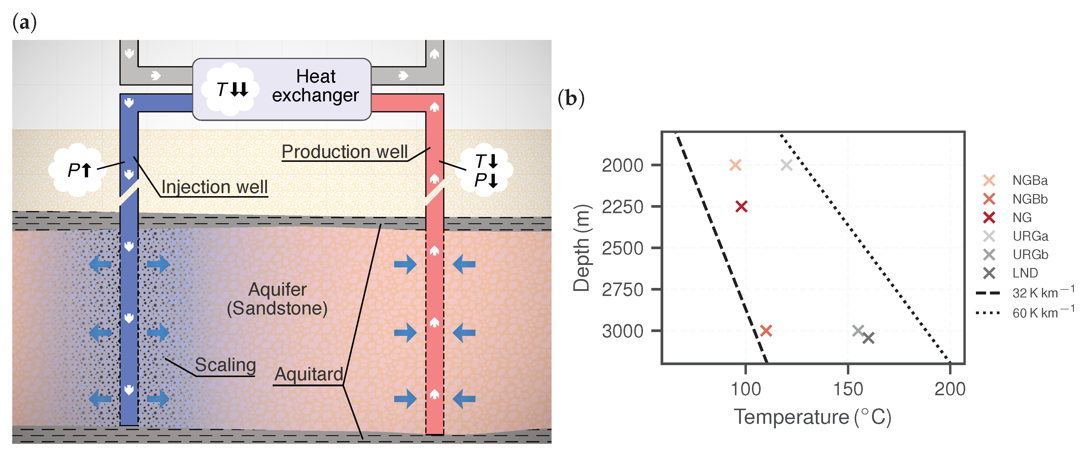
Figure 1. (a) Schematic diagram of a geothermal doublet, showing the core technical installations consisting of a production and an injection well, as well as a heat exchanger. Brine temperature (T) and pressure (P) change along the flow path. Scalings at the injection site clog the pores, which results in reduced injectivity. (b) Fluid temperatures at respective depths for the test cases Neustadt-Glewe (NG), Landau (LND) as well as for the hypothetical sites in the North German Basin (NGB) and the Upper Rhine Graben (URG) (Table 1). The dashed line represents the average geothermal gradient for Germany [15].
Water 12 03078 g001
Figure 2. Model predictions of barite solubility using phreeqc and the Pitzer database at ambient/vapour pressure (solid lines) and 50 MPa (dashed lines) for various temperatures and NaCl -contents. The markers represent experimental values from Blount [16] (circles) and Templeton [17] (crosses).
Water 12 03078 g002
Figure 3. Kinetic rate constant for barite bulk precipitation as a function of temperature and ionic strength (Equation (6)). The dots represent experimental data from Zhen-Wu et al. [32].
Water 12 03078 g003
Figure 4. Dimensionless cases for the radial diverging flow scheme with Damköhler number (a) ranging 0–1 (solid), 0–10 (dashed) and 0–100 (dash-dotted) along the normalised horizontal flow axis. (b) Corresponding normalised steady-state solute concentration.
Water 12 03078 g004
Figure 5. (a) Barite saturation according to reducing temperature for the various geothermal cases. SR barite = 1 represents equilibrium with respect to barite. (b) The associated precipitation potential in units of millimoles per produced cubic metre of formation fluid. At respective reservoir conditions, the values are zero since equilibrium is assumed to be the initial state. The solid lines assume system pressures ( 1 MPa ) and the dashed lines assume the respective reservoir pressures. The dotted vertical lines indicate the assumed injection temperature ( T inj ).
Water 12 03078 g005
Figure 6. Reactive transport simulation results for the NGB cases. (a,c,e) Distribution of porosity change per year for steady-state. (b,d,f) Resulting relative, effective permeability loss (Equation (14)) based on the porosity–permeability relationship (Equation (13)) over the course of ten years. The lines represent respective scenarios.
Water 12 03078 g006
Figure 7. Reactive transport simulation results for the URG cases. (a,c,e) Distribution of porosity change per year for steady-state. (b,d,f) Resulting relative, effective permeability loss (Equation (14)) based on the porosity–permeability relationship (Equation (13)) over the course of ten years. The lines represent respective scenarios.
Water 12 03078 g007
Figure 8. Effective permeability loss after ten years of injecting barite supersaturated fluids into the reservoir. T is the injection temperature, Q is the flow rate and R is the precipitation rate. Note that the connecting dashed lines are only plotted to help distinguish the cases from each other.
Water 12 03078 g008
Figure 9. Scaling score plotted against injectivity loss per year as calculated from reactive transport simulations for the considered geothermal cases and different scenarios (Table 4). The dashed line is a linear regression without intercept. Using Equation (15) for X score , the slope is 2.89 · 10 5 and R 2 = 0.96 .
Water 12 03078 g009
Table 1. Physicochemical parameters (upper part) and chemical composition (lower part) of the considered geothermal fluids. Measured chemical compositions are taken from given literature and converted from ( mg / L ) to ( M ) using calculated solution densities. Reservoir chemical compositions have been calculated to achieve thermodynamic equilibrium with respect to quartz, barite, anhydrite, celesite and calcite at respective reservoir conditions, using the measured values as the basis. Cl has been additionally adjusted to achieve charge balance.
ParameterUnitNGBa a NGBb a NG b , c URGa a URGb a LND d
MeasuredReservoirMeasuredReservoirMeasuredReservoirMeasuredReservoirMeasuredReservoirMeasuredReservoir
T C 2595251102598251202515525160
P e MPa 0.1200.1300.1230.1200.1300.130
ρ s f kg m 3 11301110119011501150111010501000108010101070996
pH 5.605.336.004.915.205.645.805.665.505.285.155.41
IS M 4.054.006.216.114.504.481.371.322.292.312.052.01
Ba 2 + / SO 4 2 NA3.42 × 10 3 NA2.89 × 10 2 8.33 × 10 3 5.47 × 10 3 NA3.19 × 10 3 NA2.64 × 10 2 6.38 × 10 2 3.62 × 10 2
K + M 2.06 × 10 2 2.06 × 10 2 2.87 × 10 2 2.87 × 10 2 2.24 × 10 2 2.24 × 10 2 7.88 × 10 2 7.88 × 10 2 1.33 × 10 1 1.33 × 10 1 1.06 × 10 1 1.06 × 10 1
Na + 3.083.084.874.873.543.548.94 × 10 1 8.94 × 10 1 1.591.591.271.27
Ca 2 + 2.11 × 10 1 2.15 × 10 1 3.49 × 10 1 3.47 × 10 1 2.33 × 10 1 2.37 × 10 1 1.03 × 10 1 1.04 × 10 1 1.82 × 10 1 1.77 × 10 1 1.99 × 10 1 1.96 × 10 1
Mg 2 + 7.53 × 10 2 7.53 × 10 2 4.61 × 10 2 4.61 × 10 2 6.43 × 10 2 6.43 × 10 2 4.23 × 10 3 4.23 × 10 3 4.29 × 10 3 4.29 × 10 3 3.25 × 10 3 3.25 × 10 3
Sr 2 + 5.53 × 10 3 3.38 × 10 3 8.57 × 10 3 5.70 × 10 3 5.61 × 10 3 3.80 × 10 3 2.58 × 10 3 2.70 × 10 3 4.16 × 10 3 8.83 × 10 3 5.09 × 10 3 1.06 × 10 2
Ba 2 + NA2.71 × 10 5 NA1.30 × 10 4 4.43 × 10 5 3.77 × 10 5 NA1.89 × 10 5 NA9.53 × 10 5 8.69 × 10 5 1.10 × 10 4
Fe 2 + / 3 + 1.73 × 10 3 1.73 × 10 3 2.61 × 10 3 2.61 × 10 3 1.26 × 10 3 1.26 × 10 3 1.84 × 10 3 1.84 × 10 3 3.73 × 10 3 3.73 × 10 3 4.03 × 10 4 4.03 × 10 4
Cl 3.793.675.855.694.194.151.301.182.062.101.881.79
Br 4.04 × 10 3 4.04 × 10 3 6.73 × 10 3 6.73 × 10 3 5.30 × 10 3 5.30 × 10 3 1.29 × 10 3 1.29 × 10 3 2.61 × 10 3 2.61 × 10 3 2.84 × 10 3 2.84 × 10 3
SO 4 2 5.04 × 10 3 7.91 × 10 3 7.58 × 10 3 4.49 × 10 3 5.31 × 10 3 6.89 × 10 3 3.74 × 10 3 5.93 × 10 3 3.26 × 10 3 3.61 × 10 3 1.36 × 10 3 3.02 × 10 3
HCO 3 3.97 × 10 3 3.61 × 10 3 5.97 × 10 3 4.10 × 10 3 7.11 × 10 4 8.32 × 10 4 4.21 × 10 3 4.04 × 10 3 7.69 × 10 3 7.42 × 10 3 4.01 × 10 3 4.14 × 10 3
SiO 2 NA4.15 × 10 4 NA4.25 × 10 4 NA4.16 × 10 4 NA1.09 × 10 3 NA1.89 × 10 3 2.75 × 10 3 2.12 × 10 3
T, temperature; P, pressure; ρ s , solution density; I S , ionic strength; NA, values are not available from sources. The sample names are North German Basin (NGB) and Upper Rhine Graben (URG) at 2000 m (a) and 3000 m (b), respectively, as well as the geothermal sites Neustadt-Glewe (NG) and Landau (LND). a Wolfgramm and Seibt [8]. b Naumann [6]. c Kühn et al. [41]. d Sanjuan et al. [7]. e Down-hole pressure derived from depth (Figure 1). f Calculated iteratively with PHREEQC.
Table 2. Hydraulic parameters of a potential hydrothermal reservoir taken from Franz et al. [52].
r w ( m ) Q ( m 3 h 1 ) K ( mD ) M ( m ) ϕ ( )
0.22100500200.2
r w is the well radius, Q is the flow rate, K is the permeability, M is the aquifer thickness and ϕ is the porosity.
Table 3. Varied parameters in the respective scenarios for a one-at-a-time sensitivity analysis. Decreasing Q and w barite corresponds to decreasing flow velocity and precipitation rate, respectively.
ScenarioParameterValueUnit
T + 10 C T65 C
T 10 C T45 C
Q / 2 Q50 m 3 h 1
R / 10 w barite 0.01
Table 4. Summary of results of the equilibrium calculations and the reactive transport simulations for all considered geothermal cases and scenarios. Further, the developed empirical scaling score X score is shown (Equation (15)).
Scenario n barite m Da Loss X score
Case mmol m 3 1 m 1 year 10 4 mol m year
NGBaBase164.40.0186.1
NGBa T + 10 C 165.60.0187.9
NGBa T 10 C 163.30.0164.7
NGBa Q / 2 168.70.0166.1
NGBa R / 10 160.430.00260.61
NGBbBase872.80.06422
NGBb T + 10 C 873.60.06927
NGBb T 10 C 872.10.05616
NGBb Q / 2 875.60.0622
NGBb R / 10 870.280.012.1
NGBase234.10.0248.3
NG T + 10 C 235.30.02511
NG T 10 C 233.20.0226.4
NG Q / 2 238.20.0228.3
NG R / 10 230.410.00360.83
URGaBase121.60.00571.7
URGa T + 10 C 122.30.00662.4
URGa T 10 C 121.20.00481.2
URGa Q / 2 123.30.00511.7
URGa R / 10 120.160.00080.17
URGbBase741.10.0246.9
URGb T + 10 C 741.40.0299.2
URGb T 10 C 740.790.025.1
URGb Q / 2 742.10.0226.9
URGb R / 10 740.110.00340.69
LNDBase850.80.0226
LND T + 10 C 8510.0267.8
LND T 10 C 850.580.0184.3
LND Q / 2 851.60.026
LND R / 10 850.080.0030.6
T is the injection temperature, Q is the flow rate, R is the precipitation rate, n barite is the total precipitation potential, m Da is the slope of the Damköhler number along the r-axis and Loss represents the relative, effective permeability decrease per year, as in 1 K / K 0 .
Publisher’s Note: MDPI stays neutral with regard to jurisdictional claims in published maps and institutional affiliations.

