Are the Financial Markets Sensitive to Hydrological Risk? Evidence from the Bovespa

Abstract

This research analyzes the BOVESPA stock market response to the worst drought occurred in the last 100 years in Brazil. For this purpose, we conducted a standard event study analysis in order to assess the financial response to such hydrological risk on a sample of seven Brazilian agri-food firms. We found statistically significant negative cumulative average abnormal returns (CAARs) around the drought official announcement for different event windows used. Particularly, the highest impact was obtained for the narrowest temporary window, five days around the event disclosure. Moreover, we also found the drought announcement affects even more negatively those companies that sell perishable products, five out of seven in our sample, versus those selling nonperishable ones by running a two-sample t-test on CAARs. This study brings awareness to the climate change impact into the emerging financial markets and the risk faced by shareholders when investing in the agri-food sector, not only in Brazil but also in other Latin American countries, due to the increasing probability to suffer from droughts.

1. Introduction

Climate change is one of the main risks we are facing worldwide. According to the Intergovernmental Panel on Climate Change [1] “Climate change refers to a change in the state of the climate that can be identified by changes in the mean and/or the variability of its properties and that persists for an extended period, typically decades or longer”. It means a change of climate caused by human activity that modifies the composition of the global atmosphere and is observed over comparable time periods [2]. For the World Bank (WB, henceforth) and Inter−American Development Bank (IDB, henceforth), climate change includes changes in the variability of the weather, these are jointly represented as changes in the extremes of the weather, such as a greater number of rainfall events, bringing floods or droughts [3]. To reinforce this idea, the [1] has pointed out that changes are already occurring not only in terms of frequency and severity of the hydrological events, but also in their geographical location [4]. That is why the United Nations Environment Program [5] initiated an investigation to align the financial system to sustainable development needs. The changes observed are connected to growths in the areas affected by droughts, in the number of events causing floods, and in the duration and intensity of certain kinds of tropical storms. Drought-related disasters are also rising, with 3.5 times as many in the past decade, in comparison with 1970–1979. Moreover, the frequency of heat-related disasters has increased 10-fold compared with the 1970s [6].

In relative terms, drought is defined as a negative pluviometric anomaly, which is intense and of sufficient duration to produce social effects. Droughts are, therefore, natural in origin. The complexity of the phenomenon, the geographical and temporal limits of which are hard to determine, make it difficult to have a consensus on the definition [7,8,9]. In addition, droughts vary depending on the geographical location and the context [10]. The ambiguity of the term also gives rise to certain confusion and overlap between the concepts of drought (temporary and natural), water deficit (temporary and anthropic), and scarcity (permanent and anthropic) [11]. Moreover, we should also take into account an operational definition, used for the development of prevention and mitigation strategies, in order to identify the phenomenon in terms of its frequency, severity, and duration for a given return period [8]. The level of impact of a drought is also related to the ways in which societies manage water resources and in which develop strategies to cope with these events [9].

Within a well-defined spatial and temporal framework, [12] differentiate four categories of droughts: meteorological drought (decrease in rainfall), agricultural drought (reduction in soil humidity), hydrological drought (reduction in the availability of surface and underground water sources), and socioeconomic drought (reduction of water availability with regard to existing demands). Recently, this widely accepted classification has been considered insufficient as it is approached from a human-centered perspective. Thus, a new category named ecological drought has been added to emphasize the ecosystems and ecosystem services consequences of a drought event [13]. However, so far, interest in droughts is usually due to its socioeconomic aspects (impact, damage, loss), which are, in turn, tied to other complex concepts such as vulnerability and perception [14]. Ref. [15] stated that over the next 30 to 90 years, southern Africa, the United States, southern Europe, Brazil, and southeast Asia will suffer from an increasing drought severity. Particularly, it is highlighted that in a world warmer by 4 °C, precipitation is greatly reduced in the Caribbean, Central America, Central Brazil, and Patagonia, between 20% and 40%. It is expected that the drought conditions increase more than 20%. It is estimated that limiting warming to 2 °C will reduce considerably the risk of drought, a 1% increase in days with drought conditions in the Caribbean and a 9% increase in South America.

Some regions in Brazil, particularly the semi−arid north-east, are suffering from continuous droughts; producing devastation to some agricultural, livestock, and industrial producers. The intensification of extreme droughts in Brazil has promoted the interest among natural resource managers, farmers, development practitioners, researchers, and policymakers to understand the extent to which climate change will impact water resources, food production, incomes, and livelihoods [16]. However, the UK Parliamentary Office of Science and Technology and the Stern report [17] point out that one of the main challenges is “convincing” businesses that climate change is actually happening and will impact in their activities [18]. Most of the existing literature focuses on agriculture as the most sensitive economic sector to the correlated risks tied to natural disasters, but other sectors are also affected, such as the financial one. In practice, such catastrophic events have led some microcredit providers to ration credit [19] or to restructure loans before they have occurred.

In this regard, a useful tool to show the economic impact on different listed companies or sectors is through conducting an event study analysis. In this paper, we attempt to analyze the financial perceptions on hydrological risk, particularly caused by the recent, most severe drought registered in the past 50 years in Brazil. For this purpose, we examine the reaction of the Brazilian agri-food sector, listed in the BOVESPA [20] stock market.

The research is structured as follows. The next section, corresponding to Section 2, explains the data and sample. Section 3 explains the methodological approach. Section 4 develops the research design, Section 5 presents our main findings, and Section 6 summarizes the main conclusions.

2. Literature Review

Ref. [21] analyzed the impact of earthquake affecting the Umbria region in Central Italy (1997) on the tourism sector. By using an event study, they found a reduction of arrivals through the whole event window, particularly evident in the Assisi district where the “missing arrivals” exceeded by 50% the value forecasted by the model for that period. Ref. [22] studied the impact of Hurricane Floyd on the market value of insurance firms, determining how financial markets reacted to changing news about the storm’s characteristics through the insurer stock prices. They demonstrated that the market value of insurance firms is significantly affected by such catastrophic events; however, this effect is not constant, nor is it always negative on each day of the cycle. Ref. [23] also ran an event study to assess the impact of the tsunami in the financial markets by using the CAPM (Capital Asset Pricing Model); the analysis shows that stock markets were almost insensitive to this event. They highlighted a general increase in the long-term market risk of thirteen industrial portfolios in four countries that were directly affected. They conclude that there was no major wealth destruction for equity investors as a result of the Boxing Day tsunami, in line with the findings of [24]. Ref. [25,26], postulate that rare and extreme events influence financial markets’ risk premiums. Finally, they believe that the observed effects are more likely to involve region-specific issues, as shown by [27,28]. Ref. [29] analyzed the impact of the oil spills disasters on the corporate reputation of a sample of oil and gas companies, listed on New York Stock Exchage (NYSE). By using an event study, they demonstrated that reputational risk arises depending on the investors’ perception that the company may incur losses in the future as a result of a possible negligence concerning such environmental disasters. Ref. [30] examined the US market reaction to ISO 14001 certification announcements. They carried out an event study analysis on a sample of 140 announcements, in order to assess if the new deal between companies and environmental care could be particular important for shareholders, more specifically, in manufacturing, finding a negative impact on the stock returns. Moreover, they proved that the shareholder wealth was reduced due to these certifications announcements. Ref. [31] used an event study method to assess how the stocks of listed companies reacted before and after announcing their partnership with the Unites States Environmental Protection Agency (USEPA) Climate Leaders program. The results suggest that these firms’ public announcements of joining the USEPA Climate Leaders partnership did not have a positive impact on stock returns. While this study demonstrated no immediate financial benefit from the practices implemented by these firms to reduce their greenhouse gas emissions, it may still bode well for long-term corporate earnings and attractiveness to investors, in line with the findings of [32]. Ref. [33] analyzed the stock market’s reaction to information disclosure of environmental violation events (henceforth, EVEs). Using the methodology of event study, daily abnormal return (AR) and accumulative abnormal return (CAR) are calculated within different event windows in order to examine the extent to which the stock market responds to such EVEs. Their findings revealed that the average reduction in market value is much lower than the estimated changes in market value for similar events in other countries, demonstrating that the negative environmental events of Chinese listed companies currently have a weak impact on the stock market. The authors think it is due to the weak implementation effectiveness of the Chinese law system, making investors have a low expectation of the legal impact of such events in the future. This study raises the concerns of environmental conservation to the emerging economies and highlights the need to strengthen up government regulations as well as to improve the effectiveness of law implementation and penalty. To our knowledge, the literature on the effects of droughts on financial markets is almost nonexistent, so this paper contributes to enrich the existing literature of natural disasters (earthquake, tsunamis, hurricanes, floods, etc.).

3. Data and Sample

We have selected some of the companies listed in the industrial index (INDX) of the Brazilian stock market (BOVESPA). This index is formed by 150 companies; most of the important ones, in terms of market capitalization, belong to the agri-industrial and livestock sector and the segment of processed food, which are sensitive to the potential consequences of the drought events. The sample is presented in

Table 1. Sample of agri-food companies.

Ticker	Company	Weight (%)	Main Activity
BRFS3	BRF SA	20	Operational holding: frozen foods: meat and derivatives.
JBSS3	JBS	7.56	Frozen foods: meat and derivatives.
CSAN3	COSAN	1.6	Sugar production, alcohol, ethanol, combustible distribution
MDIA3	M.DIASBRANCO	1.11	Production and sale of wheat flour, sponge cakes, margarine, snacks, etc.
MRFG3	MARFRIG	0.85	Production and distribution of meats and derivatives.
SMTO3	SAO MARTINHO	0.71	Production and sale of sugar and derivatives.
BEEF3	MINERVA	0.4	Production and sale of pork meat, poultry, etc.

The percentages represent the participation weight in the BOVESPA stock market index, being the BRF SA the most representative stock with 20% out of the total weight.

:

Brazil is the third-largest agricultural exporter in the world and one of the major producers of soybeans, sugar, orange juice, maize, cotton, chicken, meat, and pigs, representing approximately 6% of the country′s GDP. Although the total agricultural land area has remained stable since the mid-seventies, production has increased by nearly 300% due to technological innovation. However, the severe drought (2015) that occurred in the north-east is considered one of the worst in the past 100 years [34], in terms of water availability. On 3 February 2015, the Food and Agriculture Organization’s (FAO) Chairman, Ms. Jose Graziano da Silva, announced officially the drought declaration and its consequences for the agricultural sector (see

Table 2. Event description. Source: LexisNexis^® Academic.

Event	Date	Operational Loss	Event Description
FAOAnnouncement	3 February 2015	$4300 MM	Brazil risks a massive loss of crops of all kinds of agricultural products, which will generate an increase in prices in the next months.

).

In order to run the event study analysis, we have selected all companies belonging to the processed food segment in the industrial index of BOVESPA. The daily stock prices, the market value, and the index quotes have been obtained from Thomson Reuters Data Stream. A detailed description of the event has been collected from Reuters verified via LexisNexis^® Academic.

4. Methodological Background

Originally introduced by [35,36] in two respective seminal papers, the use of event studies has become widespread in recent financial and accounting research. The event study methodology is based on the Efficient Market Hipothesis [37] that states that asset prices reflect all available information. If markets are efficient then new information is reflected quickly into market prices. Thus, stock prices trade at their fair value. There are three levels of market efficiency:

• Weak-form efficiency: stock prices reflect all historical information published.
• Semi-strong-form efficiency: stock prices fully reflect all past public information as well as recent public information available.
• Strong-form efficiency: stock prices reflect public and unpublicized or “insider” information.

Under the Efficient Market Hipothesis (EMH), any piece of information regarding the firm is supposed to be reflected in the stock prices. Conceptually, event study technique differentiates between the expected returns obtained in the case the event would not have occurred—normal returns, NR—and the returns arising from the event—abnormal returns, AR [29].

Thus, the abnormal return $A{R}_{it}$ is calculated as the difference between the actual return $R_{it}$ of a stock and the normal or expected return $N{R}_{it}$:

$$A{R}_{it } = R_{it}- N{R}_{it}$$

(1)

The normal returns are calculated following the market model [38] as a benchmark. Thus, the normal or expected returns of stock “i” on day “t” are estimated by ordinary least squares (OLS) as follows:

$$N{R}_{it}=\widehat{{\alpha }_i}+\widehat{{\beta }_i}{R}_{mt}$$

(2)

where

• $N{R}_{it}$ the normal return of a stock “i” is at time “t”.
• $R_{mt}$ is the market index;
• $\widehat{{\alpha }_i}$ and $\widehat{{\beta }_i}$ are the parameters estimated by OLS, using 250 trading days prior to the event window.

According to [39], and assuming there are $N$ listed firms in the sample, we can draw a matrix of abnormal returns, denoted by ∑, as

$${\displaystyle \sum } = \left(\begin{array}{ccc}A{R}_{1,T_1}& \dots & A{R}_{N,T_1}\\ ⋮& \cdots & ⋮\\ A{R}_{1,0}& \dots & A{R}_{N,0}\\ ⋮& \cdots & ⋮\\ A{R}_{1,T_2}& \dots & A{R}_{N,T_2}\end{array}\right)$$

(3)

Each column of this matrix represents a time series of abnormal returns for firm “i”, whereas each row is a cross-section of abnormal returns for each day within the event window ($T_1$, $T_2$). In order to examine the stock reactions around events, each firm’s return data could be analyzed separately. Such analysis is usually improved by averaging the information over the whole sample, given rise to the average abnormal return (AAR):

$$AAR=\frac{1}{N}{{\displaystyle \sum }}_{\mathrm{i}=1}^{\mathrm{N}}A{R}_{it}$$

(4)

Ref. [40] also suggest studying the cumulative abnormal returns (CAR), calculated within the event window, by aggregating $A{R}_{it}$ from $T_1$ to $T_2$:

$$CA{R}_i={\displaystyle \sum }_{t =T_1}^{T_2}A{R}_{it}$$

(5)

Finally, in event studies,$CA{R}_i$’s usually aggregated over the sample cross-section, giving rise to the cumulative average abnormal returns (CAAR):

$$CAAR =\frac{1}{N}{\displaystyle \sum }_{i =1}^{N}CA{R}_i$$

(6)

The last step of the event study methodology is to test the statistical significance of the observed stock prices changes in order to assess they are not random. For this purpose, we carry out both parametric and nonparametric tests following [39,40,41]. Parametric test statistics are based on a standard t-test of difference between two means. Since nonparametric tests do not rely on the assumption of normality, they are more reliable than the parametric ones.

5. Research Design

For designing this research, we have defined three event windows, including the event date, E1(−40,+40), E2(−20,+20) and E3(−5,+5), that is, from 5, 20, and 40 days, before and after, the drought announcement; in other words, 81, 41, and 21 days for each event window, respectively. Existing research shows that shorter event periods provide better and more accurate estimations of the impact of the disclosures on the stock prices since the likelihood of confounding factors not related to the event decrease. Later, we estimated the abnormal returns for each particular event window as well as the corresponding cumulative abnormal returns for the sample of agri-food firms.

The first step was to calculate both the sample daily stock returns and the Brazilian market index (BOVESPA) returns by applying natural logarithm [42,43]:

$$R_{it}= ln\left(\frac{P_{it}}{P_{it-1}}\right)$$

(7)

where

• $P_{it}$ is the price of the firm’s stock $i$ at day $t$.
• $P_{it-1}$ is the price of the firm’s stock $i$ the day before.

Once the observed returns for both the sample companies and the BOVESPA index were calculated, we estimated the corresponding expected returns by using ordinary least squares for 250 trading days, about a year of trading prior to the event window (see Equation (2)). Reaching this point, we calculated the stock’s abnormal returns (AR_it) following the Equation (1).

In

Table 3. Average abnormal returns (AAR) for Brazilian companies.

Event Window	BRFS3	JBSS3	CSAN3	MDIA3	MRFG3	SMTO3	BEEF3	Average
E(−40,+40)	−0.3%	0.28%	−0.09%	−0.03%	−0.50%	−0.13%	−0.38%	−0.14%
E(−20,+20)	−0.09%	0.17%	0.02%	−0.06%	−0.71%	−0.05%	−0.10%	−0.12%
E(−5,+5)	0.20%	−0.04%	−0.19%	−0.48%	−0.76%	−0.56%	−0.41%	−0.32%

, we summarize the average of abnormal returns for each Brazilian company within the corresponding event window. We find much higher negative returns in the shorter event window E(−5,+5) in comparison with the largest ones. In the last column of the table, we calculated the mean of the abnormal returns for the whole sample in each event window. Note that the mean for E(−5,+5) is around double that for the E(−20,+20) and E(−40,+40), indicating the higher impact of the event in the very short term.

Then, we drew the ∑ matrix (see Equation (3)) for the whole sample, which summarizes the abnormal returns of the seven companies analyzed for each event window. Moreover, we have also calculated the average abnormal return (AAR), the cumulative abnormal returns (CAR), and the cumulative average abnormal returns (CAAR), following the Equations (4)–(6), respectively.

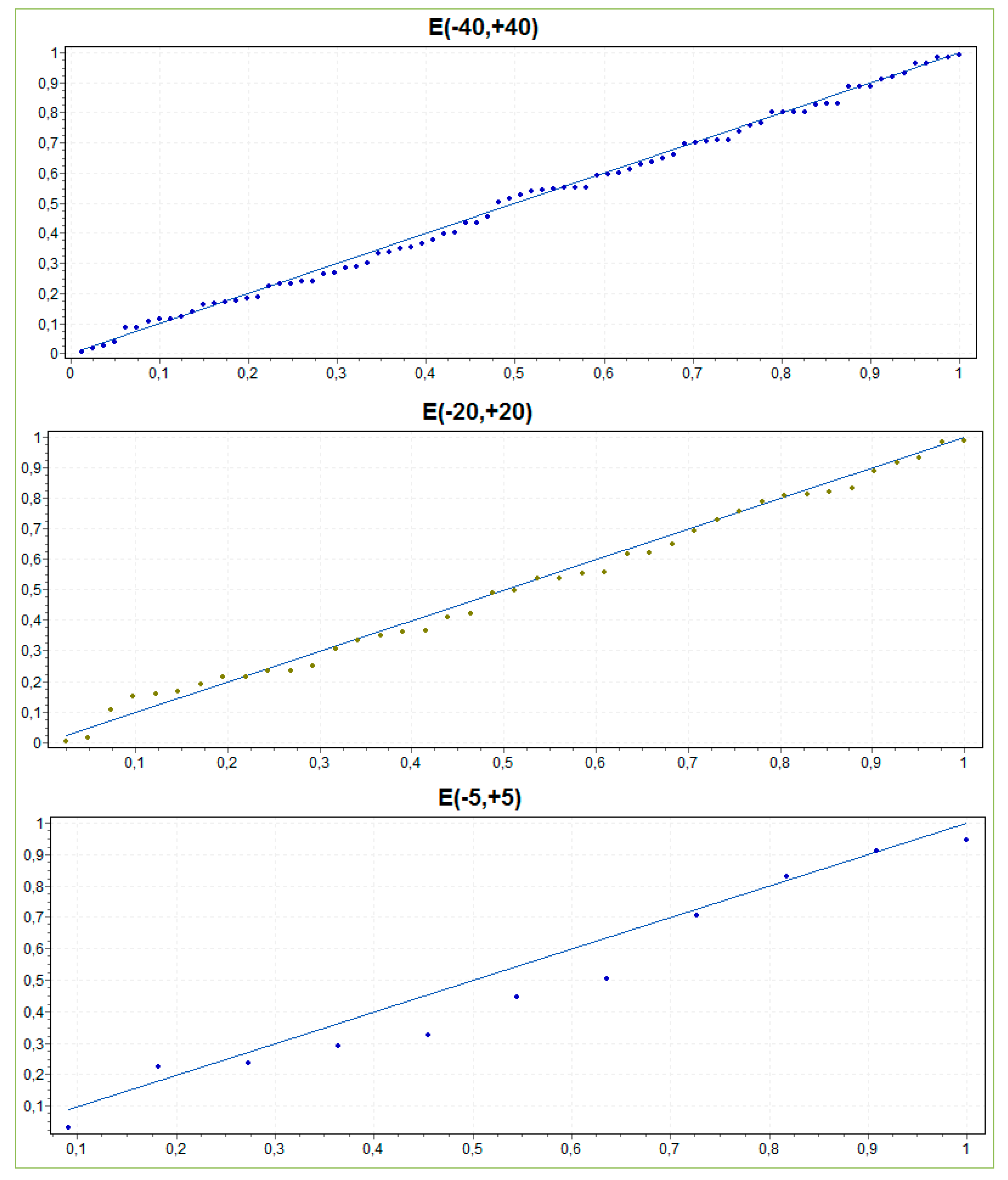
At this point, we ran a normality test by using Anderson−Darling (AD) test since it requires smaller samples than the Kolmogorov–Smirnov (KS) test to achieve sufficient statistical power [44]. As in our case seven companies were analyzed, the Anderson−Darling test is then more appropriate. Therefore, we have conducted the AD test on the average abnormal return (AAR) for the event windows E(−40,+40), E(−20,+20), and E(−5,+5), and the normality assumption is not rejected, as the following Probability-Probability (P-P) plots illustrate (see Figure 1):

After checking the normality assumption, it was time to test the significance of the cumulative abnormal returns. For this purpose, we first applied the parametric t-test [45,46,47,48]. The traditional t-test relies on the normality assumption of abnormal returns. The null hypothesis is that stock prices do not react to the drought announcement. Assuming that the abnormal returns are independent and identically distributed, the statistic follows a Student’s distribution.

The use of nonparametric test provides a double-check of the robustness of the parametric test results [49]. In this sense, we used both the sign test [50,51,52] and the Wilcoxon test [53,54]. The sign test is a binomial test which calibrates if the frequency of abnormal positive residuals is equal to 50%. To apply this test, we calculated the proportion of values in the sample that shed no negative AR’s under the null hypothesis. The null value is estimated as the average fraction of stocks with no negative AR′s in the estimation period. If AR’s are independent, under the null hypothesis, the number of positive abnormal return values follows a binomial distribution. The Wilcoxon test considers both the sign and the magnitude of abnormal returns. This test assumes that none of the absolute values are the same and each is non-zero. Under the null hypothesis, the probability of positive and negative abnormal returns is equal.

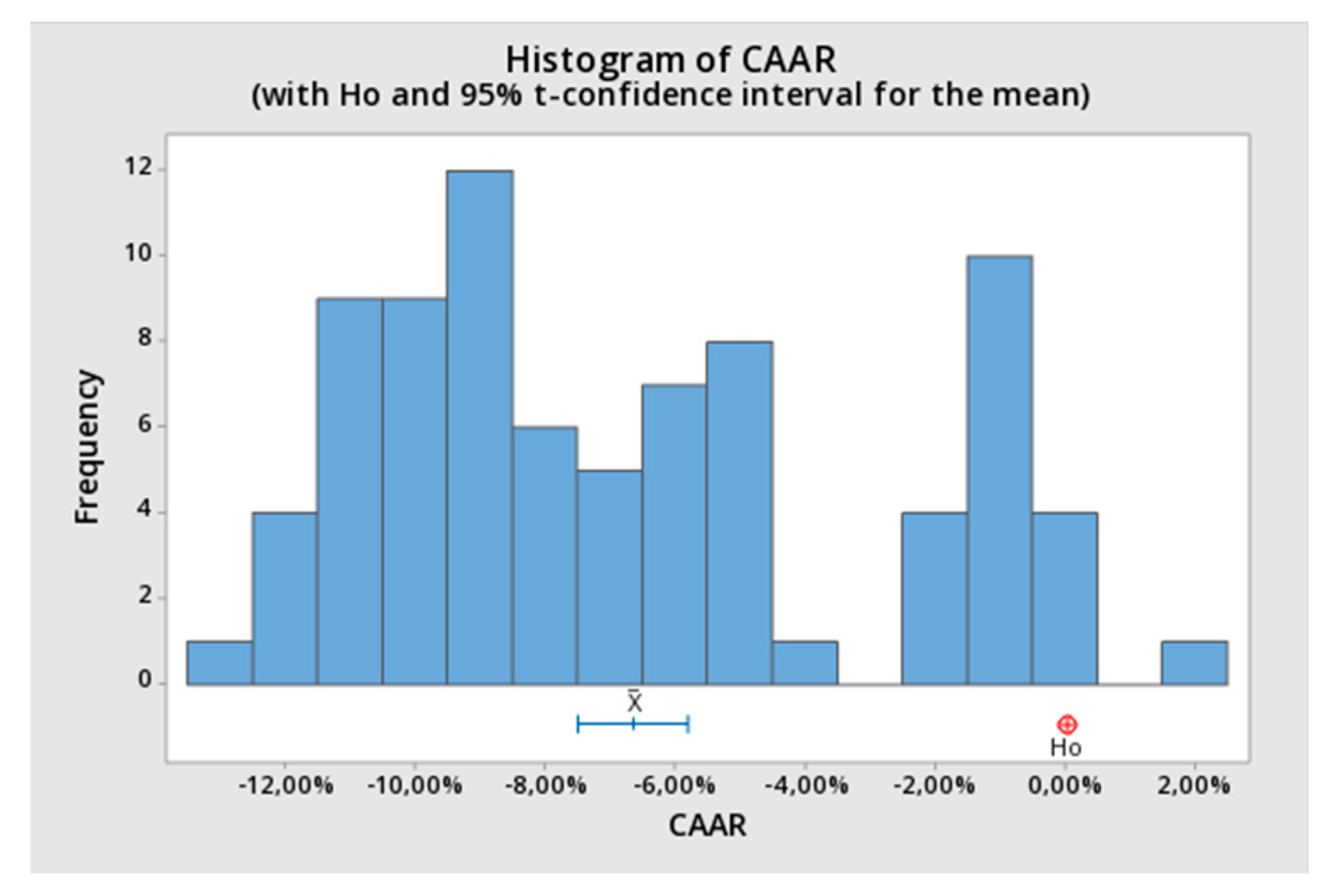
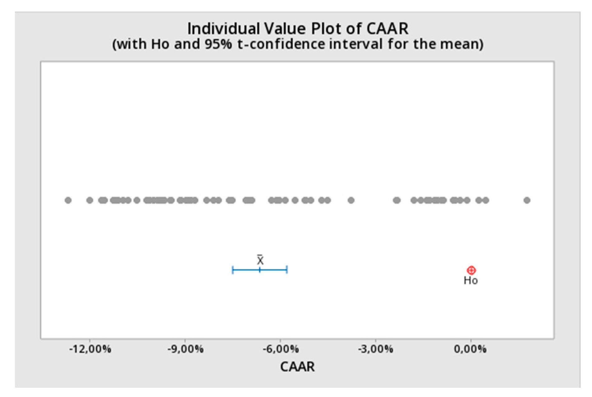
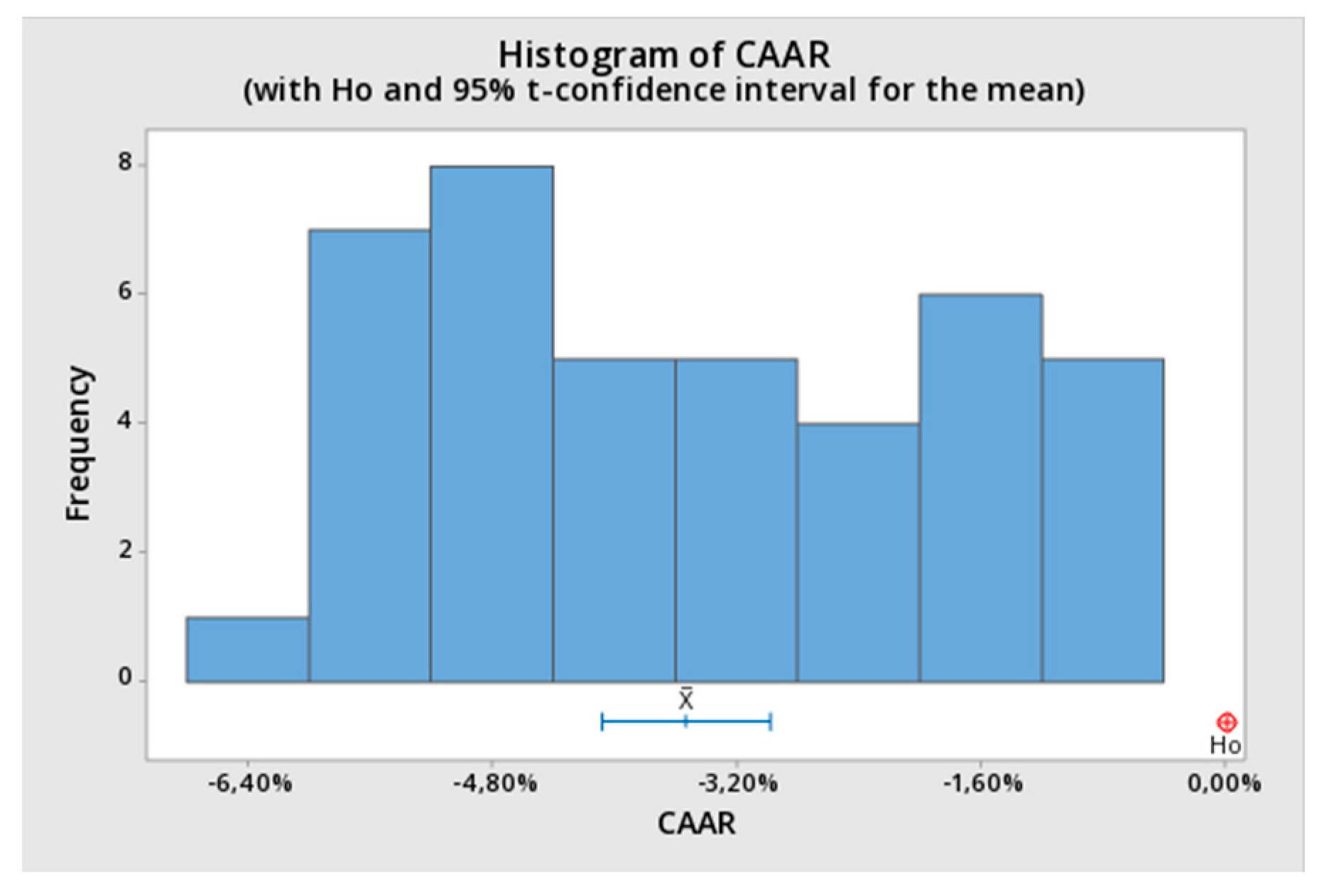
6. Finding and Results

As mentioned in the previous Section, a parametric test (t-test) was first conducted to study the reactions of the agri-food Brazilian companies to the draught announcement for the three event windows, E(−40,+40), E(−20,+20), and E(−5,+5). The idea behind this is to test if the mean of the CAARs is equal (null hypothesis, H₀) or different to zero (H₁), that is

$$H_0 = E\left(\mathrm{CAAR}\right) = 0$$

(8)

$$H_1 = E\left(\mathrm{CAAR}\right)\ne 0$$

(9)

Table 4. T-test on cumulative average abnormal returns (CAARs).

Variable	Mean	t-Value	p-Value	95% CI
CAAR (−5,+5)	−0.01877	−3.22	0.009	(−0.03174; −0.00580)
CAAR (−20,+20)	−0.03529	−13.00	0.000	(−0.04078; −0.02981)
CAAR (−40,+40)	−0.0664	−15.58	0.000	(−0.07488; −0.05791)

summarizes the results obtained from the parametric t-test:

Setting the specific confidence level (95%), we observe that the p-values are smaller than our choice of significance α (0.05), so we can reject the null hypothesis H₀, accepting H₁ for all the event windows. As a consequence, we find a statistically significant abnormal behavior produced by the draught announcement. 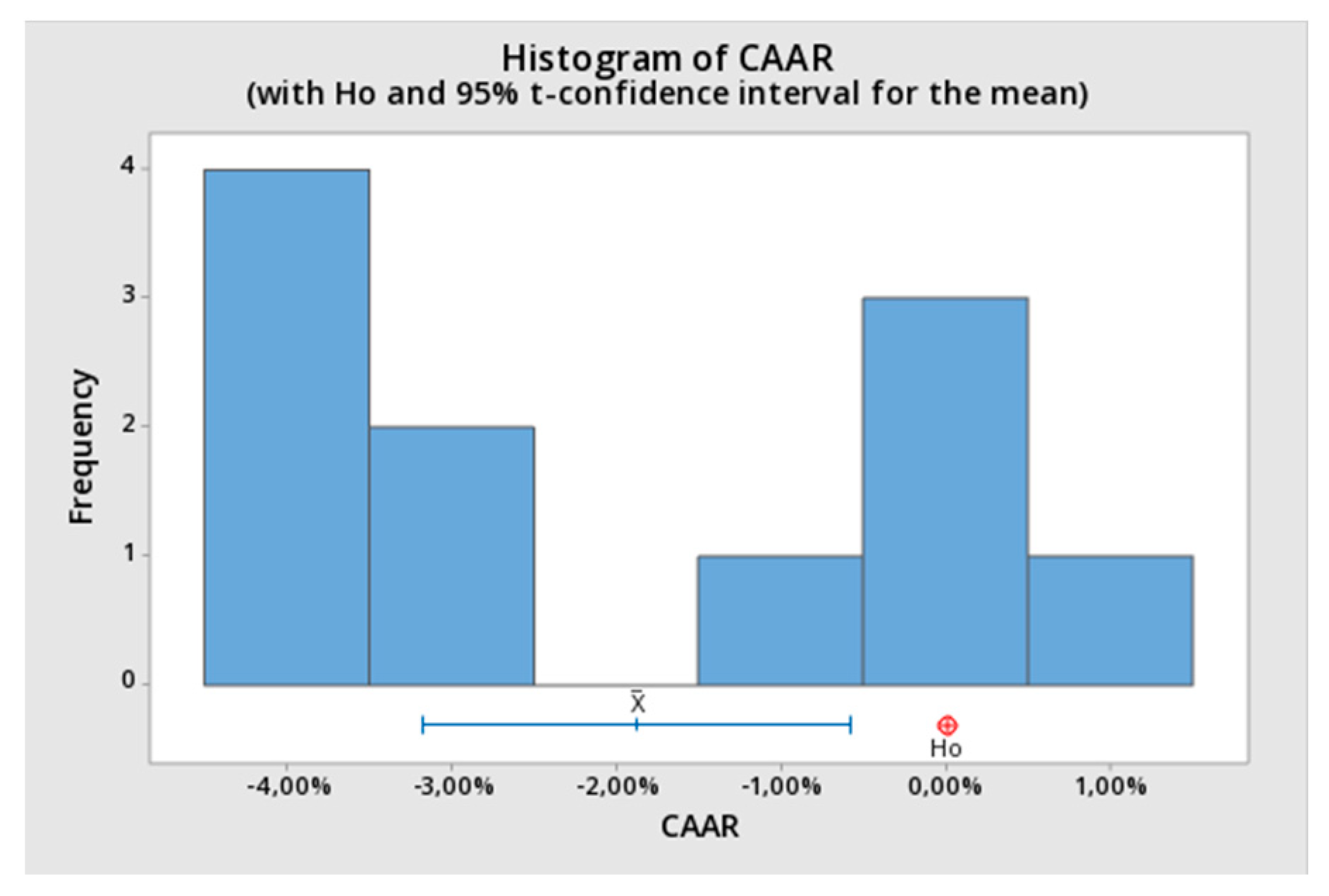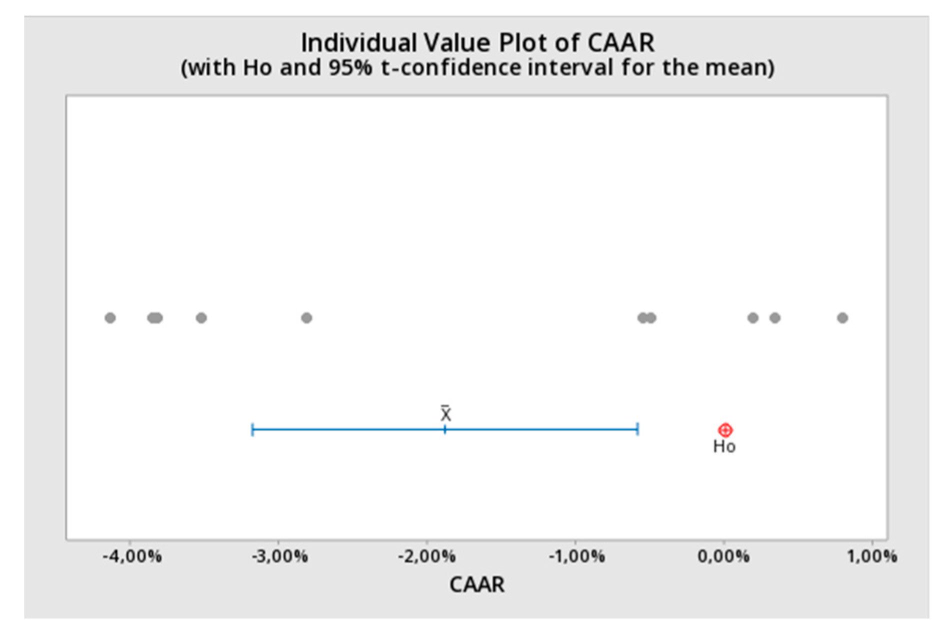In the following Figure 2, Figure 3, Figure 4, Figure 5, Figure 6 and Figure 7, we illustrate those results of the t-test (95%) by using the corresponding histograms and P-P plots. It is easy to infer that the null hypothesis, represented by the dot H₀, is rejected for all the estimation windows, since the mean of CAARs is located far from it.

After applying this parametric test, we also conducted two nonparametric tests in order to reinforce our research: The sign test and Wilcoxon test. The results of both tests are shown below, in

Table 5. Sign test on CAAR.

Variable	Median	Achieved Confidence	Confidence Interval		p-Value
			Lower	Upper
CAAR (−5,+5)	−0.02808	93.46%	−0.03816	0.00194	0.027
		95.00%	−0.03819	0.00206
		98.83%	−0.03852	0.00346
CAAR (−20,+20)	−0.03683	94.04%	−0.04879	−0.02584	0.000
		95.00%	−0.0488	−0.02558
		97.25%	−0.04883	−0.02437
CAAR (−40,+40)	−0.07515	92.46%	−0.08821	−0.06133	0.000
		95.00%	−0.08841	−0.06047
		95.45%	−0.08847	−0.06024

for Sign Test and

Table 6. Wilcoxon test on CAAR.

Variable	Median	p-Value	Achieved Confidence	Confidence Interval
				Lower	Upper
CAAR (−5,+5)	−0.0178	0.029	95.5%	−0.0347	−0.0015
CAAR (−20,+20)	−0.035	0.000	95.0%	−0.0414	−0.0297
CAAR (−40,+40)	−0.0677	0.000	95.0%	−0.0787	−0.0572

for Wilcoxon Test, respectively:

When running the sign test, since the statistic is discrete, the specified confidence level (95%) was not always achieved, so, in Table 5, three confidence intervals appear depending on the achievements. Since the p-value is smaller than the significance level α (0.05), we can conclude that the difference between the median and the hypothesized median of CAAR is statistically significant, thus rejecting the null hypothesis H₀.

Following the same reasoning that in the previous test, for the three event windows, the p-value is smaller than the significance level α (0.05), so we also reject the null hypothesis H₀; accepting that the median of CAARs differs from the hypothesized one.

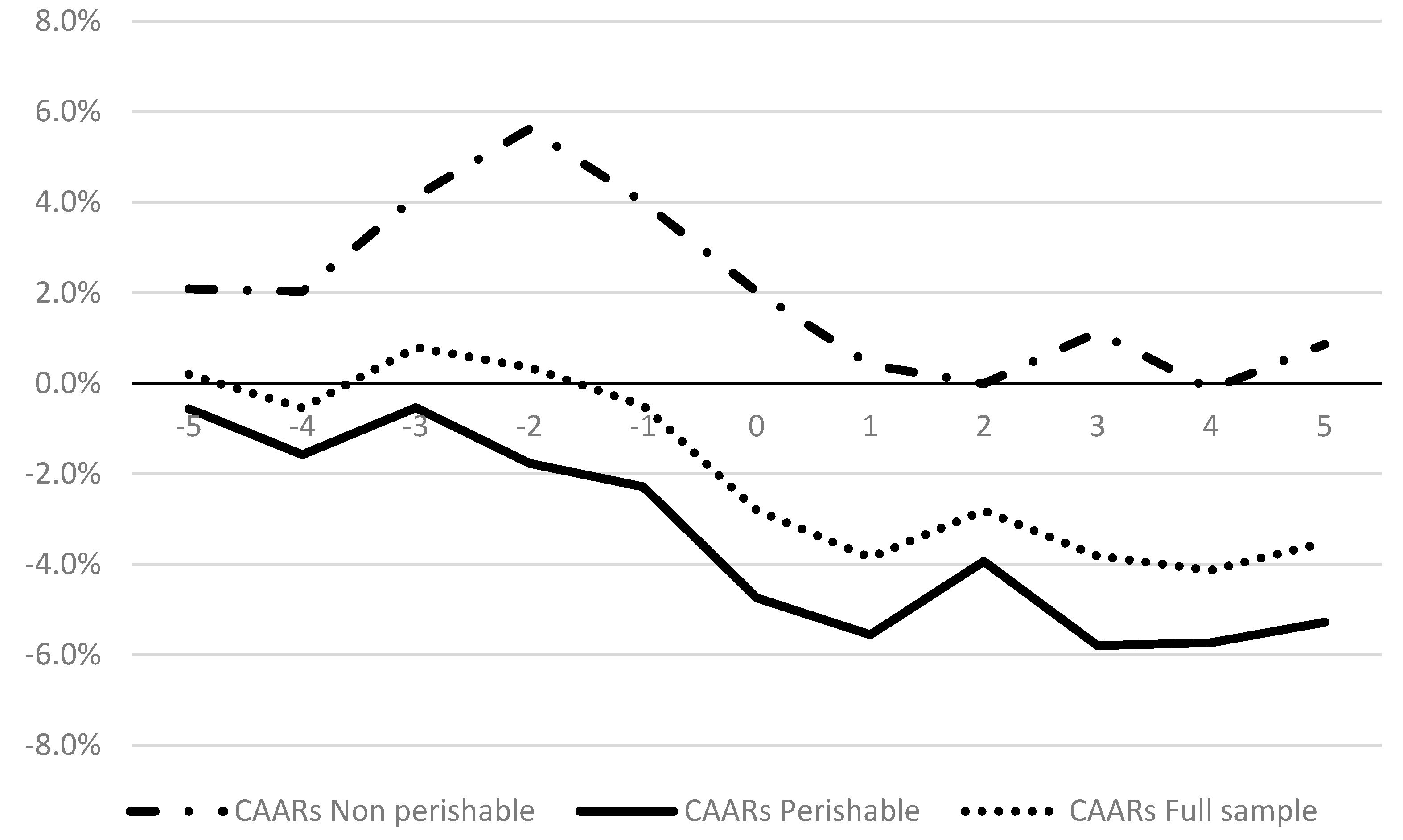
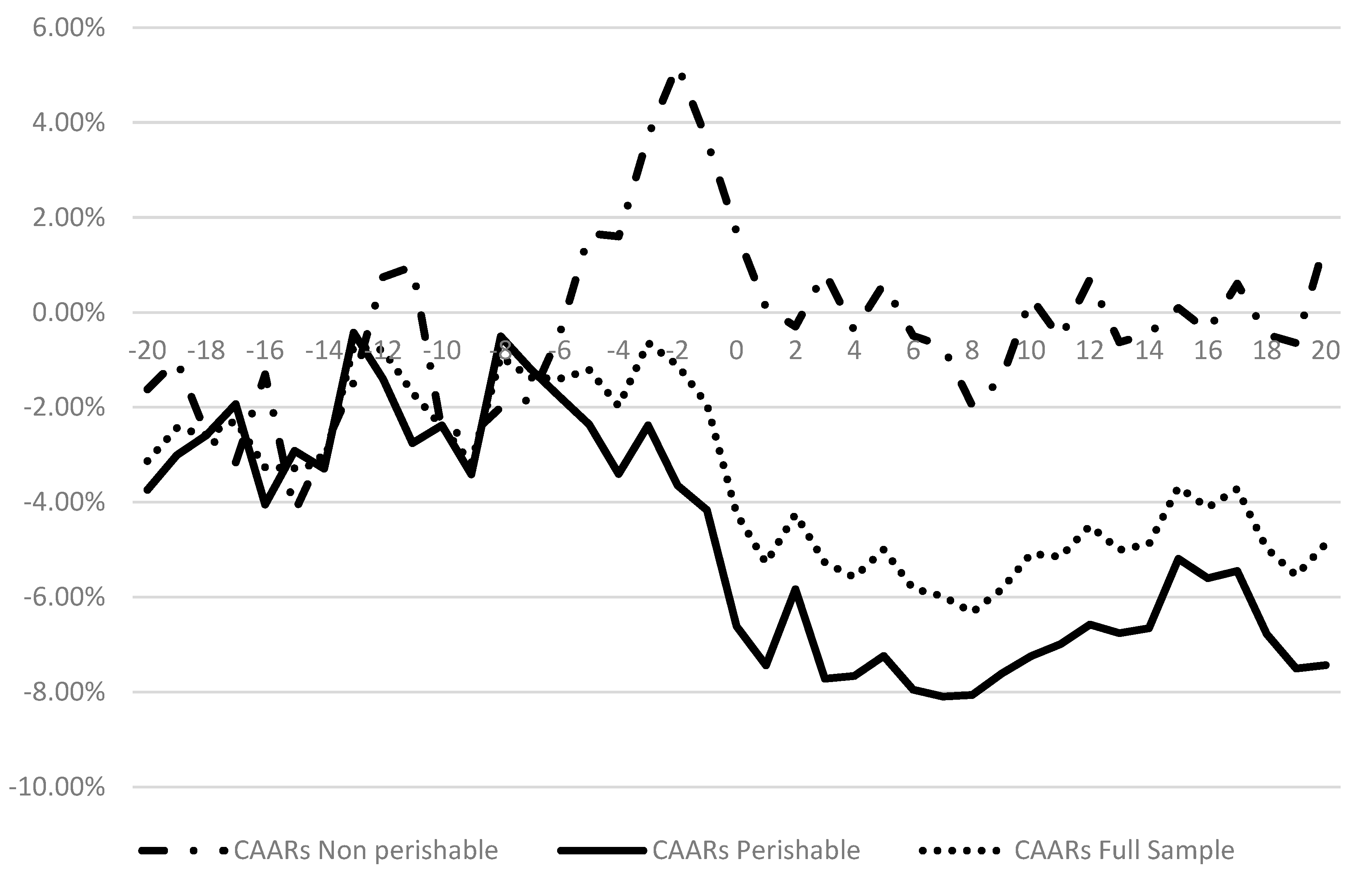
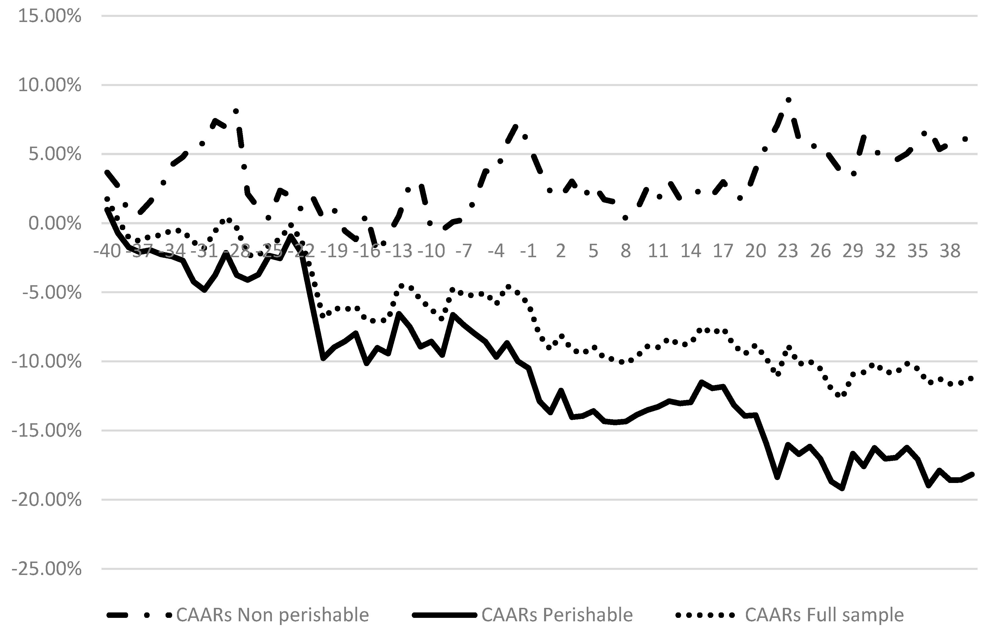
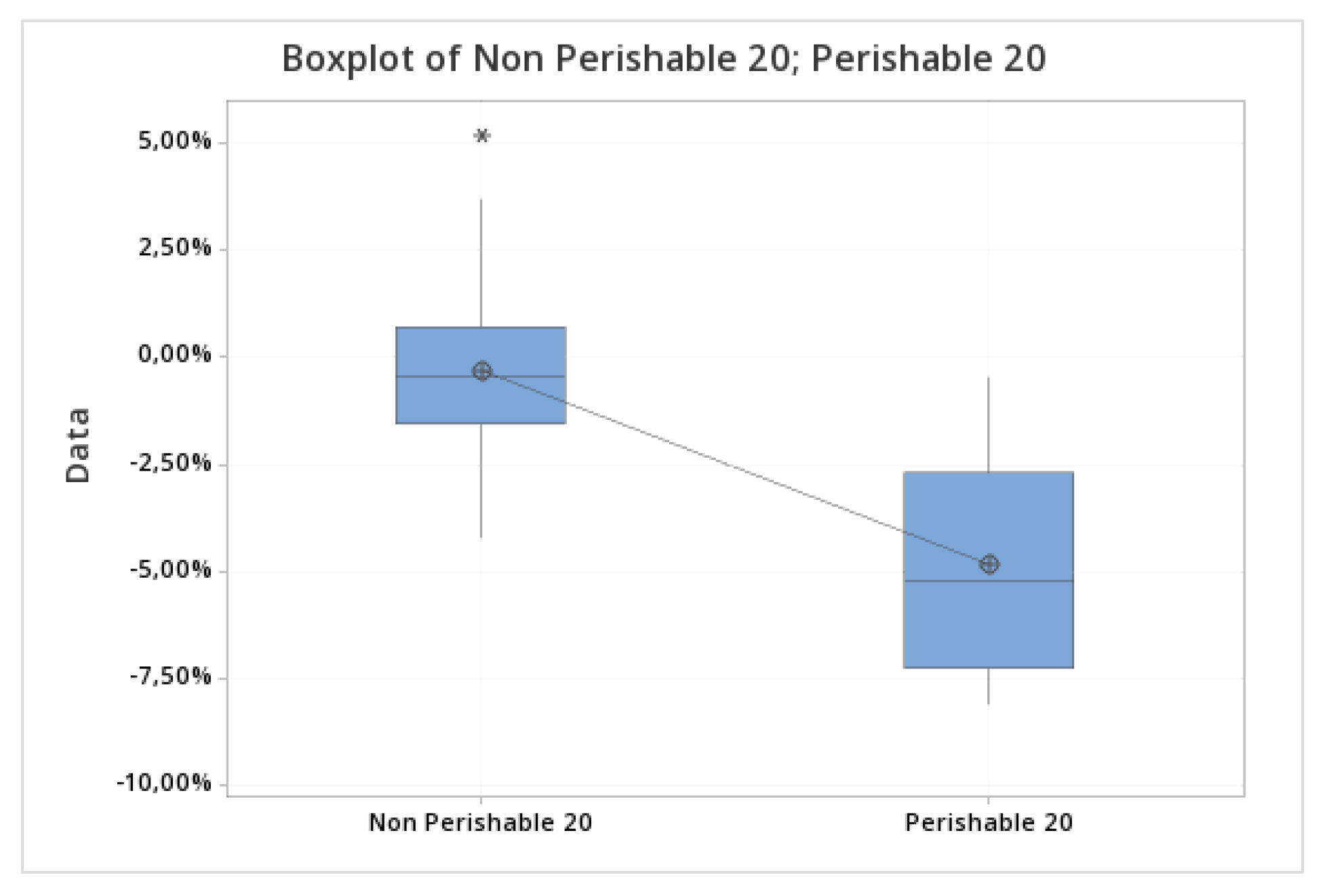
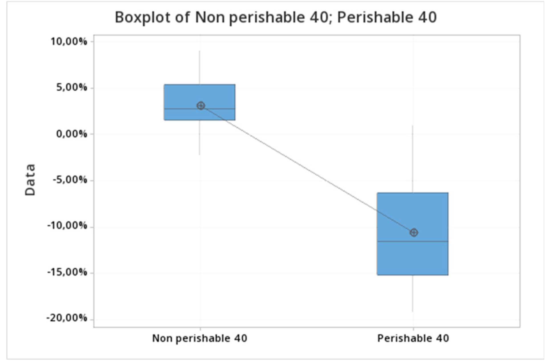
Reaching this point, we split the original sample into two main subsamples, just to check if there was a potential different impact of the drought event between nonperishable (BRFS3 and JBSS3) and perishable firms (CSAN3, MDIA3, MRFG3, SMTO3, BEEF3). In the following charts (see Figure 8, Figure 9 and Figure 10), we have drawn the corresponding CAARs for each subsample, as well as the full sample, to illustrate the existence of higher negative impact on the perishable dataset, independently of the event window used.

From a statistical point of view, in order to compare the different impact of the drought event in the two subsample distributions we focus on the comparison of means. The two-sample t−test [55] was then used to determine whether the two-sample means are equal or not. The null hypothesis is defined as H₀: μ₁ − µ₂ = 0, indicating that the difference between the means, in terms of CAARs, of the two subsamples (nonperishable versus perishable one) is equal to 0. On the contrary, the alternative hypothesis states H₁: μ₁ − µ₁ ≠ 0. In

Table 7. Summary of T-test on CAARs subsamples.

E(−5,+5)	N	Mean	StDev	SE Mean	t-Value	DF	p-Value
CAARs nonperishable	11	0.0201	0.0185	0.0056	6.42	19	0.000
CAARs perishable	11	−0.0344	0.0211	0.0064
E(−20,+20)	N	Mean	StDev	SE Mean	t-Value	DF	p-Value
CAARs nonperishable	41	−0.0029	0.0189	0.003	9.42	75	0.000
CAARs perishable	41	−0.0482	0.0243	0.0038
E(−40,+40)	N	Mean	StDev	SE Mean	t-Value	DF	p-Value
CAARs nonperishable	81	0.0315	0.0245	0.0027	20.17	109	0.000
CAARs perishable	81	−0.1056	0.0561	0.0062

, we summarize the results of the t-test.

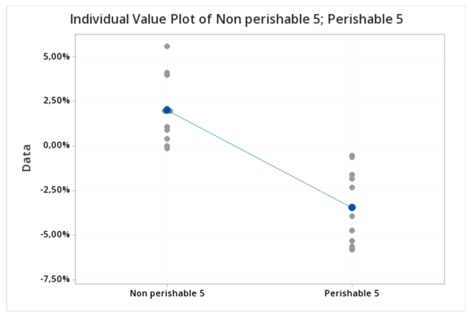
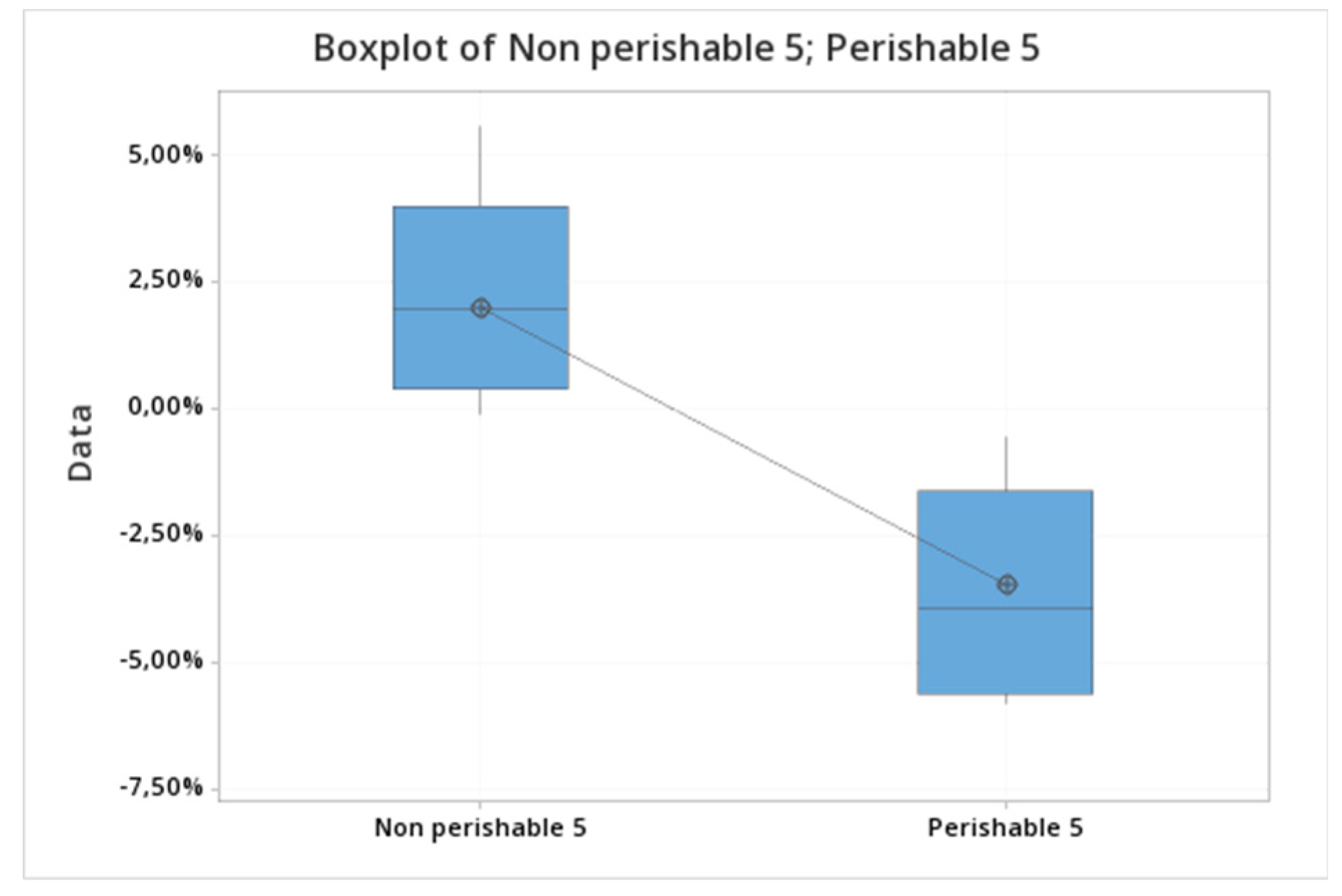
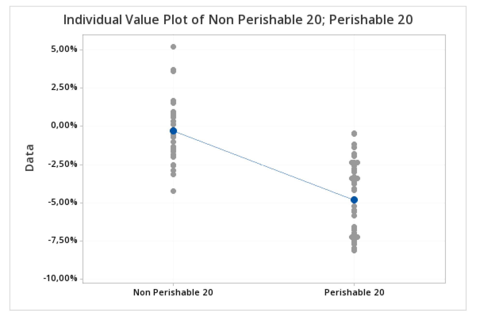
Since the p-value is 0.000, which is less than the significance level of 0.05, we can reject the null hypothesis and conclude that the CAARs of the two subsamples are statistically different for each of the event windows. Note that the mean of CAARs for the perishable subsample remains negative within the three event windows, whereas the mean of CAARs for the nonperishable subsample appears to be positive in two of the three event windows, that is, in E(−5,+5) and E(−40,+40). We can also infer this idea by using the following charts (see Figure 11, Figure 12, Figure 13, Figure 14, Figure 15 and Figure 16):

7. Conclusions

In this paper, we examine how sensitive is the BOVESPA stock market to the worst drought occurred in the last 100 years in Brazil, particularly analyzing the impact of the official announcement on a sample of seven main agri-food listed companies. For this purpose, we carry out a standard short-term event study by using three event windows: ±40, ±20 and ±5 days. After applying both parametric and nonparametric tests, we confirm the existence of statistically significant negative cumulative abnormal returns around the drought official announcement within the three event windows. The highest impact was obtained for the narrowest window, that is, five days before and after the event date, around twice the decline observed for wider windows. Particularly, we observe daily abnormal returns under this mean in three of the companies analyzed, which operate in the frozen food sector, whereas the rest of firms register significant abnormal returns above this threshold. In other words, the impact of the drought announcement affects even more negatively those companies that sell perishable products versus nonperishable ones. To our knowledge, the literature on the effects of droughts on financial markets is almost nonexistent, so this paper contributes to enrich the existing literature of natural disasters (earthquake, tsunamis, hurricanes, floods, etc.). In this regard, we highlight the sensitivity of the BOVESPA stock market to the hydrological risk as well as the complexity of the consequences of climate change in terms of risk perceptions for investors. The results of this study point out the negative impact in terms of cumulative abnormal returns suffered by the agri-food firms as evidence to the next droughts that can be approximate and even intensified in the mid-term. So, shareholders and investors should be aware of the specific risk they face when investing in the agri-food sector, not only in Brazil but also in other Latin American countries, where there is a high degree of probability to see increasing drought severity and extent over the next 30 to 90 years. As with the majority of studies, the current study is subject to limitations since we exclusively focus on the short-term effects of the official drought announcement. In order to capture longer-term effects of the drought, alternative methodologies could be applied, such as the buy-and-hold abnormal return (BHAR) approach and the Jensen’s alpha approach, so this limitation is seen as an opportunity to be addressed in a future research.