Article

Evaluation of an Application of Probabilistic Quantitative Precipitation Forecasts for Flood Forecasting

by
Andrew R. Goenner
1,
Kristie J. Franz
1,
William A. Gallus Jr
1,* and
Brett Roberts
2,3,4
1
Department of Geological and Atmospheric Sciences, Iowa State University, Ames, IA 50011, USA
2
Cooperative Institute for Mesoscale Meteorological Studies, University of Oklahoma, Norman, OK 73019, USA
3
NOAA/OAR/National Severe Storms Laboratory, Norman, OK 73019, USA
4
NOAA/NWS/Storm Prediction Center, Norman 73019, OK, USA
*
Author to whom correspondence should be addressed.
Water 2020, 12(10), 2860; https://doi.org/10.3390/w12102860
Submission received: 17 September 2020 / Revised: 8 October 2020 / Accepted: 12 October 2020 / Published: 14 October 2020

Abstract

:
Probabilistic streamflow forecasts using precipitation derived from ensemble-based Probabilistic Quantitative Precipitation Forecasts (PQPFs) are examined. The PQPFs provide rainfall amounts associated with probabilities of exceedance for all grid points, which are averaged to the watershed scale for input to the operational Sacramento Soil Moisture Accounting hydrologic model to generate probabilistic streamflow predictions. The technique was tested using both the High-Resolution Rapid Refresh Ensemble (HRRRE) and the High-Resolution Ensemble Forecast version 2.0 (HREF) for 11 river basins across the upper Midwest for 109 cases. The resulting discharges associated with low probability of exceedance values were too large; no events were observed having discharges above the 10% exceedance value predicted from the technique applied to both ensembles, and no events were observed having discharges above the 25% exceedance value from the HREF-based forecast. The large differences are due to using the same precipitation exceedance value at all points; it is unlikely that all watershed points would experience the heavy rainfall associated with the 5% probability of exceedance. The technique likely can be improved through calibration of the basin-average precipitation forecasts based on typical distributions of precipitation within the convective systems that dominate warm-season precipitation events or calibration of the resulting probabilistic discharge forecasts.

1. Introduction

Currently, river and stream flood forecasts are usually made using Quantitative Precipitation Estimates (QPEs) [1,2] instead of Quantitative Precipitation Forecasts (QPFs) because large errors can exist in the QPFs. However, because QPE is not available until after the rainfall begins, a hydrologic forecast cannot be made until the precipitation event is underway and the full impact of the event cannot be captured in the streamflow forecast until the rain has ended. This is especially problematic in small river basins where the precipitation event may not have ended before flash flooding has already started to occur. Thus, reliance on QPE for flood forecasting limits the ability of forecasters to predict rapid streamflow changes with much lead time, reducing the time emergency managers have to inform and prepare safety personnel and the general public for potential flooding. Earlier flood warnings could be made if QPFs were used as input to hydrologic models instead of QPEs [3,4,5,6].
One problem in the use of QPFs in hydrologic models is that precipitation forecasts often have substantial errors, especially for warm season rainfall [7,8], which is typically associated with relatively small-scale and intense thunderstorms that have weak large-scale forcing. The small-scale and high intensity of this type of precipitation often makes it particularly challenging to forecast possible resulting flash flooding [9,10], especially because displacement errors in the simulated precipitation systems are common [11,12]. Additionally, the lack of larger-scale forcing means that small-scale forcing mechanisms play a more important role in initiating and sustaining warm-season precipitation systems so that higher resolution is necessary in numerical models to forecast warm-season rainfall. Unfortunately, even models run with fine grids still can struggle to accurately predict small-scale forcing and the resulting precipitation [13,14,15], at least partly because existing limited observational networks that supply the initial conditions for the models may only partially resolve these small-scale mechanisms. In addition, errors can arise from the use of parameterizations for the boundary layer or microphysical processes [16,17,18]. Since it is so challenging to forecast warm-season precipitation events using deterministic model runs, an increasing emphasis has been placed on ensemble forecasting [19,20,21].
Ensemble Prediction Systems (EPSs) assist with forecasting, since EPSs show the uncertainty of an event through probabilistic forecasts [12,22], and the ensemble mean of a variable is often more accurate than values from any individual ensemble member [23,24]. EPSs can use multiple models, different physical parameterizations, and different initial and lateral boundary conditions, thus accounting for many of the uncertainties that can lead to errors in atmospheric models. Werner et al. [25] tested the use of an EPS in streamflow forecasts and discovered that using the mean areal precipitation of the EPS improved the Ranked Probability Skill Score (RPSS) values when compared to the reforecast archived model forecasts. However, Ebert et al. [26] found that the ensemble mean for heavy QPF was usually smaller than that observed due to the averaging process smoothing the extremes from each member, since the locations of predicted heavy rain typically differed among members. The resulting mean QPF field was often unrealistically smooth and light.
Since the precipitation patterns from an ensemble mean may not be physically realistic, a better approach can be to use the individual QPFs from the ensemble members. For example, Davolio et al. [5] showed how QPFs from a multi-model ensemble were useful in generating flood forecasts, although shortcomings with the forecasted timing and shape of the river’s hydrograph were noted. The small scale and intense nature of typical warm-season rainfall aggravate QPF errors associated with both timing and location, such that when input into the hydrologic model, significant errors in watershed-level predictions can occur, especially for small basins [27,28]. Carlberg et al. [29] found that increasing the number of ensemble members by randomly shifting the individual members’ QPF to account for displacement errors led to more skillful probabilistic streamflow forecasts than those of the original EPS. The current operational Hydrological Ensemble Forecasting Service (HEFS) at the National Oceanic and Atmospheric Administration in the United States uses bias correction applied to the ensemble member QPFs that are used as input to create probabilistic streamflow forecasts [30].
Individual member QPFs are commonly used to create probabilistic QPF (PQPF) [31,32], which provides a measure of uncertainty in the rainfall forecasts. Although one could simply assign probabilities at grid points based on the number of members showing precipitation above a threshold, often these forecasts are calibrated by comparing the model forecasts to observations for a period of time to account for systematic biases in the ensembles. In addition, smoothers are often used, which effectively take into account information from nearby grid points [19], possibly mitigating in a small measure displacement errors common to precipitation forecasts. Assuming value is added to the PQPFs by these approaches, the rainfall amounts associated with the PQPFs could be used instead of individual member QPF as input to hydrologic models to create probabilistic streamflow forecasts. Presently, the National Weather Service’s (NWS) North Central River Forecasts Center (NCRFC) generates a probabilistic streamflow forecast using both QPE measurements from the United States Geological Survey and NWS’s Stage IV rainfall data and PQPFs from the NWS Weather Prediction Center using the 5%, 50%, and 95% exceedances. However, they and others who have attempted to use PQPF in similar manners acknowledge that there may be problems in the direct use of PQPF (S. Connely, NCRFC, 2020, personal communication), suggesting that further work is necessary to document how well the technique may work to provide probabilistic streamflow forecasts.
The objective of this study is to determine how skillful probabilistic streamflow forecasts are if they are made using high-resolution ensemble PQPF information directly, with the probability of exceedance rainfall amounts determined from the probabilities that had been assigned to several QPF thresholds as opposed to using member QPFs. Such an approach takes advantage of the fact that statistical techniques such as Gaussian smoothers add value to the ensemble PQPFs. Two operational/quasi-operational high-resolution ensembles are used to compute the rain amounts associated with various probabilities of exceedance in a similar manner to NCRFC’s PQPF forecasts. Then, these values are input into a hydrologic model to test how well this PQPF application works for short-term, warm-season probabilistic streamflow prediction. The streamflow predictions are compared to the operational predictions from the NCRFC.

2. Materials and Methods

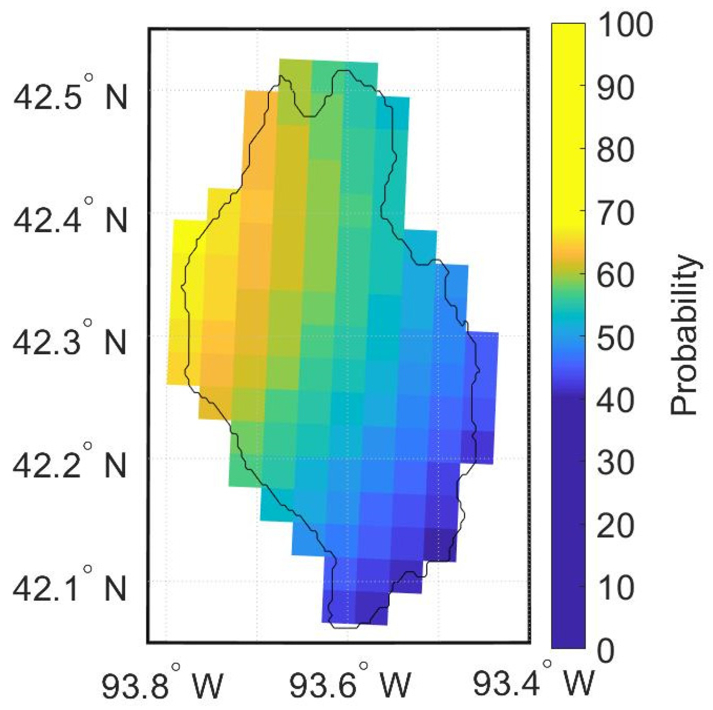
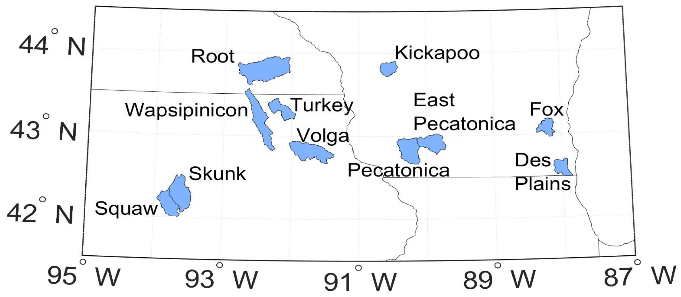
2.1. Study Basins and Case Selection

Eleven basins in Illinois, Iowa, Minnesota, and Wisconsin were selected for this study (Table 1, Figure 1). The basins fall within the forecasting region of the North Central River Forecasting Center (NCRFC). This region is characterized primarily by forested hills and lakes in Minnesota and Wisconsin and plains and farmlands in Illinois and Iowa. The uppermost forecast points on the rivers were selected to eliminate the need to model the inflow of water from upstream locations.
The study period spans 14 June–5 October 2018. To be selected, the streamflow events had to have evidence of a sharp increase in streamflow due to forecasted precipitation, and the observed maximum discharge had to exceed a value higher than the 75% exceedance of the June–September streamflow climatology for that basin based on the available data from the United States Geological Survey (USGS). A total of 109 events were examined across the 11 basins, with 33 of the events exceeding the action stage.

2.2. Precipitation Forecasts

PQPFs from two different operational/quasi-operational high-resolution ensemble systems were tested in this study: The High-Resolution Rapid Refresh Ensemble (HRRRE) of the Earth System Research Laboratory and the High-Resolution Ensemble Forecast version 2.0 (HREF) of the National Centers for Environmental Prediction. The HRRRE consisted of 9 members that ran over a half contiguous United State (CONUS) domain during the summer of 2018, with 3 km horizontal grid spacing (Table 2). The members were created using random variations in the zonal winds, temperature, and water vapor as part of the initial and boundary conditions of the individual members [19]. Random atmospheric perturbations were generated by using the first 36 members of the Global Data Assimilation System (GDAS) formatted to fit on the HRRRE domain. In addition, random perturbations were applied to soil moisture (Trevor Alcott, NOAA, September 2018, personal communication). Each of the members used the same microphysics scheme, Aerosol-Aware Thompson [33], and planetary boundary layer (PBL) scheme, Mellor–Yamada Nakanishi Niino [34]. From the HRRRE, PQPFs were provided for four different 6-hour Accumulated Precipitation (APCP) thresholds: 12.7, 25.4, 50.8, and 76.2 mm. These PQPF values were generated by determining how many of the members exceeded these thresholds at each grid point. This fraction of the members provided a probability value for the APCP thresholds. Afterward, a Gaussian spatial smoother with a radius of 24 km was applied to the specific grid point to limit extreme differences between neighboring grid points [19].
The HREF version 2 was a time-lagged ensemble built using four models [21], the first two being variations of the Weather Research and Forecasting (WRF) model: High-Resolution Window (HRW) National Severe Storms Laboratory model (NSSL) and HRW Advanced Research WRF model (ARW) [35]. Additionally, two variations of the NOAA Environmental Modeling System’s Nonhydrostatic Multiscale Model on the B-grid [36], NMMB, were used: the HRW NMMB and the North American Mesoscale (NAM) Nest forecasting model [37]. In addition to the four members mentioned above, the HREF additionally used four time-lagged members from the same models that were initialized 12 h prior to create an ensemble with 8 members. HREF forecasts were generated twice a day, at 00 and 12 UTC, on a full CONUS domain with a 3 km horizontal grid. The models used different PBL and microphysics schemes. Both NAM members and the HRW NSSL used the Mellor–Yamada Janjic PBL scheme [38], while the HRW–ARW used the Yonsei University PBL scheme [39]. Additionally, the two WRF members used the WRF Single-Moment 6-Class microphysics scheme [40], while the two NAM members used the Ferrier–Aligo scheme [41]. The HRRRE and HREF system configurations are shown in Table 2. The rainfall thresholds for which the HREF generated probability values were 6.4, 12.7, 25.4, and 50.8 mm. HREF PQPF was created in the same way as that of the HRRRE except that the Gaussian smoother used a radius of 40 km [21].
To convert from the four rainfall thresholds in the PQPF to rainfall amounts at the probability of exceedance values of 5%, 10%, 25%, 50%, 75%, 90%, and 95%, a cubic interpolation was performed. These exceedance values were selected to match the probability of exceedance values used by the National Weather Service River Forecast Centers for discharge. Both HRRRE and HREF regularly had predictions of zero probability of occurrence at rainfall amounts equal to or greater than 25.4 mm, thereby reducing the number of unique data points below the necessary three required to complete the cubic interpolation. As a result, it was necessary to expand the number of unique probability values to perform the interpolation. Additionally, it was desired to remove the need to extrapolate beyond the extremes of the PQPF values, as extrapolation can sometimes result in unrealistically large values.
To remove the need for extrapolation, the following two data points were used. First, we define the probability of exceedance as follows: at that value of precipitation or above, a precipitation value of greater than or equal to zero is equated to a probability of exceedance of 100%. As having rainfall values less than 0 is impossible, this assumption closes the range of possible values for the interpolation on the low end, representing the lightest rainfall amount. A second additional point was added at the opposite end of the scale with a probability of exceedance of 0%. This point made use of the maximum rainfall in the Midwest domain from any ensemble member. A value of 0.25 mm was added to this value, making it impossible to find this value inside the domain, thereby justifying a probability of zero for this rainfall amount to close the interpolation of the probability of rainfall exceedance on the upper end of the dataset. With these two extra points, the cubic interpolation could be performed, as shown in Figure 2.
To perform the cubic interpolation, the Piecewise Cubic Hermite Interpolating Polynomial (PCHIP) program was used. Azizan et al. [42] found when comparing PCHIP and a not-a-knot (SPLINE) approach to rainfall interpolation, the SPLINE could produce negative rainfall values, unlike the PCHIP, which stayed positive. Additionally, the computational cost to interpolate with PCHIP was less than with SPLINE or a Modified Akima Cubic Hermite Interpolation (Makima).
For the grid points where no rainfall was predicted in the models, the unique data points were the 100% probability of exceedance of greater than or equal to zero rainfall and the 0% probability of exceedance for the lowest rainfall threshold (6.4 or 12.7 mm). With these grid points, rainfall values of 2.54, 2.29, 1.78, 1.27, 0.76, 0.51, and 0.25 mm were assigned to the 95, 90, 75, 50, 25, 10, and 5 percentiles, respectively. Although these values are arbitrary, the requirement mentioned earlier that observed discharge had to exceed the climatological 75% occurrence for cases to be studied resulted in very few of these dry points being used in the analyses that follow. After precipitation amounts at the different probability of exceedance values were generated, grid points located within basins or in contact with the edges of the basins were averaged to create the basin-averaged precipitation needed as input in the hydrologic model (Figure 3).
To compare the streamflow forecasts made using the PQPF values to a standard representing observations, streamflow forecast model runs also were completed using Stage IV data. Stage IV is a spatially generated quantitative precipitation estimate using both radar and rain gauge measurements. Stage IV precipitation data are created by the River Forecasting Centers at different time intervals, including 1, 6, and 12 h [43]. For this project, the six-hour intervals were selected.

2.3. Hydrologic Prediction Model

Ensemble streamflow forecasts were generated using the spatially lumped Sacramento Soil Moisture Accounting model (SAC-SMA) [44], which is the forecast model used by the NCRFC. Inputs to the SAC-SMA are basin-averaged precipitation and potential evapotranspiration, and the output is basin discharge. The SAC-SMA accounts for water storage and flows in the subsurface using a two-layer soil structure. Each zone has free water storages that account for water drainage by gravity and tension water storages that account for evaporation and transpiration. Evaporation and transpiration are calculated based on the potential evapotranspiration for the time step and the available water in the tension storage. Water inflow to the stream channel is a combination of surface runoff, flow from the upper soil zone, and flow from the lower soil zones, which are computed as a function of soil storages, percolation capacities, and precipitation rates and controlled by 13 primary parameters [45]. Channel inflow is routed using a unit hydrograph to calculate basin discharge.
The model was applied using the 6-hour time step used by the NCRFC for operations. Basin-specific model parameters and unit hydrographs were obtained from the NCRFC for each study basin. The SAC-SMA model states were initialized using a 5-day spin-up period starting from states obtained from the NCRFC for a date 5 days prior to the forecasts followed by precipitation input up to the forecast start date. In initial testing, it was found that a short spin-up period of about 4–8 timesteps was needed for the simulated discharge to reach observed discharges values primarily due to uncertainty in the states of the routing routine.

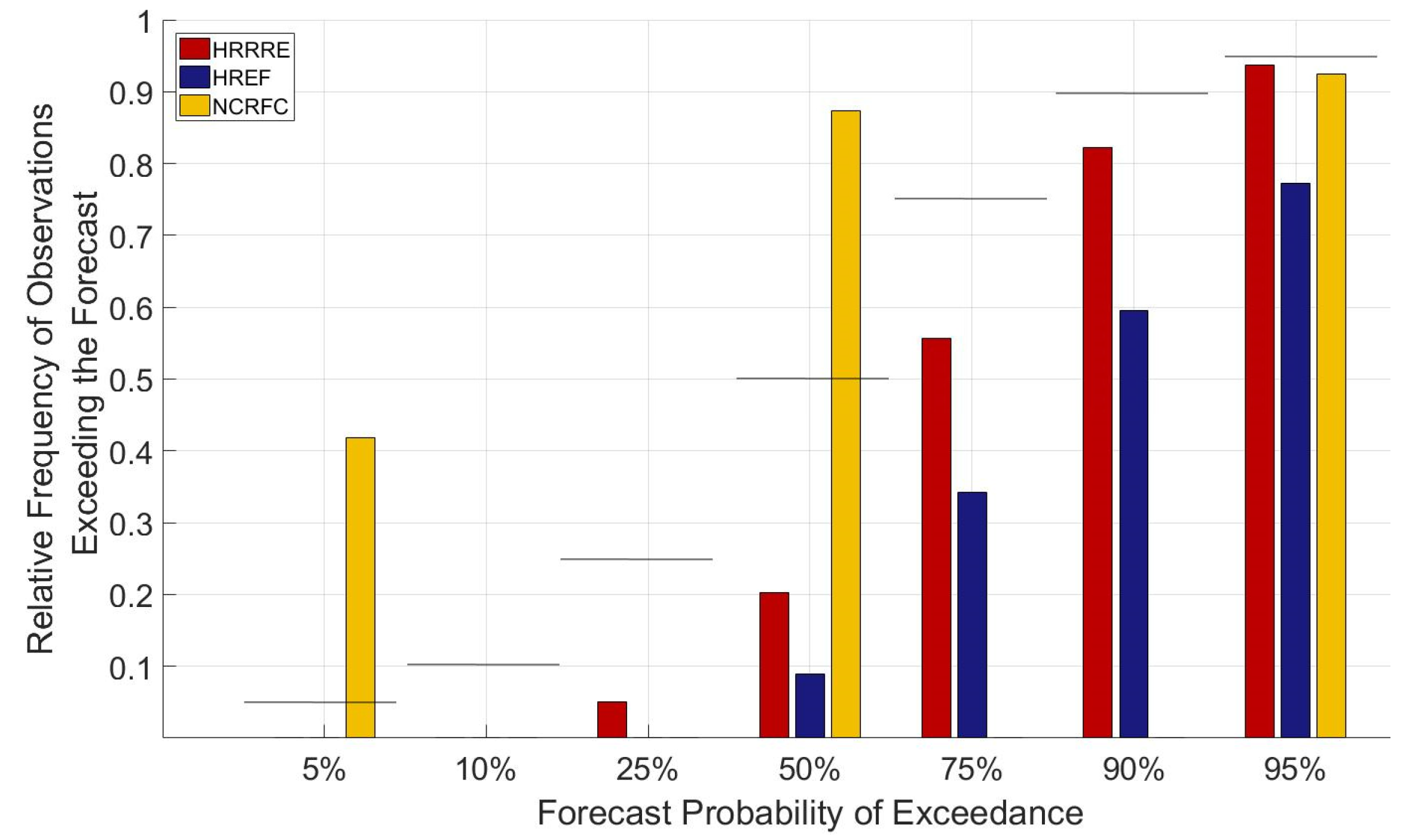
2.4. Forecast Evaluation Statistics
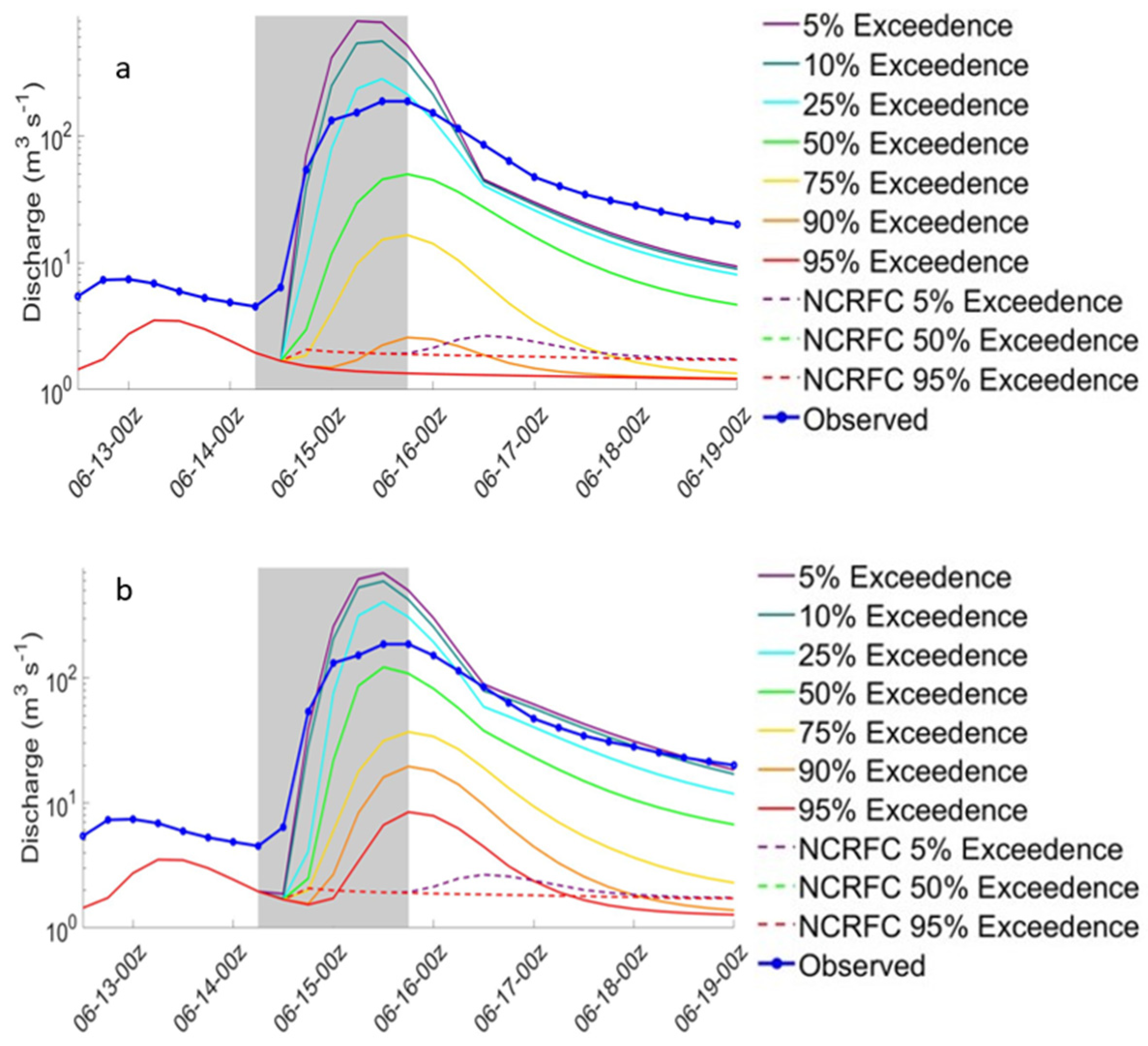
To evaluate the performance of the forecasting technique, error (the difference between the forecasted and observed values), percent difference (PD), and the rank probability score (RPS) were computed. The PD is the average difference between the observed peak discharge (Qobs) and the forecasted peak discharge (Qfcst) divided by the observed peak discharge for a set of N forecasts:
PD = 1 N n = 1 N Q obs , n Q fcst , n Q obs , n × 100 % .
PD was calculated for each probability of exceedance value and averaged by event and basin.
RPS provides an overall measure error for a set (M) of multi-category probabilistic forecasts [46,47,48,49] and is calculated as:
  RPS ¯ = 1 M 1   j = 1 J ( F j O j ) 2
where J is the number of forecast categories, F is the cumulative distribution of the forecast probability across the forecast categories, and O is the cumulative distribution of the probability of the observed event across the forecast categories where the value is either 0 (not observed) or 1 (observed).
The following four flow categories were used based on discharge thresholds defined by the NCRFC for each basin (as in [29]): (1) flood event, defined as the peak discharge exceeding the minor flood discharge; (2) action stage, defined as the peak discharge exceeding the action stage discharge but lower than the minor flood discharge; (3) 50% of the action stage, defined as a the peak discharge greater than half of the action stage but less than the action stage; and (4) nonevent, defined as the peak discharge occurring at less than 50% of the action stage. When comparing NCRFC, HRRRE, and HREF, forecast probabilities for each flow category were calculated using the discharge associated with the 5%, 50%, and 95% exceedance probabilities, as these are the exceedance probabilities used by the NCRFC. A linear interpolation was used to find the forecast probability for the four discharge thresholds. RPS values range from 0 to 1, with 0 indicating a perfect forecast.
To compare the skill of the forecasts created in this study using HRRRE and HREF PQPFs to those issued operationally, RPSs and relative percentage frequency were also computed for probabilistic discharge forecasts generated by the NCRFC. Relative percentage frequency is the frequency of occurrence for a given probability of exceedance. For example, for a reliable forecasting technique, out of 100 rainfall events, it would be expected that the observed rainfall would exceed the 25% probability of exceedance approximately 25 times, while for the 90% probability of exceedance, this would occur approximately 90 times. The NCRFC generates its probability of discharge exceedance forecasts using a 46-member ensemble produced by the Weather Prediction Center (WPC). This ensemble includes members from the Short-Range Ensemble Forecast (SREF) system (both ARW and NMMB), GEFS (Global Ensemble Forecast System), and ECMWF (European Center for Medium-Range Weather Forecasts) ensembles, and the deterministic runs of the GFS, NAM, WRF Hi-res ARW, WRF Hi-Res NMMB, and ECMWF models [50]. The forecasts also take into account WPC’s own QPF forecast and the non-time lagged HREF members. WPC creates rainfall forecasts at 9z and 21z, while the NCRFC generates the probability discharge forecasts at 18z out to 168 h. Thus, NCRFC uses the 9z rainfall forecasts from WPC to make the probability streamflow forecasts. In total, 79 forecasts out of the 109 forecasts generated from the HRRRE and HREF forecasts across seven shared basins were used to compare the NCRFC forecasts to those generated with our PQPF technique.
Although a purely apples-to-apples comparison of our forecasts to operational forecasts was not possible because the forecasts were made at different times, to have the most appropriate comparison possible, the NCRFC probability forecasts closest in time to the HRRRE and HREF run times were used. For example, if 00 UTC HRRRE or HREF output was used, the 18 UTC NCRFC probability forecast generated six hours beforehand was selected, and this occurred on 23 occasions. If 12 UTC HRRRE or HREF output were used, archived radar imagery from the University Corporation for Atmospheric Research [51] was examined to see if any significant rainfall occurred during the 12–18 UTC period. If there was no rainfall in the basin during this period, the NCRFC probability forecasts generated at 18 UTC (six hours after the HRRRE and HREF initializations) were selected, which happened in 41 of the HRRRE and HREF events initialized at 12 UTC. If rainfall was present in the basin before 18 UTC, the previous 18 UTC forecast (18 h prior) was used, which happened 15 times. Thus, this approach resulted in selecting NCRFC forecasts issued before the HRRRE and HREF forecasts almost half the time, with those forecasts issued after the HRRRE and HREF the other half of the time, so any error related to longer lead times for one forecast versus another should be relatively small. Additional factors may influence differences in forecast skill such as the NCRFC forecasts using the much larger WPC forecast ensemble of 46 members compared to HRRRE’s 9 and HREF’s 8 members. In the results that follow, discharge forecasts based on the different probability of exceedance values derived from HRRRE and HREF PQPF or issued by the NCRFC will be identified using the abbreviation of HRRRE/HREF/NCRFC-__% where the percentage value refers to the exceedance value.

3. Results

A comparison of the discharges predicted by the different exceedance probabilities with observed discharges averaged over the full sample of events can be seen in Table 3. As would be expected, the percent differences were positive for the low probability of exceedance forecasts and became negative for the high probability forecasts. Since the switch from positive to negative percent differences happened between the 75% and 90% probability values, and not closer to 50% as might be expected, a positive error in the streamflow forecasts is suggested. Both ensembles produced basin-average rainfall amounts that exceed 225 mm for the 5% exceedance probability forecast. These values are greater than the record 24-h maximum rainfall totals for most places in this region, and thus, they are especially unrealistic as basin averages. The rainfall amounts and percent differences in the discharge forecasts were higher for HREF-based forecasts than for HRRRE-based forecasts. Rainfall inputs from the HRRRE and HREF were more similar for high and low exceedances probabilities than the values in the middle (the biggest differences were at the 25% probability value), resulting in similar percent differences in the discharge forecasts (Table 3). For the low rainfall amounts associated with a high probability of exceedances, a large portion of that rain would go into soil storage in the SAC-SMA model, limiting the amount of water available to produce discharge. At the low exceedance values, the extremely high amounts of rainfall (in both precipitation forecasts) would result in much of the rainfall going to runoff and producing similar high discharges in the SAC-SMA, despite some differences in the basin-average precipitation inputs.
HRRRE-based forecasts had an average RPS of 0.29 (standard deviation, 0.06), which was better than the HREF-based forecasts with an average RPS of 0.36 (standard deviation, 0.09) (Table 4). This difference in RPSs is due to HREF producing higher rainfall amounts compared to HRRRE, which results in forecasts that more seriously over-predict discharge in the higher flow categories. However, when compared to the operational NCRFC forecasts, the HRRRE-based and HREF-based streamflow forecasts had better RPSs; the average RPS for the NCRFC was 0.59 with a standard deviation of 0.07 (Table 4). The poorer RPS for the NCRFC forecasts was due to consistent underprediction of the magnitude of peak discharge for the three different probability values used in these forecasts. Since the NCRFC had a smaller spread in predicted discharge magnitude, the percentage of cases for which the observed discharge remained below that of any of the streamflow forecasts was lower, 60% of events, compared to HRRRE and HREF forecasts, which both were able to capture 100% of the discharge events.
For the HRRRE-based and HREF-based forecasts, RPSs for individual basins ranged from 0.16 to 0.45, except for the Root River at Pilot Mound, MN (RPMM5), which had values of 0.49 and 0.61 (Figure 4). Forecasts for this basin are likely less skillful because RPMM5 is the largest basin studied, resulting in especially large rainfall inputs to the SAC-SMA when the heavy amounts associated with low probabilities of exceedance are applied to all grid points for all time periods. This would make this basin more likely to experience unrealistically large discharges compared to others included in the study and indicates that the PQPF application presented here is likely not suitable to larger watersheds.
The streamflow forecast that most accurately captured the correct relative frequency of the observed peak discharge was HRRRE-95% followed just behind by NCRFC-95% (Figure 5). Forecasts NCRFC-50% and NCRFC-5% greatly underpredicted the frequency of peak discharge amounts, whereas the HREF and HRRRE forecasts overpredicted at those probability levels. Overall, HRRRE did a better job at predicting the frequency of occurrences for the different probability values, having only a slight overprediction in HRRRE-95% and HRRRE-90% that worsened from HRRRE-75% through HRRRE-5%, where there were zero observed occurrences (Figure 5). HREF had poorer results with overprediction, with an observed frequency of exceedance around 77% for HREF-95% and observed frequencies of zero at HREF-25%.
To provide some additional insight into the performance of the streamflow forecasting technique, a flash flood event that occurred in the city of Ames, Iowa, on 14 June 2018 is described in more detail. Ames is located at the junction of the Squaw Creek and Skunk River (Figure 3). On 13 June, both streams were at or below the median discharge of ≈ 4.2 m3 s−1. In the early morning hours (07 UTC) of 14 June, a line of multicellular convection in connection with a cold front moved over the watersheds and produced heavy rain for the next twelve hours. According to the Iowa Mesonet (https://mesonet.agron.iastate.edu/), the system deposited 107 mm of rainfall with a peak rainfall rate of 40.9 mm h−1. Other gauges monitored by the Community Collaborative Rain and Hail Snow Network (COCORAHS) volunteers in the area had total measured accumulations as large as 178 mm. Stage IV data showed that the heaviest total rainfall occurred over the Squaw Creek basin, with the majority of the 6-h accumulation occurring between forecast hours 12 and 18, or 12–18 UTC. The observed peak discharge for the Skunk River was 89.2 m3 s−1 (action stage is 122 m3 s−1), while Squaw Creek’s peak discharge was 120 m3 s−1 (action stage is 108 m3 s−1).
HRRRE and HREF output from the runs at 00 UTC 14 June was used to forecast the discharge for this event. Both the HRRRE and HREF PQPF values suggested that rainfall was going to occur in the region of the Skunk and Squaw basins (Figure 6). HRRRE’s probability forecasts had a northward shift compared to the observed STAGE IV precipitation, while HREF’s forecasts correctly focused the heaviest rain over the basins.
For the Skunk River, the HRRRE and HREF-based forecasts produced hydrographs that were similar to the observed in both in shape and timing (Figure 7). Note that an additional run of the SAC-SMA was completed using STAGE IV measured precipitation data to indicate how the forecast model would perform with QPE. The probability of exceedance value associated with a discharge most similar to the observed discharge was 50%, which resulted in a peak slightly lower than the observed peak discharge (Table 5). The NCRFC forecast largely underpredicted the event on the Skunk River; the discharge associated with only a 5% probability of exceedance was small, at 6.4 m3 s−1, which was almost 14 times smaller than that observed (Table 6).
The forecasted hydrographs for the Squaw Creek were similar to the observed in terms of shape and timing (Figure 8). HRRRE-25% and HREF-50% were the discharge forecasts closest to the observed peak for the two precipitation forecasts tested (Table 5). The NCRFC-5% exceedance discharge forecast was again small: only 10.3 m3 s−1 (Table 6). Although overall, the forecasts overpredicted peak discharge in this example case, the use of ensemble PQPF to generate discharge forecasts associated with a flash flood before rainfall began would have provided a more skillful forecast than what was available from the NCRFC approach.
Given that the frequencies of the observed discharges were poorly matched to the forecast exceedance probabilities, post-processing of the forecasts would likely be one way to improve them. As one preliminary test, a simple calibration was performed iteratively removing a fraction of the forecasted discharge from the discharge predicted at each exceedance probability threshold until the forecasted probabilities of exceedance agreed with the observed frequency of discharge. All 109 cases were used to determine the appropriate average adjustment for each exceedance probability discharge. The size of the reduction in water amount varied greatly between probabilities of exceedance levels and the ensemble being considered. In many cases, more than 50% of the water had to be removed. Using this adjustment, the average RPS for the calibrated HREF-based forecasts improved by 0.1, while HRRRE-based scores improved by a smaller amount of 0.02. Another way to calibrate such forecasts would be to adjust the probability of exceedance so that it matched the observed frequency. Using just the 79 events for which the forecasts had been compared to observed frequencies in Figure 5, a test was performed to determine the impact on the RPSs when the exceedance probabilities were adjusted to match the observed frequencies. This adjustment substantially lowered the discharges associated with the 5% and 50% exceedances, with less adjustment needed for the 95% value. With this test applied to all 109 cases, the average RPS of the adjusted HREF-based forecasts improved by 0.14, which was a nearly 50% improvement, while HRRRE-based scores improved by over 20%, which was a decrease of 0.05. Our sample of cases was not large enough to allow us to split it into a true training set and a separate test set for both of the calibration tests, although the second test did include 30 events independent of those used to adjust the exceedance probabilities.
Techniques such as the Schaake Shuffle [52], which reorders the ensemble output to recover variability in the forcing variables, thereby eliminating the uniform precipitation forcing in time and space, might also lead to improvement. A limiting factor in completing this technique is that it requires the user to have a sizeable sample of historical data to force into the correct order based on climatology. Another post-processing technique to reduce errors in probabilistic streamflow forecasts is the “logistic regression” discussed in [53]. Crochemore et al. [54] showed that bias correcting the precipitation forecasts prior to input into the hydrologic model can lead to improved streamflow forecast skill as measured with the continuous ranked probability skill score. However, they also state that improving the reliability of precipitation forecasts does not always improve the reliability of the streamflow forecasts, and watersheds that had the most “room for improvement” benefitted the most from the bias correction [54]. The testing of more complex pre- and post-processing methods was beyond the scope of the present work but should be examined in future research.

4. Discussion

This study examined a technique that derived rainfall time series for different probabilities of exceedance from ensemble PQPF and used it as input to the SAC-SMA hydrologic model to generate ensemble streamflow forecasts. Two different convection-allowing ensembles, HRRRE and HREF, were tested for 109 events across 11 small-scale basins throughout the Upper Midwest. A variety of different techniques were used to analyze forecasts of peak discharge, and comparisons were made with probabilistic streamflow forecasts generated by the NCRFC.
The HRRRE-based forecasts had the best ability to predict streamflow as indicated by the lowest average RPS of 0.32, and the best agreement between the predicted exceedance probabilities and the frequency that observed discharges exceeded these values. HRRRE likely performed better than HREF because it had lower predicted precipitation amounts for all of the probability of exceedance values examined, which were more similar to the observed rainfall. For HREF-based forecasts, the higher predicted precipitation amounts led to discharge forecasts that, on average, overpredicted the peak discharge. Finally, the NCRFC forecasts frequently underpredicted observed discharge, resulting in the worst RPSs and an increase in the number of times the observed discharges exceeded forecasted discharges associated with the exceedance probabilities. A case study focused on the 14 June Ames flood event suggests that the forecasting technique presented here may provide improved information compared to current forecasting methods to give emergency personnel and the public early information about the possibility of streamflow rises.
The discharge values associated with low probability of exceedance forecasts for both the HRRRE- and HREF-based forecasts were unreasonably large, with no observations having discharges as high as those predicted. The high rainfall amounts associated with low probabilities of exceedance are applied at all grid points within a basin, resulting in unreasonably high discharge forecasts. This problem was especially prevalent for the Root River, the largest basin examined, indicating that the overprediction worsens with basin size, as would be expected due to the application of the same exceedance amounts at all grid points in a basin.
This problem could be reduced in the future by calibrating the probability of exceedance values, such as by adjusting them to match observed frequencies during a training period, or by decreasing rainfall amounts associated with given probabilities of exceedance so that the magnitude of the predicted discharges would be reduced, or by calibration of the streamflow forecasts related to the exceedance values themselves. Two simple preliminary tests applied to the streamflow forecasts resulted in improvements in skill for the HREF-based forecast, with smaller improvements for the HRRRE-based one. Another refinement that might improve this technique would be to use an analysis of the spatial distribution of QPE from multiple warm-season rainfall events to determine the typical areal pattern of precipitation. This analysis of the spatial distribution would require the ability to distinguish between different types of convective systems occurring in the model output. Then, the distribution pattern could be used to adjust the rainfall amounts associated with PQPF values over the basins. Combining these techniques would allow the use of multiple different exceedance values in the spatial averaging, instead of a single blanket exceedance probability. This would allow more accurate precipitation forcing to be fed into the hydrologic model during each timestep and take advantage of the presumed value added by the analysis that enters into the PQPF that is absent from the raw QPF members.

Author Contributions

Conceptualization, K.F. and W.G.; methodology, A.R.G., K.J.F., and W.A.G.J.; software, A.R.G. and W.A.G.J.; validation, A.R.G., K.J.F., and W.A.G.J.; formal analysis, A.R.G.; investigation, A.R.G.; resources, A.R.G., K.J.F., W.A.G.J. and B.R.; data curation, A.R.G. and B.R.; writing—original draft preparation, A.R.G.; writing—review and editing, A.R.G., K.J.F., W.A.G.J. and B.R.; supervision, K.J.F. and W.A.G.J.; project administration, K.J.F. and W.A.G.J.; funding acquisition, K.J.F. and W.A.G.J. All authors have read and agreed to the published version of the manuscript.

Funding

This work was funded by NOAA CSTAR Award NA17NWS4680005.

Acknowledgments

The author would like to thank the North Central River Forecast Center, especially Brian Connelly, for providing the initial conditions data for the SAC-SMA model and the probability forecasts from the NCRFC.

Conflicts of Interest

The authors declare no conflict of interest.

References

  1. Nguyen, P.; Thorstensen, A.; Sorooshian, S.; Hsu, K.; Aghakouchak, A. Flood forecasting and inundation mapping using HiResFlood-UCI and near-real-time satellite precipitation data: The 2008 Iowa flood. J. Hydrometeorol. 2015, 16, 1171–1183. [Google Scholar] [CrossRef]
  2. Krajewski, W.F.; Ceynar, D.; Demir, I.; GosKa, R.; Kruger, A.; Langel, C.; Mantilla, R.; Niemeier, J.; Quintero, F.; Seo, B.-C.; et al. Real-time flood forecasting and information system for the state of Iowa. Bull. Am. Meteorol. Soc. 2017, 98, 539–554. [Google Scholar] [CrossRef]
  3. Cuo, L.; Pagano, T.C.; Wang, Q.J. A Review of Quantitative Precipitation Forecasts and Their Use in Short- to Medium-Range Streamflow Forecasting. J. Hydrometeorol. 2011, 12, 713–728. [Google Scholar] [CrossRef]
  4. Seo, B.C.; Quintero, F.; Krajewski, W.F. High-resolution QPF uncertainty and its implications for flood prediction: A case study for the eastern Iowa flood of 2016. J. Hydrometeorol. 2018, 19, 1289–1304. [Google Scholar] [CrossRef]
  5. Davolio, S.; Miglietta, M.M.; Diomede, T.; Marsigli, C.; Morgillo, A.; Moscatello, A. A meteo-hydrological prediction system based on a multi-model approach for precipitation forecasting. Nat. Hazards Earth Syst. Sci. 2008, 8, 143–159. [Google Scholar] [CrossRef]
  6. Wu, J.; Lu, G.; Wu, Z. Flood forecasts based on multi-model ensemble precipitation forecasting using a coupled atmospheric-hydrological modeling system. Nat. Hazards 2014, 74, 325–340. [Google Scholar] [CrossRef]
  7. Fritsch, J.M.; Carbone, R.E. Improving Quantitative Precipitation Forecasts in the Warm Season: A USWRP Research and Development Strategy. Bull. Am. Meteorol. Soc. 2004, 85, 955–966. [Google Scholar] [CrossRef] [Green Version]
  8. Gallus, W.A. Rainfall Forecasting. The Challenge of Warm-Season Convective Precipitation Forecasting. In Hydrological Science and Engineering; Wong, T.S.W., Ed.; Nova Science Publishers: Hauppauge, NY, USA, 2012; pp. 129–160. ISBN 978-61942-134-9. [Google Scholar]
  9. Moser, B.A.; Gallus, W.A.; Mantilla, R. An initial assessment of radar data assimilation on warm season rainfall forecasts for use in hydrologic models. Weather Forecast. 2015, 30, 1491–1520. [Google Scholar] [CrossRef]
  10. Ebert, E.E.; Damrath, U.; Wergen, W.; Baldwin, M.E. The WGNE Assessment of Short-term Quantitative Precipitation Forecasts. Bull. Am. Meteorol. Soc. 2003, 84, 481–492. [Google Scholar] [CrossRef]
  11. Cluckie, I.D.; Xuan, Y.; Wang, Y. Uncertainty analysis of hydrological ensemble forecasts in a distributed model utilising short-range rainfall prediction. Hydrol. Earth Syst. Sci. 2009, 13, 293–303. [Google Scholar] [CrossRef] [Green Version]
  12. Nielsen, E.R.; Schumacher, R.S. Using Convection-Allowing Ensembles to Understand the Predictability of an Extreme Rainfall Event. Mon. Weather Rev. 2016, 144, 3651–3676. [Google Scholar] [CrossRef]
  13. Duda, J.D.; Gallus, W.A. The impact of large-scale forcing on skill of simulated convective initiation and upscale evolution with convection-allowing grid spacings in the WRF. Weather Forecast. 2013, 28, 994–1018. [Google Scholar] [CrossRef] [Green Version]
  14. Golding, B.W. Quantitative precipitation forecasting in the UK. J. Hydrol. 2000, 239, 286–305. [Google Scholar] [CrossRef]
  15. Eckel, F.A.; Mass, C.F. Aspects of Effective Mesoscale, Short-Range Ensemble Forecasting. Weather Forecast. 2005, 20, 328–350. [Google Scholar] [CrossRef]
  16. Cintineo, R.; Otkin, J.A.; Xue, M.; Kong, F. Evaluating the Performance of Planetary Boundary Layer and Cloud Microphysical Parameterization Schemes in Convection-Permitting Ensemble Forecasts Using Synthetic GOES-13 Satellite Observations. Mon. Weather Rev. 2014, 142, 163–182. [Google Scholar] [CrossRef] [Green Version]
  17. Banks, R.F.; Tiana-Alsina, J.; Baldasano, J.M.; Rocadenbosch, F.; Papayannis, A.; Solomos, S.; Tzanis, C.G. Sensitivity of boundary-layer variables to PBL schemes in the WRF model based on surface meteorological observations, lidar, and radiosondes during the HygrA-CD campaign. Atmos. Res. 2016, 176–177, 185–201. [Google Scholar] [CrossRef]
  18. Cloke, H.L.; Pappenberger, F. Ensemble flood forecasting: A review. J. Hydrol. 2009, 375, 613–626. [Google Scholar] [CrossRef]
  19. Dowell, D.; Alexander, C.; Alcott, T.; Ladwig, T. HRRR Ensemble (HRRRE) Guidance 2018 HWT Spring Experiment. Available online: https://rapidrefresh.noaa.gov/internal/pdfs/2018_Spring_Experiment_HRRRE_Documentation.pdf (accessed on 1 June 2018).
  20. Avolio, E.; Federico, S.; Miglietta, M.M.; Lo Feudo, T.; Calidonna, C.R.; Sempreviva, A.M. Sensitivity analysis of WRF model PBL schemes in simulating boundary-layer variables in southern Italy: An experimental campaign. Atmos. Res. 2017, 192, 58–71. [Google Scholar] [CrossRef]
  21. Roberts, B.; Jirak, I.L.; Clark, A.J.; Weiss, S.J.; Kain, J.S. PostProcessing and Visualization Techniques for Convection-Allowing Ensembles. Bull. Am. Meteorol. Soc. 2019, 100, 1245–1258. [Google Scholar] [CrossRef] [Green Version]
  22. Clark, A.J. Generation of Ensemble Mean Precipitation Forecasts from Convection-Allowing Ensembles. Weather Forecast. 2017, 32, 1569–1583. [Google Scholar] [CrossRef]
  23. Leith, C.E. Theoretical Skill of Monte Carlo Forecasts. Mon. Weather Rev. 1974, 102, 409–418. [Google Scholar] [CrossRef] [Green Version]
  24. Buizza, R.; Miller, M.; Palmer, T.N. Stochastic representation of model uncertainties in the ECMWF ensemble prediction system. Q. J. R. Meteorol. Soc. 1999, 460, 2887–2908. [Google Scholar] [CrossRef]
  25. Werner, K.; Brandon, D.; Clark, M.; Gangopadhyay, S. Incorporating medium-range numerical weather model output into the Ensemble Streamflow Prediction system of the National Weather Service. J. Hydrometeorol. 2005, 6, 101–114. [Google Scholar] [CrossRef] [Green Version]
  26. Ebert, E.E. Ability of a poor man’s ensemble to predict the probability and distribution of precipitation. Mon. Weather Rev. 2001, 129, 2461–2480. [Google Scholar] [CrossRef]
  27. Ferraris, L.; Rudari, R.; Siccardi, F. The Uncertainty in the Prediction of Flash Floods in the Northern Mediterranean Environment. J. Hydrometeorol. 2002, 3, 714–727. [Google Scholar] [CrossRef]
  28. Yan, H.; Gallus, W.A., Jr. An Evaluation of QPF from the WRF, NAM, and GFS Models Using Multiple Verification Methods over a Small Domain. Weather Forecast. 2016, 31, 1363–1379. [Google Scholar] [CrossRef]
  29. Carlberg, B.; Franz, K.; Gallus, W., Jr. Submitted, A method to account for QPF spatial displacement errors in short-term ensemble streamflow forecasting. Water 2020. [Google Scholar]
  30. Reed, S.M.; MacFarlane, A. Validation of NWS Hydrologic Ensemble Forecast Service (HEFS) Real-time Products at the Middle Atlantic River Forecast Center. In Proceedings of the 34th Conference on Hydrology, Boston, MA, USA, 12–16 January 2020; American Meteorological Society: Boston, MA, USA, 2020. [Google Scholar]
  31. Stensrud, D.J.; Yussouf, N. Reliable Probabilistic Quantitative Precipitation Forecasts from a Short-Range Ensemble Forecasting System. Weather Forecast. 2007, 22, 3–17. [Google Scholar] [CrossRef]
  32. Jeanne-Rose, R.; Madsen, H.; Ole, M. A Methodology for Probabilistic Real-Time Forecasting—An Urban Case Study. J. Hydroinform. 2013, 15, 751–762. [Google Scholar] [CrossRef] [Green Version]
  33. Thompson, G.; Eidhammer, T. A Study of Aerosol Impacts on Clouds and Precipitation Development in a Large Winter Cyclone. J. Atmos. Sci. 2014, 71, 3636–3658. [Google Scholar] [CrossRef]
  34. Nakanishi, M.; Niino, H. Development of an improved turbulence closure model for the atmospheric boundary layer. J. Meteorol. Soc. Jpn. 2009, 87, 895–912. [Google Scholar] [CrossRef] [Green Version]
  35. Skamarock, W.C.; Klemp, J.B.; Dudhia, J.; Gill, D.O.; Barker, D.; Duda, M.G.; Powers, J.G. A Description of the Advanced Research WRF Version 3; Citeseer: Boulder, CO, USA, 2008. [Google Scholar]
  36. Janjic, Z.; Gall, R. Scientific Documentation of the NCEP Nonhydrostatic Multiscale Model on the B Grid (NMMB). Prt 1 Dynamics; Citeseer: Boulder, CO, USA, 2012. [Google Scholar]
  37. Environmental Modeling Center, N.W.S. NAM 2017. Available online: https://www.emc.ncep.noaa.gov/NAM/mconf.php (accessed on 1 October 2018).
  38. Janjić, Z.I. The Step-Mountain Eta Coordinate Model: Further Developments of the Convection, Viscous Sublayer, and Turbulence Closure Schemes. Mon. Weather Rev. 1994, 122, 927–945. [Google Scholar] [CrossRef] [Green Version]
  39. Hong, S.; Lim, J. The WRF single-moment 6-class microphysics scheme (WSM6). J. Korean Meteorol. Soc. 2006, 42, 129–151. [Google Scholar]
  40. Hong, S.-Y.; Noh, Y.; Dudhia, J. A New Vertical Diffusion Package with an Explicit Treatment of Entrainment Processes. Mon. Weather Rev. 2006, 134, 2318–2341. [Google Scholar] [CrossRef] [Green Version]
  41. Aligo, E.B.; Ferrier, J.; Carley, E.; Rogers, M.; Pyle, S.; Weiss, J.; Jirak, I.L. Modified Microphysics for Use in High-Resolution NAM Forecasts. In Proceedings of the 27th Conference on Severe Storms, Madison, WI, USA, 2–7 November 2014. [Google Scholar]
  42. Azizan, I.; Karin, S.A.B.A.; Raju, S.S.K. Fitting rainfall data by using cubic spline interpolation. In Proceedings of the MATEC Web Conference; EDP Sciences: Paris, France, 2018; Volume 225, p. 9. [Google Scholar]
  43. Lin, Y.; Mitchell, K.E. The NCEP Stage II/IV hourly preciptiation analysis development and applications. In Proceedings of the 19th Conference on Hydrology, 9–13 January 2005; American Meteorological Society: San Diego, CA, USA, 2005. [Google Scholar]
  44. Burnash, R.J.C.; Ferral, L.; McGuire, R.A. A Generalized Streamflow Simulation System: Conceptual Models for Digital Computers; Joint Federal and State River Forecast Center, U.S. National Weather Service, and California Department of Water Resources Techinical Report; California Department of Water Resources: Sacramento, CA, USA, 1973.
  45. Burnash, R.J.C. The NWS River Forecast System-Catchment Modeling. In Computer Models of Watershed Hydrology; Singh, V., Ed.; Water Resources Publication: Lone Tree, CO, USA, 1995; pp. 311–366. [Google Scholar]
  46. Epstein, E.S. A scoring system for probability forecasts of ranked categories. J. Appl. Meteorol. 1969, 8, 985–987. [Google Scholar] [CrossRef] [Green Version]
  47. Wilks, D.S. Forecast verification. In Statistical Methods in the Atmospheric Sciences; Academic Press: Boston, MA, USA, 1995; pp. 233–283. ISBN 978-0-12-385022-5. [Google Scholar]
  48. Murphy, A.H. On the “Ranked Probability Score”. J. Appl. Meteorol. 1969, 8, 988–989. [Google Scholar] [CrossRef] [Green Version]
  49. Murphy, A.H. A Note on the Ranked Probability Score. J. Appl. Meteorol. 1971, 10, 155–156. [Google Scholar] [CrossRef] [Green Version]
  50. NWS about WPC’s PQPF and Percentile QPF Products. Available online: https://www.wpc.ncep.noaa.gov/pqpf/about_pqpf_products.shtml (accessed on 8 April 2019).
  51. UCAR Image Archive—Meteorological Case Study Selection Kit. Available online: http://www2.mmm.ucar.edu/imagearchive/ (accessed on 1 November 2018).
  52. Clark, M.; Gangopadhyay, S.; Hay, L.; Rajagopalan, B.; Wilby, R. The Schaake Shuffle: A Method for Reconstructing Space—Time Variability in Forecasted Precipitation and Temperature Fields. J. Hydrometeorol. 2004, 5, 243–262. [Google Scholar] [CrossRef] [Green Version]
  53. Roulin, E.; Vannitsem, S. Postprocessing of Ensemble Precipitation Predictions with Extended Logistic Regression Based on Hindcasts. Mon. Weather Rev. 2012, 140, 874–888. [Google Scholar] [CrossRef]
  54. Crochemore, L.; Ramos, M.-H.; Papenberger, F. Bias correcting precipitation forecasts to improve the skill of seasonal streamflow forecasts. Hydrol. Earth Syst. Sci. 2016, 20, 3601–3618. [Google Scholar] [CrossRef] [Green Version]
Publisher’s Note: MDPI stays neutral with regard to jurisdictional claims in published maps and institutional affiliations.
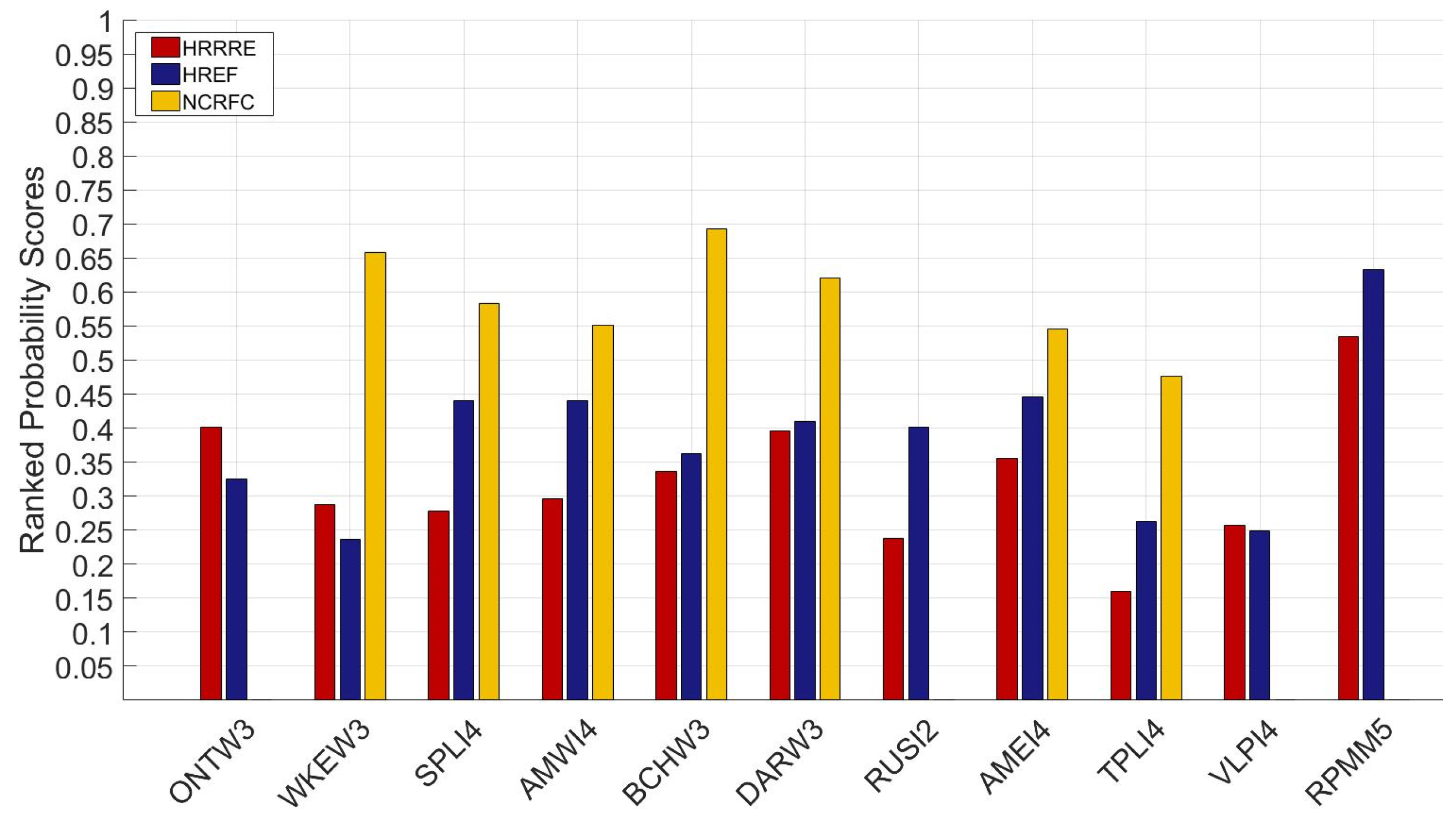
Figure 1. Location of the study basins.
Water 12 02860 g001
Figure 2. Example of the data interpolation technique used to transform the Probabilistic Quantitative Precipitation Forecast (PQPF) values from the ensembles into rainfall amounts for various probabilities of exceedance, with (a) showing the PQPF values from the High-Resolution Rapid Refresh Ensemble (HRRRE, blue circles) with the additional boundary values (green triangles) from zero rainfall and the absolute highest member rainfall amount inside the research domain, and (b) showing rainfall amounts associated with the probability of exceedance values (red diamonds) used in the study, after running the Piecewise Cubic Hermite Interpolating Polynomial (PCHIP) interpolation program.
Water 12 02860 g002
Figure 3. An example of clipping the HRRRE’s probability values for rainfall exceeding 25.4 mm over the Skunk River on 14 June from 06-12 UTC.
Water 12 02860 g003
Figure 4. RPS for the eleven basins (labeled using NCRFC abbreviations) arranged in order from the smallest (left) to the largest (right) in area.
Water 12 02860 g004
Figure 5. Relative frequency of observations exceeding the forecasts for different forecast probability of exceedance values. All datasets use the same 79 events that are common between the NCRFC and PQPF datasets.
Water 12 02860 g005
Figure 6. PQPF for the period 12–18 UTC on 14 June from the HRRRE (ac) and HREF (eg) initialized at 00 UTC 14 June, and Stage IV rainfall accumulations (12–18 UTC in d, 00 UTC 14 June–12 UTC 15 June in g) over the central Iowa area. The black outlines represent the basins of the Skunk River (right) and Squaw Creek (left). The six panels on the left show PQPF at three different thresholds (left 12.7 mm, middle 25.4 mm, and right 50.8 mm). The dashed red line represents the Stage IV accumulation exceeding that rainfall threshold.
Water 12 02860 g006
Figure 7. Hydrographs from all exceedance levels in the (a) HRRRE-based and (b) HREF-based forecasts for the 14 June 2018 event for Skunk River, with the NCRFC forecasts shown in dashed lines, and the observed discharge from the USGS gauge (solid blue line with closed circles). The gray box in the background signifies the time steps where PQPF was used. The y-axis displays the forecasted and observed discharges in a logarithmic scale, while the x-axis shows the date and time.
Water 12 02860 g007
Figure 8. Same as in Figure 7, except for the Squaw Creek.
Water 12 02860 g008
Table 1. Study basins, basin area, United States Geological Survey (USGS) gauge number, National Weather Service (NWS) forecast point identification, and the number of events analyzed for each basin. Bold signifies the gauges for which the North Central River Forecasts Center (NCRFC) issues probabilistic streamflow forecasts.
BasinAreaUSGS Gauge StationNWS IDNumber of Events
Kickapoo at Ontario (WI)303 km205407470ONTW310
Fox River at Waukesha (WI)326 km205543830WKEW311
Turkey River at Spillville (IA)458 km205411600SPLI411
Squaw Creek at Ames (IA)528 km205470500AMEI414
Pecatonica East at Blanchardville (WI)572 km205433000BCHW314
Pecatonica West at Darlington (WI)707 km205432500DARW38
Des Plains at Russell (IL)785 km205527800RUSI26
South Skunk River at Ames (IA)816 km205470000AMWI414
Wapsipinicon River at Tripoli (IA)896 km205420680TLPI47
Volga River at Littleport (IA)901 km205412400VLPI46
Root River at Pilot Mound (MN)1463 km205383950PRMM58
Table 2. Member configurations for the High-Resolution Ensemble Forecast version 2.0 (HREF) and High-Resolution Rapid Refresh Ensemble (HRRRE) ensembles during the study period, including initial conditions (ICs), lateral boundary conditions (LBCs), microphysics, and planetary boundary layer schemes (PBL), grid spacing, and the number of vertical levels.
MemberICs/LBCsMicrophysicsPBLGrid SpacingVert. Levels
HREF HRW NSSL NAM/NAM WSM6MYJ3.2 km40
HREF HRW ARW RAP/GFS WSM6YSU3.2 km50
HREF HRW MMB RAP/GFS Ferrier-AligoMYJ3.2 km50
HREF NAM CONUS NEST NAM/NAMFerrier-AligoMYJ3 km60
HRRRE
9-MEMBERS
GDAS
(with random permutations added)
Thompson aerosol-awareMYNN3 km51
Table 3. Average error in   m 3   s 1 and percent difference (PD) for the probabilistic streamflow predictions and basin-averaged rainfall amounts for 36 h forecasts in mm for all 11 basins and 109 events studied for each probability of exceedance.
Probability of Exceedance5%10%25%50%75%90%95%
ErrorHRRRE-based81856628395.79.46−20.9−28.1
HREF-based81066642219153.5−2.83−17.3
PDHRRRE-based3330%2150%1000%321%47.6%−26.5%−43.5%
HREF-based3470%2720%1500%619%175%15.8%−20.7%
Averaged RainfallHRRRE22617611973.940.121.814.0
HREF24921515910361.234.823.1
Table 4. Averages and standard deviations for rank probability scores (RPSs) for HRRRE, HREF, and NCRFC ensemble streamflow predictions for the seven shared (all 11) basins.
Average RPSStandard Deviation RPS
HRRRE-based0.29 (0.28)0.06 (0.10)
HREF-based0.36 (0.34)0.09 (0.12)
NCRFC0.590.07
Table 5. Error (m3 s−1) for Skunk River and Squaw Creek ensemble streamflow predictions for different probability of exceedance values for the 14 June event.
95%90%75%50%25%10%5%
Skunk RiverHRRRE-based−185−185−171−13794.3371615
HREF-based−179−167−150−64.6220411507
Squaw CreekHRRRE-based−86.7−85.2−66.0−19.5157402620
HREF-based−86.4−77.9−54.7−9.60163430561
Table 6. Percent of discharge that needed to be removed from the forecasted probabilities of exceedance to calibrate them so that the observed frequency of discharge agreed with the probability of exceedance values for the HRRRE-based and HREF-based probabilistic streamflow forecasts.
Probability of Exceedance5%10%25%50%75%90%95%
HRRRE-based60%65%64%62%45%28%22%
HREF-based74%80%79%79%72%54%48%

