Phytoplankton–Macrophyte Interaction in the Lagoon of Venice (Northern Adriatic Sea, Italy)


Abstract
1. Introduction
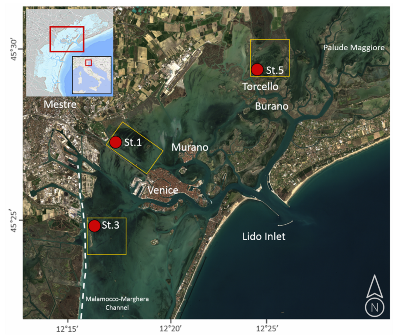
2. Area of Studies
3. Materials and Methods
3.1. Hydrochemical Parameters
3.2. Statistical Analyses
3.3. Satellite Data and Processing
4. Results
4.1. Hydrochemical Data: Comparison of Stations
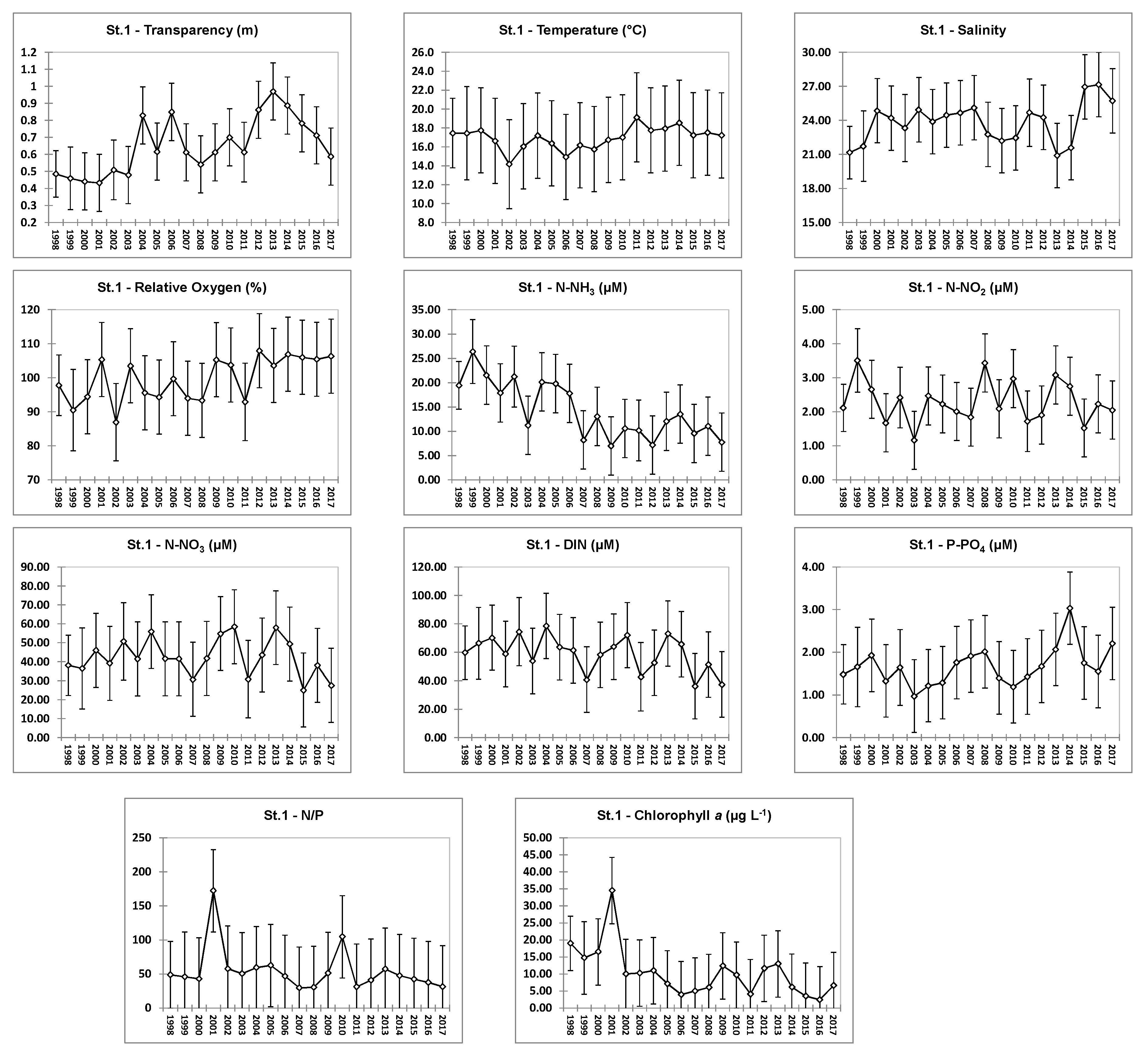
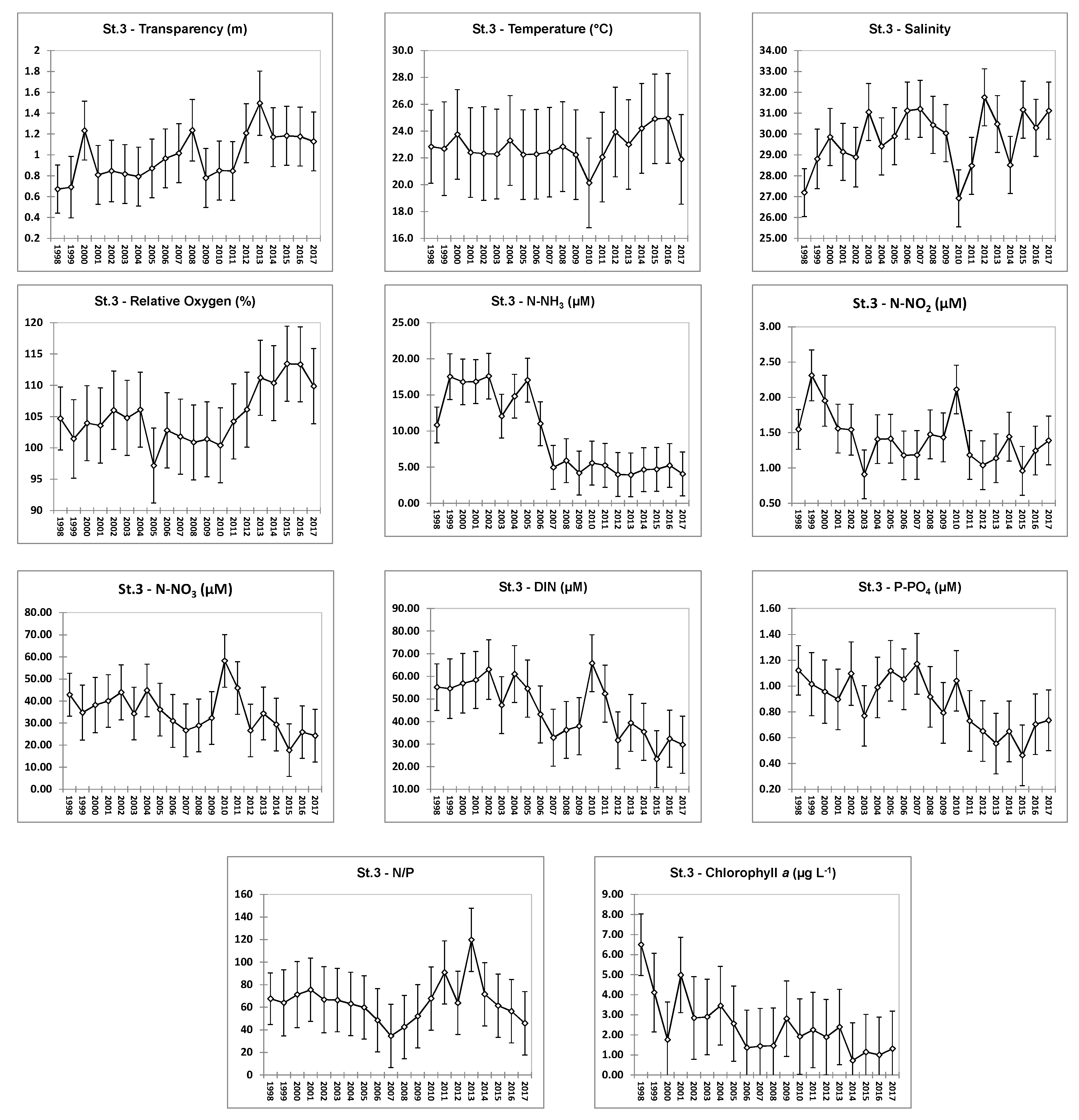
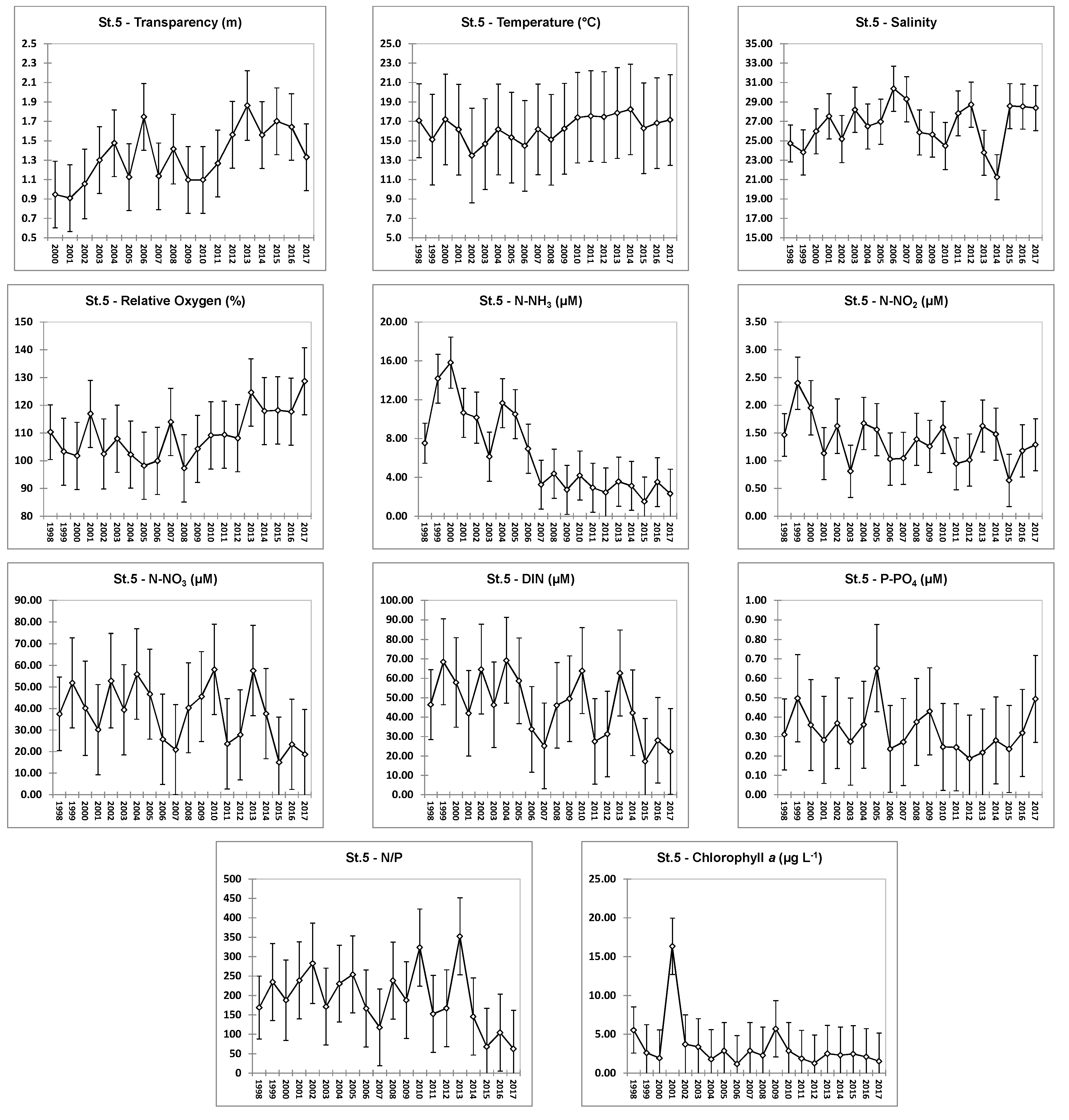
4.2. Hydrochemical Data: Interannual Variability
4.3. Macrophyte Coverage
4.4. Statistical Analysis of Trends
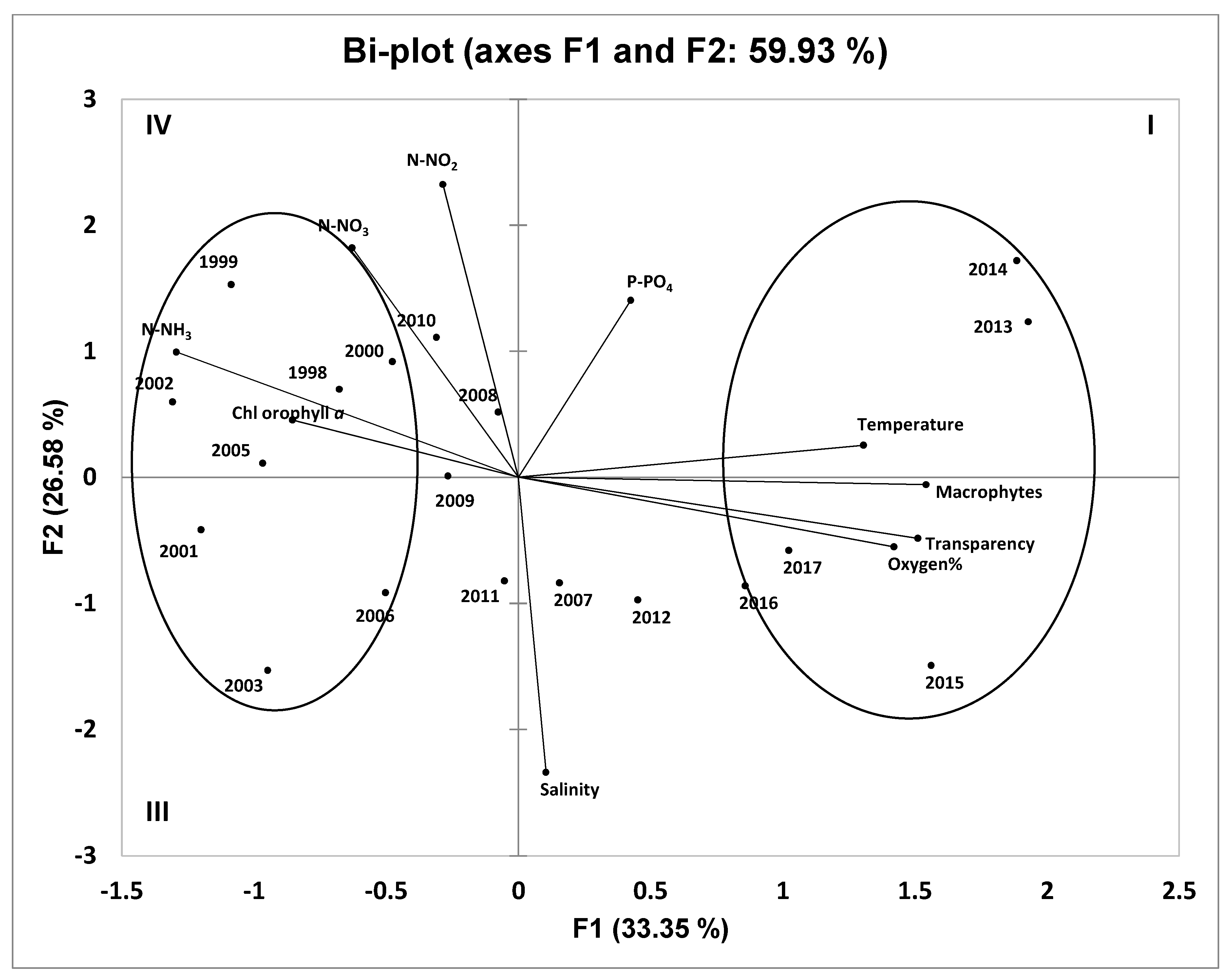
4.5. Principal Component Analysis of Hydrochemical Parameters and Macrophyte Coverage
5. Discussion
Supplementary Materials
Author Contributions
Funding
Acknowledgments
Conflicts of Interest
References
- Barnes, R.S.K. Coastal Lagoons, 1st ed.; Cambridge University Press: Cambridge, UK, 1980; p. 106. ISBN 780521234221. [Google Scholar]
- Pérez-Ruzafa, A.; Marcos, C.; Perez-Ruzafa, I.M.; Pérez-Marcos, M. Coastal lagoons: “Transitional ecosystems” between transitional and coastal waters. J. Coast. Conserv. 2010, 15, 369–392. [Google Scholar] [CrossRef]
- Newton, A.; Icely, J.; Cristina, S.C.V.; Brito, A.C.; Cardoso, A.C.; Colijn, F.; Riva, S.D.; Gertz, F.; Hansen, J.W.; Holmer, M.; et al. An overview of ecological status, vulnerability and future perspectives of European large shallow, semi-enclosed coastal systems, lagoons and transitional waters. Estuar. Coast. Shelf Sci. 2014, 140, 95–122. [Google Scholar] [CrossRef]
- Orfanidis, S.; Panayotidis, P.; Stamatis, N. An insight to the ecological evaluation index (EEI). Ecol. Indic. 2003, 3, 27–33. [Google Scholar] [CrossRef]
- Giordani, G.; Zaldívar, J.; Viaroli, P. Simple tools for assessing water quality and trophic status in transitional water ecosystems. Ecol. Indic. 2009, 9, 982–991. [Google Scholar] [CrossRef]
- Sfriso, A.; Facca, C.; Bon, D.; Buosi, A. Macrophytes and ecological status assessment in the Po delta transitional systems, Adriatic Sea (Italy). Application of Macrophyte Quality Index (MaQI). Acta Adriat. 2016, 57, 209–225. [Google Scholar]
- McGlathery, K.; Sundbäck, K.; Anderson, I. Eutrophication in shallow coastal bays and lagoons: The role of plants in the coastal filter. Mar. Ecol. Prog. Ser. 2007, 348, 1–18. [Google Scholar] [CrossRef]
- Adriano, S.; Chiara, F.; Antonio, M. Sedimentation rates and erosion processes in the lagoon of Venice. Environ. Int. 2005, 31, 983–992. [Google Scholar] [CrossRef]
- Duarte, C.M. Submerged aquatic vegetation in relation to different nutrient regimes. Ophelia 1995, 41, 87–112. [Google Scholar] [CrossRef]
- Ralph, P.J.; Durako, M.; Enríquez, S.; Collier, C.; Doblin, M. Impact of light limitation on seagrasses. J. Exp. Mar. Biol. Ecol. 2007, 350, 176–193. [Google Scholar] [CrossRef]
- Solidoro, C.; Bandelj, V.; Bernardi, F.A.; Camatti, E.; Ciavatta, S.; Cossarini, G.; Facca, C.; Franzoi, P.; Libralato, S.; Canu, D.M.; et al. Response of Venice Lagoon Ecosystem to Natural and Anthropogenic Pressures over the Last 50 Years. In Coastal Lagoons: Critical Habitats of Environmental Change; Kennish, M.J., Paerl, H.W., Eds.; CRC Press, Taylor and Francis: Boca Raton, FL, USA, 2010; pp. 483–511. [Google Scholar]
- Braga, F.; Scarpa, G.M.; Brando, V.E.; Manfè, G.; Zaggia, L. COVID-19 lockdown measures reveal human impact on water transparency in the Venice Lagoon. Sci. Total. Environ. 2020, 736, 139612. [Google Scholar] [CrossRef]
- Kosten, S.; Jeppesen, E.; Huszar, V.L.M.; Mazzeo, N.; Van Nes, E.H.; Peeters, E.T.; Scheffer, M. Ambiguous climate impacts on competition between submerged macrophytes and phytoplankton in shallow lakes. Freshw. Biol. 2011, 56, 1540–1553. [Google Scholar] [CrossRef]
- Sfriso, A.; Facca, C.; Ghetti, P. Temporal and spatial changes of macroalgae and phytoplankton in a Mediterranean coastal area: The Venice lagoon as a case study. Mar. Environ. Res. 2003, 56, 617–636. [Google Scholar] [CrossRef]
- Sfriso, A.A.; Facca, C.; Ghetti, P.F. Validation of the Macrophyte Quality Index (MaQI) set up to assess the ecological status of Italian marine transitional environments. Hydrobiology 2008, 617, 117–141. [Google Scholar] [CrossRef]
- Facca, C.; Aubry, F.B.; Socal, G.; Ponis, E.; Acri, F.; Bianchi, F.; Giovanardi, F.; Sfriso, A.A. Description of a Multimetric Phytoplankton Index (MPI) for the assessment of transitional waters. Mar. Pollut. Bull. 2014, 79, 145–154. [Google Scholar] [CrossRef] [PubMed]
- Sfriso, A.; Marcomini, A.; Pavoni, B. Relationships between macroalgal biomass and nutrient concentrations in a hypertrophic area of the Venice Lagoon. Mar. Environ. Res. 1987, 22, 297–312. [Google Scholar] [CrossRef]
- CoRiLa. Monitoraggio Matrice Praterie a Fanerogame. Available online: http://ckan.corila.it/dataset/fanerogame (accessed on 20 July 2020).
- Sfriso, A.; Pavoni, B. Macroalgae and phytoplankton competition in the central Venice lagoon. Environ. Technol. 1994, 15, 1–14. [Google Scholar] [CrossRef]
- Curiel, D.; Rismondo, A.; Bellemo, G.; Marzocchi, M. Macroalgal biomass and species variations in the Lagoon of Venice (Northern Adriatic Sea, Italy): 1981–1998. Sci. Mar. 2004, 68, 57–67. [Google Scholar] [CrossRef]
- Sfriso, A.; Marcomini, A. Decline of Ulva growth in the lagoon of Venice. Bioresour. Technol. 1996, 58, 299–307. [Google Scholar] [CrossRef]
- Facca, C. Trophic Conditions in the Waters of the Venice Lagoon (Northern Adriatic Sea, Italy). Open Oceanogr. J. 2011, 5, 1–13. [Google Scholar] [CrossRef][Green Version]
- Facca, C.; Ceoldo, S.; Pellegrino, N.; Sfriso, A.A. Natural Recovery and Planned Intervention in Coastal Wetlands: Venice Lagoon (Northern Adriatic Sea, Italy) as a Case Study. Sci. World J. 2014, 2014, 1–15. [Google Scholar] [CrossRef]
- Rismondo, A.; Curiel, D.; Scarton, F.; Mion, D.; Pierini, A.; Caniglia, G. Distribution of Zostera noltii, Zostera marina and Cymodocea nodosa in Venice lagoon. In Flooding and Environmental Challenges for Venice and its Lagoon: State of Knowledge; Fletcher, C.A., Spencer, T., Eds.; Cambridge University Press: Cambridge, UK, 2005; pp. 567–572. ISBN 9780521840460. [Google Scholar]
- Voltolina, D. The Phytoplankton of The Lagoon of Venice: November 1971—November 1972; Pubblicazioni Stazione Zoologica: Napoli, Italy, 1975; Volume 39, pp. 206–340. [Google Scholar]
- Alberighi, L.; Bianchi, F.; Cioce, F.; Socal, G. Osservazioni durante un bloom di Skeletonema costatum in prossimità della centrale termoelettrica ENEL di Fusina Porto-Marghera (Venezia). Oebalia 1992, 17, 321–322. [Google Scholar]
- Socal, G.; Bianchi, F.; Alberighi, L. Effects of thermal pollution and nutrient discharges on a spring phytoplankton bloom in the industrial area of the Lagoon of Venice. Vie Milieu 1999, 49, 19–31. [Google Scholar]
- Facca, C.; Sfriso, A.; Socal, G. Changes in Abundance and Composition of Phytoplankton and Microphytobenthos due to Increased Sediment Fluxes in the Venice Lagoon, Italy. Estuar. Coast. Shelf Sci. 2002, 54, 773–792. [Google Scholar] [CrossRef]
- Aubry, F.B.; Acri, F.; Bianchi, F.; Pugnetti, A. Looking for patterns in the phytoplankton community of the Mediterranean microtidal Venice Lagoon: Evidence from ten years of observations. Sci. Mar. 2013, 77, 47–60. [Google Scholar] [CrossRef]
- Bianchi, F.; Acri, F.; Alberighi, L.; Bastianini, M.; Boldrin, A.; Cavalloni, B.; Cioce, F.; Comaschi, A.; Rabitti, S.; Socal, G.; et al. Biological variability in the Venice Lagoon. In The Venice Lagoon Ecosystem. Inputs and Interactions between Land and Sea; Lasserre, P., Marzollo, A., Eds.; UNESCO and Parthenon Publishing Press: Paris, France, 2000; pp. 97–126. ISBN 1850700834. [Google Scholar]
- Acri, F.; Braga, F.; Aubry, F.B.B. Long-term dynamics in nutrients, chlorophyll a and water quality parameters in the Lagoon of Venice. Sci. Mar. 2020, 84. [Google Scholar] [CrossRef]
- Sfriso, A.; Buosi, A.; Mistri, M.; Munari, C.; Franzoi, P.; Sfriso, A.A. Long-term changes of the trophic status in transitional ecosystems of the northern Adriatic Sea, key parameters and future expectations: The lagoon of Venice as a study case. Nat. Conserv. 2019, 34, 193–215. [Google Scholar] [CrossRef]
- Malthus, T.J. Bio-optical Modeling and Remote Sensing of Aquatic Macrophytes. In Bio-optical Modeling and Remote Sensing of Inland Waters; Mishra, D.R., Ogashawara, I., Gitelson, A., Eds.; Elsevier: Amsterdam, The Netherlands, 2017; pp. 263–308. [Google Scholar]
- Hedley, J.D.; Roelfsema, C.; Brando, V.E.; Giardino, C.; Kutser, T.; Phinn, S.; Mumby, P.J.; Barrilero, O.; Laporte, J.; Koetz, B. Coral reef applications of Sentinel-2: Coverage, characteristics, bathymetry and benthic mapping with comparison to Landsat 8. Remote Sens. Environ. 2018, 216, 598–614. [Google Scholar] [CrossRef]
- Kutser, T.; Hedley, J.; Giardino, C.; Roelfsema, C.; Brando, V.E. Remote sensing of shallow waters—A 50 year retrospective and future directions. Remote Sens. Environ. 2020, 240, 111619. [Google Scholar] [CrossRef]
- Ackleson, S.; Klemas, V. Remote sensing of submerged aquatic vegetation in lower chesapeake bay: A comparison of Landsat MSS to TM imagery. Remote Sens. Environ. 1987, 22, 235–248. [Google Scholar] [CrossRef]
- Dekker, A.G.; Brando, V.E.; Anstee, J.M. Retrospective seagrass change detection in a shallow coastal tidal Australian lake. Remote Sens. Environ. 2005, 97, 415–433. [Google Scholar] [CrossRef]
- Knudby, A.; Newman, C.; Shaghude, Y.; Muhando, C. Simple and effective monitoring of historic changes in nearshore environments using the free archive of Landsat imagery. Int. J. Appl. Earth Obs. Geoinf. 2010, 12, S116–S122. [Google Scholar] [CrossRef]
- Poggioli, S. MOSE Project Aims to Part Venice Floods. Available online: https://www.npr.org/templates/story/story.php?storyId=17855145&t=1595252078841 (accessed on 20 July 2020).
- Bianchi, F.; Acri, F.; Aubry, F.; Berton, A.; Boldrin, A.; Camatti, E.; Cassin, D.; Comaschi, A. Can plankton communities be considered as bio-indicators of water quality in the Lagoon of Venice? Mar. Pollut. Bull. 2003, 46, 964–971. [Google Scholar] [CrossRef]
- Scarpa, G.M.; Zaggia, L.; Manfè, G.; Lorenzetti, G.; Parnell, K.; Soomere, T.; Rapaglia, J.; Molinaroli, E. The effects of ship wakes in the Venice Lagoon and implications for the sustainability of shipping in coastal waters. Sci. Rep. 2019, 9, 1–14. [Google Scholar] [CrossRef] [PubMed]
- Adriano, S.; Chiara, F.; Sonia, C.; Antonio, M. Recording the occurrence of trophic level changes in the lagoon of Venice over the ’90s. Environ. Int. 2005, 31, 993–1001. [Google Scholar] [CrossRef]
- Sfriso, A.A.; Facca, C. Distribution and production of macrophytes and phytoplankton in the lagoon of Venice: Comparison of actual and past situation. Hydrobiology 2007, 577, 71–85. [Google Scholar] [CrossRef]
- WEPAL. QUASIMEME Laboratory Performance Studies. Available online: http://www.quasimeme.org (accessed on 28 July 2020).
- Zipper, C.E.; Holtzman, G.I.; Darken, P.F.; Stewart, R.E.; Thomas, P.J.; Gildea, J.J. Surface-Water Quality Trend Analysis: A Multiple-Site Application. In Advances in Water Monitoring Research; Younos, T., Ed.; Water Resources Publications, LLC: Littleton, CO, USA, 2002; pp. 77–103. ISBN 1887201335. [Google Scholar]
- Sen, P.K. Estimates of the Regression Coefficient Based on Kendall’s Tau. J. Am. Stat. Assoc. 1968, 63, 1379–1389. [Google Scholar] [CrossRef]
- Drápela, K.; Drápelová, I. Application of Mann-Kendall test and the Sen’s slope estimates for trend detection in deposition data from Bílý Kříž (Beskydy Mts., the Czech Republic) 1997–2010. Beskydy 2011, 4, 133–146. [Google Scholar]
- Curiel, D.; Falace, A.; Bandelj, V.; Rismondo, A. Applicability and intercalibration of macrophyte quality indices to characterise the ecological status of Mediterranean transitional waters: The case of the Venice lagoon. Mar. Ecol. 2012, 33, 437–459. [Google Scholar] [CrossRef]
- Sfriso, A.; Facca, C.; Ceoldo, S. Growth and production of Cymodocea nodosa (Ucria) Ascherson in the Venice lagoon. In Scientific Research and Safeguarding of Venice. CoRiLa. Research Programme 2001–2003. 2002 Results; Campostrini, P., Ed.; Multigraf Spinea: Venezia, Italy, 2004; pp. 229–236. ISBN 9788889405000. [Google Scholar]
- Phinn, S.R.; Roelfsema, C.; Dekker, A.; Brando, V.; Anstee, J. Mapping seagrass species, cover and biomass in shallow waters: An assessment of satellite multi-spectral and airborne hyper-spectral imaging systems in Moreton Bay (Australia). Remote Sens. Environ. 2008, 112, 3413–3425. [Google Scholar] [CrossRef]
- Giardino, C.; Bresciani, M.; Cazzaniga, I.; Schenk, K.; Rieger, P.; Braga, F.; Matta, E.; Brando, V.E. Evaluation of Multi-Resolution Satellite Sensors for Assessing Water Quality and Bottom Depth of Lake Garda. Sensors 2014, 14, 24116–24131. [Google Scholar] [CrossRef]
- Ghirardi, N.; Bolpagni, R.; Bresciani, M.; Valerio, G.; Pilotti, M.; Giardino, C. Spatiotemporal Dynamics of Submerged Aquatic Vegetation in a Deep Lake from Sentinel-2 Data. Water 2019, 11, 563. [Google Scholar] [CrossRef]
- Villa, P.; Bresciani, M.; Bolpagni, R.; Braga, F.; Bellingeri, D.; Giardino, C. Impact of upstream landslide on perialpine lake ecosystem: An assessment using multi-temporal satellite data. Sci. Total Environ. 2020, 720, 137627. [Google Scholar] [CrossRef] [PubMed]
- Vermote, E.F.; Tanré, D.; Deuzé, J.L.; Herman, M.; Morcrette, J.J.; Kotchenova, S.Y. Second Simulation of a Satellite Signal in the Solar Spectrum-Vector (6SV). Available online: http://6s.ltdri.org/pages/manual.html (accessed on 28 July 2020).
- Smirnov, A.; Holben, B.N.; Eck, T.F.; Slutsker, I.; Chatenet, B.; Pinker, R.T. Diurnal variability of aerosol optical depth observed at AERONET (Aerosol Robotic Network) sites. Geophys. Res. Lett. 2002, 29, 30–31. [Google Scholar] [CrossRef]
- Mobley, C.D. Estimation of the remote-sensing reflectance from above-surface measurements. Appl. Opt. 1999, 38, 7442–7455. [Google Scholar] [CrossRef]
- Giardino, C.; Candiani, G.; Bresciani, M.; Lee, Z.; Gagliano, S.; Pepe, M. BOMBER: A tool for estimating water quality and bottom properties from remote sensing images. Comput. Geosci. 2012, 45, 313–318. [Google Scholar] [CrossRef]
- Santini, F.; Alberotanza, L.; Cavalli, R.M.; Pignatti, S. A two-step optimization procedure for assessing water constituent concentrations by hyperspectral remote sensing techniques: An application to the highly turbid Venice lagoon waters. Remote Sens. Environ. 2010, 114, 887–898. [Google Scholar] [CrossRef]
- Braga, F.; Giardino, C.; Bassani, C.; Matta, E.; Candiani, G.; Strömbeck, N.; Adamo, M.; Bresciani, M. Assessing water quality in the northern Adriatic Sea from HICO™ data. Remote Sens. Lett. 2013, 4, 1028–1037. [Google Scholar] [CrossRef]
- Atlante della laguna. Fanerogame: Rilievo del 2009. Distribuzione delle specie Zostera marina, Zostera noltii, e Cymodocea nodosa. Available online: http://cigno.atlantedellalaguna.it/layers/geonode%3Arilievi_fanerogame_2009 (accessed on 25 September 2020).
- SOLVe. Mappatura delle fanerogame marine presenti in laguna di Venezia 2017. Available online: http://solve.corila.it/maps/311#/ (accessed on 25 September 2020).
- ARPAV. Rete stato ambientale. La tipizzazione: Il percorso per definire rete e monitoraggio. Available online: https://www.arpa.veneto.it/temi-ambientali/acqua/acque-di-transizione/laguna-di-venezia/la-rete-di-monitoraggio/rete-stato-ambientale (accessed on 28 July 2020).
- ARPAV. A proposito di cambiamenti climatici. Available online: file:///C:/Users/user/Downloads/A_proposito_di_Cambiamenti_climatici_2017.pdf (accessed on 25 September 2020).
- Cucco, A.; Umgiesser, G. Modeling the Venice Lagoon residence time. Ecol. Model. 2006, 193, 34–51. [Google Scholar] [CrossRef]
- Solidoro, C.; Pastres, R.; Cossarini, G.; Ciavatta, S. Seasonal and spatial variability of water quality parameters in the lagoon of Venice. J. Mar. Syst. 2004, 51, 7–18. [Google Scholar] [CrossRef]
- Sorokin, P.; Sorokin, Y.; Boscolo, R.; Giovanardi, O. Bloom of Picocyanobacteria in the Venice Lagoon During Summer–Autumn 2001: Ecological Sequences. Hydrobiology 2004, 523, 71–85. [Google Scholar] [CrossRef]
- Boldrin, A.; Langone, L.; Miserocchi, S.; Turchetto, M.; Acri, F. Po River plume on the Adriatic continental shelf: Dispersion and sedimentation of dissolved and suspended matter during different river discharge rates. Mar. Geol. 2005, 222, 135–158. [Google Scholar] [CrossRef]
- Aubry, F.B.; Acri, F.; Bastianini, M.; Bianchi, F.; Cassin, D.; Pugnetti, A.; Socal, G. Seasonal and interannual variations of phytoplankton in the Gulf of Venice (Northern Adriatic Sea). Chem. Ecol. 2006, 22, S71–S91. [Google Scholar] [CrossRef]
- Raicevich, S.; Granzotto, A.; Pastres, R.; Giovanardi, O.; Fabio, P.; Libralato, S. Mechanical clam dredging in Venice lagoon: Ecosystem effects evaluated with a trophic mass-balance model. Mar. Biol. 2003, 143, 393–403. [Google Scholar] [CrossRef]
- ARPAV. Analisi meteoclimatica dell’Inverno 2009/2010. Available online: https://www.arpa.veneto.it/temi-ambientali/climatologia/dati/analisi-meteoclimatica-dellinverno-2009-2010 (accessed on 10 September 2020).
- Aubry, F.B.; Falcieri, F.M.; Chiggiato, J.; Boldrin, A.; Luna, G.M.; Finotto, S.; Camatti, E.; Acri, F.; Sclavo, M.; Carniel, S.; et al. Massive shelf dense water flow influences plankton community structure and particle transport over long distance. Sci. Rep. 2018, 8, 4554. [Google Scholar] [CrossRef] [PubMed]
- Bastianini, M.; Bernardi Aubry, F.; Acri, F.; Braga, F.; Facca, C.; Sfriso, A.; Finotto, S. The Redentore fish die-off in the Lagoon of Venice: An integrated view. In Società Botanica Italiana, Gruppo di Ia riunione scientifica annuale. Tumori J. 1974, 60, 439. [Google Scholar] [CrossRef]
- ARPAV. Risultati monitoraggio ecologico 2014 2016—Laguna di Venezia.pdf. Available online: https://www.arpa.veneto.it/temi-ambientali/acqua/file-e-allegati/documenti/acque-di-transizione/rapporti-finali-e-documenti-di-classificazione-laguna-di-venezia/Risultati%20monitoraggio%20ecologico%202014%202016%20-%20Laguna%20di%20Venezia.pdf/at_download/file (accessed on 28 July 2020).
- Sfriso, A.; Pavoni, B.; Marcomini, A.; Orio, A.A. Macroalgal production and nutrient recycling in the lagoon of Venice. Ing. Sanitaria 1988, 5, 255–266. [Google Scholar]
- Pascal, M.; Lasserre, P.; Madec, C.; Le Corre, P.; Macé, E.; Cavalloni, B. Pelagic Nitrogen Fluxes in the Venice Lagoon. In The Venice Lagoon Ecosystem. Inputs and Interactions between Land and Sea; Lasserre, P., Marzollo, A., Eds.; UNESCO and Parthenon Publishing Press: Paris, France, 2000; pp. 143–186. ISBN 1850700834. [Google Scholar]
- Tyler, A.C.; McGlathery, K.J.; Anderson, I.C. Benthic algae control sediment-water column fluxes of organic and inorganic nitrogen compounds in a temperate lagoon. Limnol. Oceanogr. 2003, 48, 2125–2137. [Google Scholar] [CrossRef]
- Zirino, A.; Elwany, H.; Facca, C.; Maicu’, F.; Neira, C.; Mendoza, G. Nitrogen to phosphorus ratio in the Venice (Italy) Lagoon (2001–2010) and its relation to macroalgae. Mar. Chem. 2016, 180, 33–41. [Google Scholar] [CrossRef]
- Hilt, S. Regime shifts between macrophytes and phytoplankton—Concepts beyond shallow lakes, unravelling stabilizing mechanisms and practical consequences. Limnetica 2015, 32, 467–480. [Google Scholar] [CrossRef]
- Vanderstukken, M.; Mazzeo, N.; Van Colen, W.; Declerck, S.A.J.; Muylaert, K. Biological control of phytoplankton by the subtropical submerged macrophytes Egeria densa and Potamogeton illinoensis: A mesocosm study. Freshw. Biol. 2011, 56, 1837–1849. [Google Scholar] [CrossRef]
- Laabir, M.; Grignon-Dubois, M.; Masseret, E.; Rezzonico, B.; Soteras, G.; Rouquette, M.; Rieuvilleneuve, F.; Cecchi, P. Algicidal effects of Zostera marina L. and Zostera noltii Hornem. extracts on the neuro-toxic bloom-forming dinoflagellate Alexandrium catenella. Aquat. Bot. 2013, 111, 16–25. [Google Scholar] [CrossRef]
- Tang, Y.Z.; Gobler, C.J. The green macroalga, Ulva lactuca, inhibits the growth of seven common harmful algal bloom species via allelopathy. Harmful Algae 2011, 10, 480–488. [Google Scholar] [CrossRef]
- Grall, J.; Chauvaud, L. Marine eutrophication and benthos: The need for new approaches and concepts. Glob. Chang. Biol. 2002, 8, 813–830. [Google Scholar] [CrossRef]
- Zhang, X. On the estimation of biomass of submerged vegetation using Landsat thematic mapper (TM) imagery: A case study of the Honghu Lake, PR China. Int. J. Remote Sens. 1998, 19, 11–20. [Google Scholar] [CrossRef]
- El-Askary, H.; El-Mawla, S.H.A.; Li, J.; El-Hattab, M.M.; El-Raey, M. Change detection of coral reef habitat using Landsat-5 TM, Landsat 7 ETM+ and Landsat 8 OLI data in the Red Sea (Hurghada, Egypt). Int. J. Remote Sens. 2014, 35, 2327–2346. [Google Scholar] [CrossRef]
- Irons, J.R.; Dwyer, J.L.; Barsi, J.A. The next Landsat satellite: The Landsat Data Continuity Mission. Remote Sens. Environ. 2012, 122, 11–21. [Google Scholar] [CrossRef]
- Roelfsema, C.M.; Kovacs, E.M.; Ortiz, J.C.; Wolff, N.H.; Callaghan, D.P.; Wettle, M.; Ronan, M.; Hamylton, S.M.; Mumby, P.J.; Phinn, S.R. Coral reef habitat mapping: A combination of object-based image analysis and ecological modelling. Remote Sens. Environ. 2018, 208, 27–41. [Google Scholar] [CrossRef]
- Kovács, E.; Roelfsema, C.M.; Lyons, M.B.; Zhao, S.; Phinn, S.R. Seagrass habitat mapping: How do Landsat 8 OLI, Sentinel-2, ZY-3A, and Worldview-3 perform? Remote Sens. Lett. 2018, 9, 686–695. [Google Scholar] [CrossRef]
- Giardino, C.; Bresciani, M.; Braga, F.; Fabbretto, A.; Ghirardi, N.; Pepe, M.; Gianinetto, M.; Colombo, R.; Cogliati, S.; Ghebrehiwot, S.; et al. First Evaluation of PRISMA Level 1 Data for Water Applications. Sensors 2020, 20, 4553. [Google Scholar] [CrossRef]


| Parameters | Means 1998–2017 | ANOVA (p) | Tukey’s Test (p) | ||||
|---|---|---|---|---|---|---|---|
| St.1 | St.3 | St.5 | St.1 vs. St.3 | St.1 vs. St.5 | St.3 vs. St.5 | ||
| Transparency (m) | 0.6 | 1.0 | 1.3 | <0.01 | <0.01 | <0.01 | <0.05 |
| Temperature (°C) | 17.0 | 22.8 | 16.3 | <0.01 | <0.01 | NS | <0.01 |
| Salinity | 23.81 | 29.74 | 26.54 | <0.01 | <0.01 | <0.01 | <0.01 |
| Relative oxygen (%) | 100 | 105 | 110 | <0.01 | NS | <0.01 | NS |
| N-NH3 (µM) | 14.30 | 9.28 | 6.34 | <0.01 | <0.01 | <0.01 | <0.01 |
| N-NO2 (µM) | 2.28 | 1.42 | 1.35 | <0.01 | <0.01 | <0.01 | NS |
| N-NO3 (µM) | 42.42 | 34.96 | 37.38 | <0.01 | NS | <0.05 | <0.05 |
| DIN (µM) | 59.00 | 45.66 | 45.08 | <0.01 | NS | <0.01 | <0.01 |
| P-PO4 (µM) | 1.67 | 0.88 | 0.33 | <0.01 | <0.01 | <0.01 | <0.01 |
| N/P ratio | 54 | 65 | 192 | <0.01 | <0.01 | <0.01 | <0.01 |
| Chlorophyll a (µg L−1) | 10.58 | 2.53 | 3.42 | <0.01 | <0.01 | <0.01 | NS |
| In Situ | |||||
|---|---|---|---|---|---|
| Classified | BS | SM | DM | Producer’s accuracy | |
| BS | 8 | 3 | 0 | 81.5% | |
| SM | 3 | 10 | 2 | 56.7% | |
| DM | 0 | 1 | 20 | 97.5% | |
| User’s accuracy | 71.0% | 77.3% | 88.6% | 80.4% | |
| Parameters | St.1 | St.3 | St.5 | ||||||
|---|---|---|---|---|---|---|---|---|---|
| Kendall’s Tau | p | Sen’s Slope | Kendall’s Tau | p | Sen’s Slope | Kendall’s Tau | p | Sen’s Slope | |
| Transparency (m) | 0.29 | <0.01 | 0.02 | 0.33 | <0.01 | 0.03 | 0.28 | <0.01 | 0.04 |
| Temperature (°C) | 0.06 | 0.19 | 0.18 | 0.11 | 0.06 | 0.12 | 0.14 | <0.05 | 0.16 |
| Salinity | 0.09 | 0.11 | 0.06 | 0.16 | <0.05 | 0.08 | 0.06 | 0.40 | 0.00 |
| Relative oxygen (%) | 0.16 | <0.01 | 0.68 | 0.16 | <0.05 | 0.40 | 0.18 | <0.01 | 0.77 |
| N-NH3 (µM) | −0.25 | <0.01 | −0.53 | −0.49 | <0.01 | −0.64 | −0.46 | <0.01 | −0.44 |
| N-NO2 (µM) | 0.02 | 0.67 | 0.00 | −0.21 | <0.05 | −0.02 | −0.17 | <0.01 | −0.03 |
| N-NO3 (µM) | −0.02 | 0.73 | −0.10 | −0.26 | <0.01 | −0.80 | −0.19 | <0.01 | −0.55 |
| DIN (µM) | −0.07 | 0.12 | −0.50 | −0.39 | <0.01 | −1.48 | −0.27 | <0.01 | −1.28 |
| P-PO4 (µM) | 0.04 | 0.49 | 0.01 | −0.30 | <0.01 | −0.02 | −0.01 | 0.91 | 0.00 |
| N/P ratio | −0.14 | <0.05 | −0.66 | −0.08 | 0.23 | −0.49 | −0.19 | <0.01 | −4.38 |
| Chlorophyll a (µg L−1) | −0.29 | <0.01 | −0.25 | −0.36 | <0.01 | −0.08 | −0.19 | <0.01 | −0.03 |
| Parameters | Cluster A 1998–2006 | Cluster B 2013–2017 | p |
|---|---|---|---|
| Transparency (m) | 0.9 | 1.2 | <0.01 |
| Temperature (°C) | 18.3 | 19.6 | NS |
| Salinity | 26.49 | 25.96 | NS |
| Relative oxygen (%) | 102 | 113 | <0.01 |
| N-NH3 (µM) | 14.70 | 6.01 | <0.01 |
| N-NO2 (µM) | 1.75 | 1.60 | NS |
| N-NO3 (µM) | 41.26 | 32.11 | <0.01 |
| P-PO4 (µM) | 0.96 | 1.02 | NS |
| Chlorophyll a (µg L−1) | 7.46 | 3.26 | <0.01 |
| Macrophyte coverage (%) | 0 | 44 | <0.01 |
© 2020 by the authors. Licensee MDPI, Basel, Switzerland. This article is an open access article distributed under the terms and conditions of the Creative Commons Attribution (CC BY) license (http://creativecommons.org/licenses/by/4.0/).
Share and Cite
Bernardi Aubry, F.; Acri, F.; Scarpa, G.M.; Braga, F. Phytoplankton–Macrophyte Interaction in the Lagoon of Venice (Northern Adriatic Sea, Italy). Water 2020, 12, 2810. https://doi.org/10.3390/w12102810
Bernardi Aubry F, Acri F, Scarpa GM, Braga F. Phytoplankton–Macrophyte Interaction in the Lagoon of Venice (Northern Adriatic Sea, Italy). Water. 2020; 12(10):2810. https://doi.org/10.3390/w12102810
Chicago/Turabian StyleBernardi Aubry, Fabrizio, Francesco Acri, Gian Marco Scarpa, and Federica Braga. 2020. "Phytoplankton–Macrophyte Interaction in the Lagoon of Venice (Northern Adriatic Sea, Italy)" Water 12, no. 10: 2810. https://doi.org/10.3390/w12102810
APA StyleBernardi Aubry, F., Acri, F., Scarpa, G. M., & Braga, F. (2020). Phytoplankton–Macrophyte Interaction in the Lagoon of Venice (Northern Adriatic Sea, Italy). Water, 12(10), 2810. https://doi.org/10.3390/w12102810