Article

Improving Hydrologic Simulations of a Small Watershed through Soil Data Integration

1
Agricultural and Biological Engineering, Tropical Research and Education Center, Institute of Food and Agricultural Sciences, University of Florida, Homestead, FL 33031, USA
2
Spatial Sciences Laboratory in the Department of Ecosystem Sciences and Management, Texas A&M University, 534 John Kimbrough Blvd., Room 305, College Station, TX 77843-2120, USA
*
Author to whom correspondence should be addressed.
Water 2020, 12(10), 2763; https://doi.org/10.3390/w12102763
Submission received: 14 August 2020 / Revised: 24 September 2020 / Accepted: 24 September 2020 / Published: 4 October 2020
(This article belongs to the Section Hydrology)

Abstract

:
The effects of soil data sources on the performance of hydrologic model simulations remain poorly understood compared to the effects of other data inputs. This paper investigated the effects of different soil datasets in simulating streamflow and sediment yield using the Soil and Water Assessment Tool (SWAT). Furthermore, potential improvements in watershed simulations were evaluated by integrating field measured soil parameters (user soil) with global soil datasets. Five soil datasets, namely user soil, AfSIS (Africa Soil Information Service), Food and Agriculture Organization (FAO), and two integrated soils (User-AfSIS and User-FAO) produced by assimilating the user soil with the latter two, were evaluated. The benefits of the user soil in improving streamflow simulations to better replicate observed flow were greater at daily time steps than monthly. Compared to the individual AfSIS and FAO soils, their integration with the user soil improved the daily Nash-Sutcliffe Efficiency (NSE) by 0.19 and 0.17 during model calibration, respectively. Overall, all soils performed relatively similar with monthly sediment yield simulations, which were improved when it was integrated with the user soil. Based on selected rainfall events, the watershed response time was less than 1 h, which suggests that the watershed has a quick runoff response time. This paper showed that streamflow and sediment yield simulation performances of freely available global soil datasets can be improved through integration with locally measured soil information. This study demonstrated that the availability of local soil information is critical for daily hydrologic model simulations, which is critical for planning effective soil and water management practices at plot and field scales.

1. Introduction

Land and water management is at a critical junction in the Ethiopian highlands. Traditional land management practices (e.g., fallowing, shifting cultivation) are becoming less common due to shortage of arable land [1,2,3,4,5]. This is primarily due to the increased population and the need for more farmlands and/or animal grazing [6]. Agricultural practices in most parts of the country are rainfed, and water scarcity is rampant during most of the months while runoff and erosion are common during the short rainy monsoon period [7]. Since hydrological, climate, and soil data are scarcely available in the region, land and water management efforts rely on model simulations to understand hydrological processes by fitting discharge and sediment yield at watershed outlets [8,9,10,11]. While some models, such as the Soil and Water Assessment Tool (SWAT) and Water Erosion Prediction Project (WEPP) provide distributed results at Hydrological Response Units (HRUs) and sub-basin levels, most of the available models are lumped, making their outputs less representative to the spatial variability of hydrologic processes [12].
While data requirements and levels of complexity vary among hydrologic models, climate, soil, elevation, and land use data are commonly needed inputs [13,14,15]. The availability of such inputs at optimum resolution, however, is often a major constraint of hydrologic modeling. This is a major issue particularly in developing countries where data are scarce and are of poor quality. In this regard, remote sensing products (e.g., precipitation, land use, digital elevation model) are becoming promising to fill such data gaps [11,16]. While remote sensing products are reported effective to capture climate and land use properties, representing soil data parameters using remote sensing remains difficult. When remotely sensed soil data are available, they are often at coarse spatial resolutions and have soil properties data only for the top few centimeters. Since soil is a critical medium that governs the partitioning of precipitation into different water balance components such as runoff, evaporation, and groundwater recharge, having high-resolution soil data plays an imperative role in improving understandings of the watershed process and informing soil and water management policies [17,18].
Models contribute significantly to fill information gaps needed for planning and evaluating the impacts of watershed interventions. Several models have been tested to simulate watershed hydrological processes, such as streamflow, sediment transport, and nutrient transport in the Ethiopian highlands, and most of the models were able to capture the process(es) well [7,19]. However, most of the modeling efforts in the Ethiopian highlands relies on coarse-resolution soil data inputs, mainly based on the FAO world soil database. The resolution of soil data affects the spatial distribution of watershed characteristics through changes in soil properties, which thereby affects the prediction accuracy of model outputs [17,18,20,21,22].
The other uncertainty related to soil data for hydrologic simulations in the Ethiopian highlands is the choice of pedo-transfer functions. Most of these pedo-transfer functions are developed primarily for temperate regions and estimate soil hydraulic parameters based on soil texture and other easily measurable soil parameters [11], and there was uncertainty as to how accurately the Pedotransfer functions represent sub-humid tropical soils. Bayabil et al. [23] investigated the reliability of commonly used Pedotransfer functions, such as the Saxton and Rawls [24] that have been widely used to generate soil hydraulic data for the SWAT model. They showed that the Saxton and Rawls [24] pedo-transfer function can reasonably reproduce hydraulic soil properties in the Ethiopian highlands.
Previous studies on the spatial and physical analysis of soil parameters showed that the average values of soil properties of the Food and Agriculture Organization (FAO) and African Soil Information Service (AfSIS) datasets were comparable with field observations although the AfSIS and FAO datasets fail to capture the spatial variability of certain critical soil parameters such as available water holding capacity [23]. The soil datasets also differ in the number of horizons along the soil profile. However, it warrants detailed investigation on how locally measured soils (hereinafter called ‘user soil’) and globally available soil datasets, such as AfSIS and FAO, affect hydrologic simulations of watershed processes. This paper, therefore, investigated the effects of using different soil datasets on hydrologic simulations in a small (113 ha) Anjeni watershed in Ethiopia. The hydrologic simulations were conducted using the SWAT model. SWAT is a physically based model developed to predict the impact of land management practices on water, sediment, and nutrient in watersheds with varying soils, land use, and management conditions [25]. The specific objectives were to evaluate: (i) The effects of soil data sources on the SWAT model streamflow and sediment yield simulation performance; (ii) the potential improvements in hydrologic simulations when locally measured user soil data were integrated with globally available soil datasets (FAO and AfSIS) in the Anjeni watershed.

2. Materials and Methods
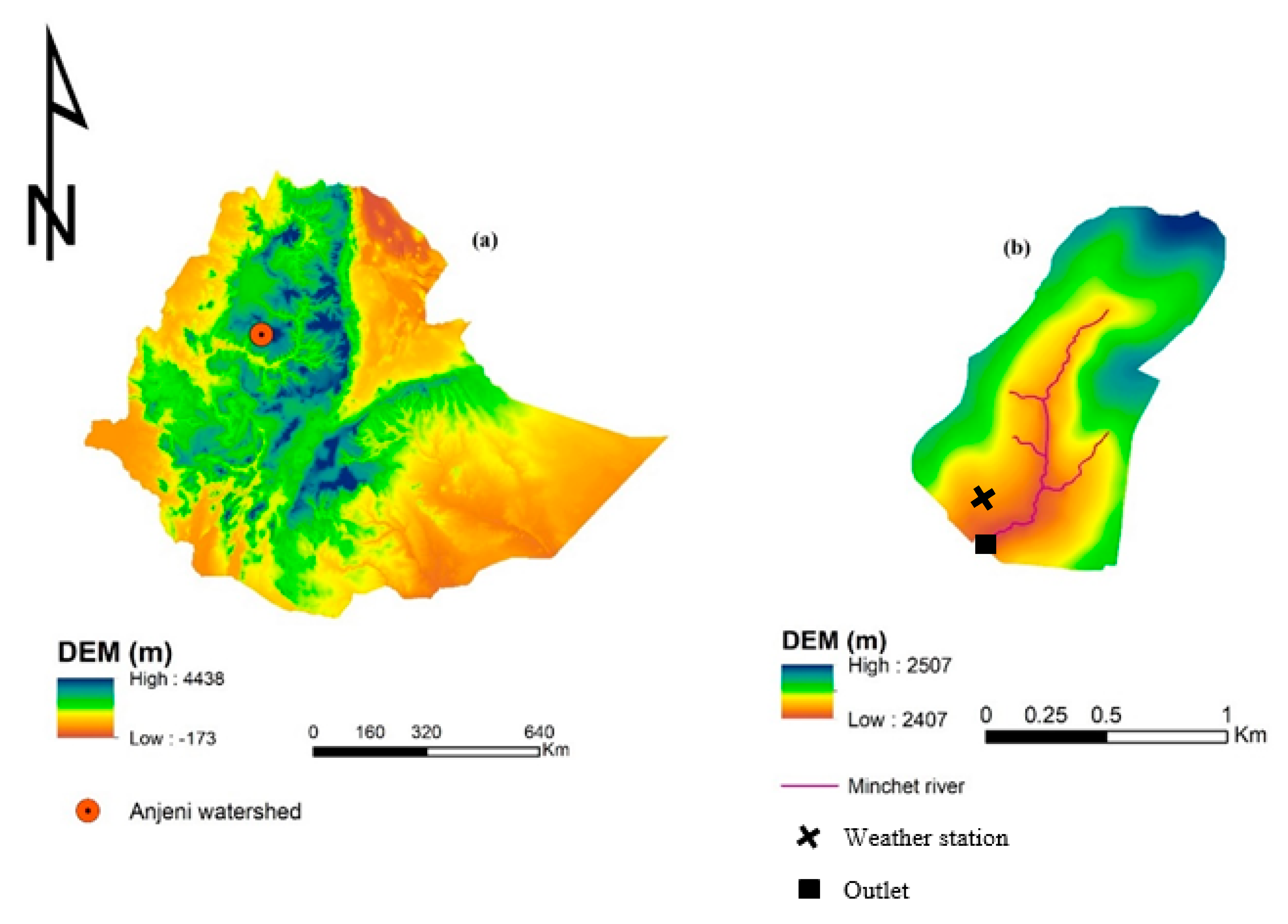
2.1. Study Site

This study was carried out in the Anjeni watershed, a small (113 ha) agricultural watershed, in the northwestern Ethiopian highlands (Figure 1). The Anjeni watershed was selected for this study because of the availability of long-term streamflow and sediment concentration records at its watershed outlet (Figure 1). In Ethiopia, continuous hydro-meteorological monitoring data are rarely available at a watershed scale to support hydrological process understanding. However, at Anjeni watershed, streamflow, sediment, and other watershed biophysical data were collected through the Soil Conservation and Research Program [26,27,28], which is a collaborative project between the Ethiopian Ministry of Agriculture and the Swiss Agency for Development and Cooperation (SDC). The watershed has been serving as a hydrological and erosion monitoring site under this program. Most of the watershed area (>80%) is covered with soils such as Alisols, Nitisols, and Cambisols that were developed from basalt and volcanic ash [29]. The bottom part of the watershed has relatively deeper Alisol soils; the mid and gentle slope parts of the watershed are covered by moderately deep Nitisols; while the steep slope and upper parts of the watershed have shallow Regosols and Leptosols [29]. On average, the watershed receives ~1600 mm rainfall. Daily average temperature ranges between 9 °C and 23 °C.

2.2. Data Inputs

2.2.1. Hydro-Climatic Data

The SWAT model requires daily climatic data to simulate watershed processes. Daily rainfall and maximum/minimum temperature data for the period 1984–1994 were used to set up the model. The rainfall and temperature data were obtained from a weather station near the outlet of the Anjeni watershed (Figure 2). The SWAT model also requires solar radiation, wind speed, and relative humidity data, which were generated from the Climate Forecast System Reanalysis data [30]. The watershed has a unimodal rainfall pattern and most of the rain occurs during the monsoon rainy season that lasts between June to September [28].

2.2.2. Streamflow and Sediment Data

Streamflow and sediment concentration data were monitored at the outlet of the Anjeni watershed. The streamflow has been measured continuously since 1984 [27]. Sediment concentration was monitored by grab-sampling 1 L water samples every 10- or 30-min interval. The sampling interval was decided based on the color change of the stream water. The total sediment load was calculated from sediment concentration in the water sample and the corresponding flow volume that was generated using the rating curve of the watershed. Detailed information about runoff and sediment measurements at the outlet of the Anjeni watershed are presented in Bayabil et al. [26,27].

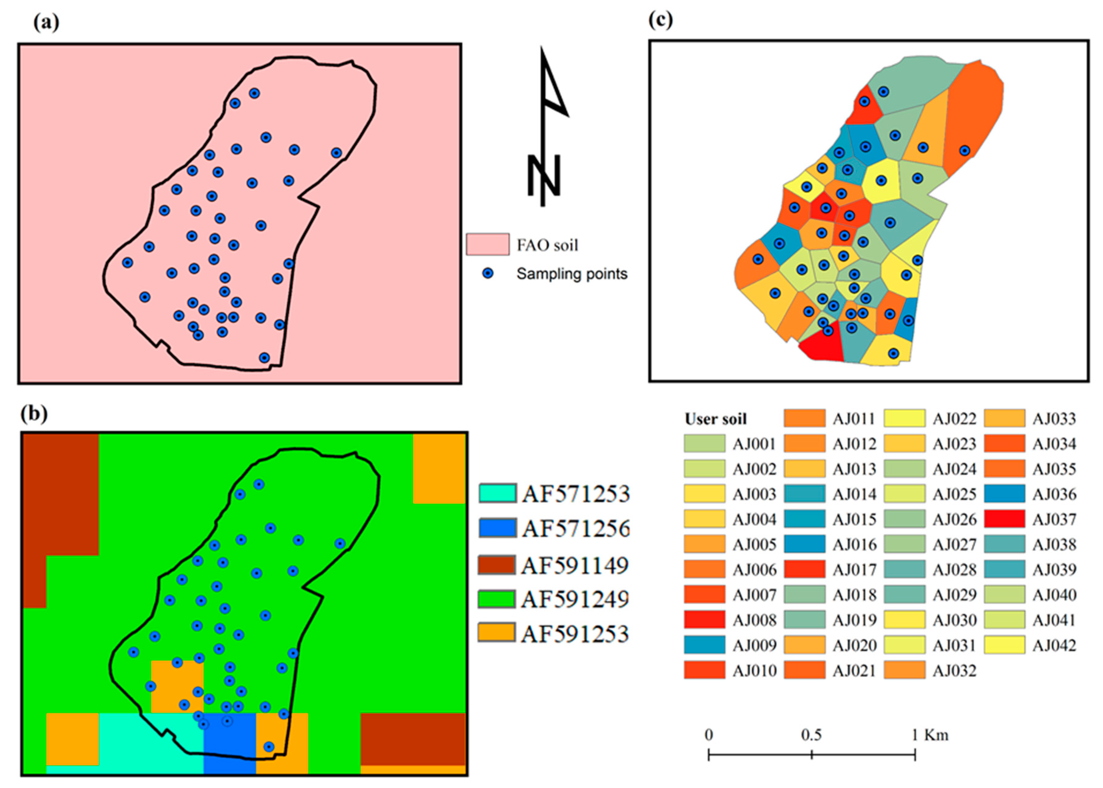
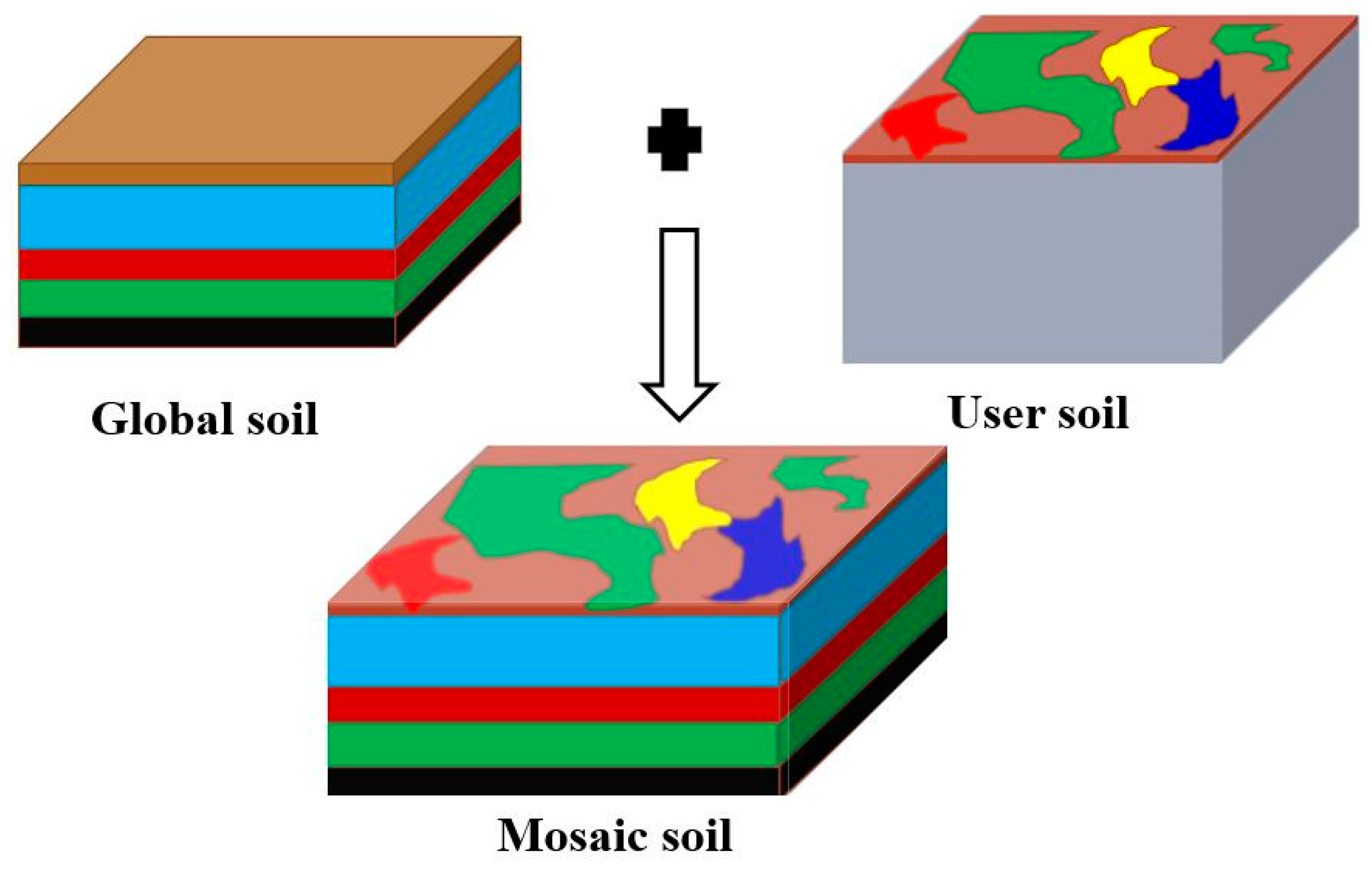
2.2.3. Soil Data Sources and Integration Approach

This study evaluated the simulation performance of five soil datasets: Three single sources obtained from field measurements (user soil), African Soil Information Service (AfSIS) [31], FAO Harmonized soil datasets [32], and two integrated soils produced by combining the user soil with the latter two.
The user soil dataset used in this study were previously used by Bayabil et al. [23,28]. The user soil database was developed based on field measurements at 42 locations in the Anjeni watershed by taking soil samples from the top 30 cm. Field soil measurements consisted of bulk density, infiltration, soil depth, soil texture, organic carbon content, and pH. Bayabil et al. [28] presented a detailed description of the soil physical and chemical properties and the measurement techniques used. Point-based soil information was used to develop a spatial soil map that covers the entire Anjeni watershed using the Thiessen polygon method in ArcGIS 10.4. The Thiessen polygon method generates polygons with one sampling point per polygon and assigns soil property values measured at a sampling point to the area within each polygon. As a result, 42 unique soil polygons were produced based on the same number of soil sampling points. The AfSIS data provide soil information at 250 m spatial resolution and contains most of the soil parameters for six soil layers [31,33], while the FAO dataset is available at 1 km resolution and has two layers [32]. Figure 2 presents the spatial coverage of AfSIS and FAO soils for the Anjeni watershed. The watershed is represented by a single soil type in the FAO soil dataset [32] and with four soil types in the AfSIS soil dataset (Figure 2).
The three soil datasets have different soil physical and hydraulic parameters. Summary of soil properties at different depths is presented in Table 1. Bayabil et al. [23] reported that the AfSIS and FAO datasets can provide a diverse estimate of soil parameters but fail to capture the spatial variability of actual field conditions. Moreover, they showed that user soils and global soils have their advantages and disadvantages in hydrologic modeling applications. Unlike the global soil databases, the user soil database has a finer resolution, but soil parameter measurements only for the top 30 cm. Therefore, two more datasets were created to leverage the finer resolution capabilities of the user soil and multiple layer information of the global soil datasets. The new soil datasets were created by replacing the top 30 cm soil information of the global datasets (AfSIS and FAO) by the soil parameters from the user soil. For example, an integration of a soil that has two layers at a certain location in the FAO soil and a respective soil in the user soil will result in a soil type that has a top layer with information from the user soil and a second layer with soil information from the FAO soil dataset (Figure 3). The study, therefore, used these five soil datasets to simulate the SWAT model and evaluate the performance of the soil datasets to simulate streamflow and sediment yield in a case study in the Anjeni watershed.

2.2.4. Land Use and Digital Elevation Model

Besides the soil data, land use, and digital elevation model (DEM) are basic spatial data required by the SWAT model to discretize the watershed and define the Hydrological Response Units (HRUs). The DEM and land use data were developed under the SCRP project. The DEM data have a spatial resolution of 2 m, which was helpful to accurately capture the river networks, developed by the Center for Development and Environment (CDE) at the University of Berne, Switzerland. The land use map was developed by recording crop type in each plot and fully represents field conditions.

2.3. SWAT Model Setup

The SWAT model discretization with a threshold area of one hectare provided 37 number of sub-basins. Three slope classes (i.e., <4, 4–8, >8%) were created for the Hydrologic Response Units (HRUs) formation. Multiple HRUs were created within a sub-basin. The model setup provided a total of 465, 201, and 164 HRUs from the User, AfSIS, and FAO soils, respectively.
SWAT has different options to calculate different biophysical processes in a watershed. This study used the Soil Conservation Service’s curve number (CN) method to estimate surface runoff. The Penman-Monteith method was used to calculate potential evapotranspiration. The routing of water in the channels was determined using the variable storage routing method.
The Soil and Water Assessment Tool (SWAT) model is a physically based watershed model with features that capture the spatial variability of biophysical parameters at Hydrological Response Unit (HRU) levels, which is the smallest unit in a watershed represented with similar land use, soil type, and elevation class. Although the model requires daily climate data, it can run at a daily or monthly timestep. SWAT has been used throughout the world to test various watershed related processes ranging from commonly used streamflow and sedimentation to nutrient transport, climate change, best management practices, chemical transport and cycling, and farming practices.
The SWAT model uses the following equation (Equation (1)) to simulate the water balance of a watershed [34].
S W t =   S W 0 + i = 1 t ( P i R i E T i W i Q i )
where SWt is final soil water content at time t (mm), SW0 is initial soil water content at time i (mm), t is time (days), Pi is the amount of precipitation on day i (mm), Ri is the amount of surface runoff on day i (mm), ETi is the amount of evapotranspiration on day i (mm), Wi is the percolation of water entering the vadose zone from the soil profile on day i (mm), and Qi is the amount of return flow on day i (mm).
Similarly, SWAT simulates sediment losses from a landscape due to rainfall and runoff using the Modified Universal Soil Loss Equation (MUSLE) developed by Williams [35], which is a modified version of the Universal loss Equation. Williams [35] used the following equation (Equation (2)).
S Y = 11.8 × ( R i × R p e a k × A h ) 0.56 × K × C × P × L S × C F R G
where SY is sediment yield (tons/day), Ri is surface runoff volume (mm/ha), Rpeak = peak runoff rate (m3/s), Ah is area of HRU (ha), and CFRG is coarse fragment factor. Meanwhile, the other parameters of the equation are based on the description by Wischmeier and Smith [36] and K is soil erodibility factor (0.013 ton m2 h)/(m3 tons cm), LS is length/slope factor, C is crop cover and management factor, and P is practice factor.

2.4. Model Calibration, Validation, and Sensitivity Analysis

A total of 12 model parameters were selected for streamflow calibration and validation, while for sediment calibration, 6 parameters were selected (Table 2). Model parameters considered for calibration were selected based on literature recommendation [14,37,38,39].
The SWAT model parameters were calibrated using the Sequential Uncertainty Fitting version 2 (SUFI-2) algorithm in the SWAT Calibration Uncertainty Prediction (SWAT-CUP) tool [40,41]. In SUFI-2, the level of uncertainty for a particular model is evaluated using p-factor and r-factor. The p-factor informs the percentage of observed data bracketed within the 95 percent prediction uncertainty (95 PPU) of the model while r-factor estimates the thickness of the 95 PPU. A p-factor close to 1 and an r-factor close to 0 suggest a reasonable level of model uncertainty [42]. The model was calibrated using observed streamflow and sediment data for the period 1988–1992 and 1990–1994, respectively. Model simulation for the period 1984–1987 was used for model warm-up. Daggupati et al. [43] recommend a model warm-up period of at least three years to properly initiate and balance stocks within the watershed. The model was validated using independently observed streamflow data for the period 1993–1994.
The evaluations of the model were conducted using the Nash-Sutcliffe Efficiency (NSE), which is a normalized statistic that determines the relative magnitude of the residual variance compared to the measured data variance [44]. An NSE value of 1 refers to a perfect match between observed and simulated values, and an NSE value between 0 and 1 is considered an acceptable level of model performance. An NSE value < 0 indicates that the observed mean is a better predictor than the model [45].

3. Results and Discussion

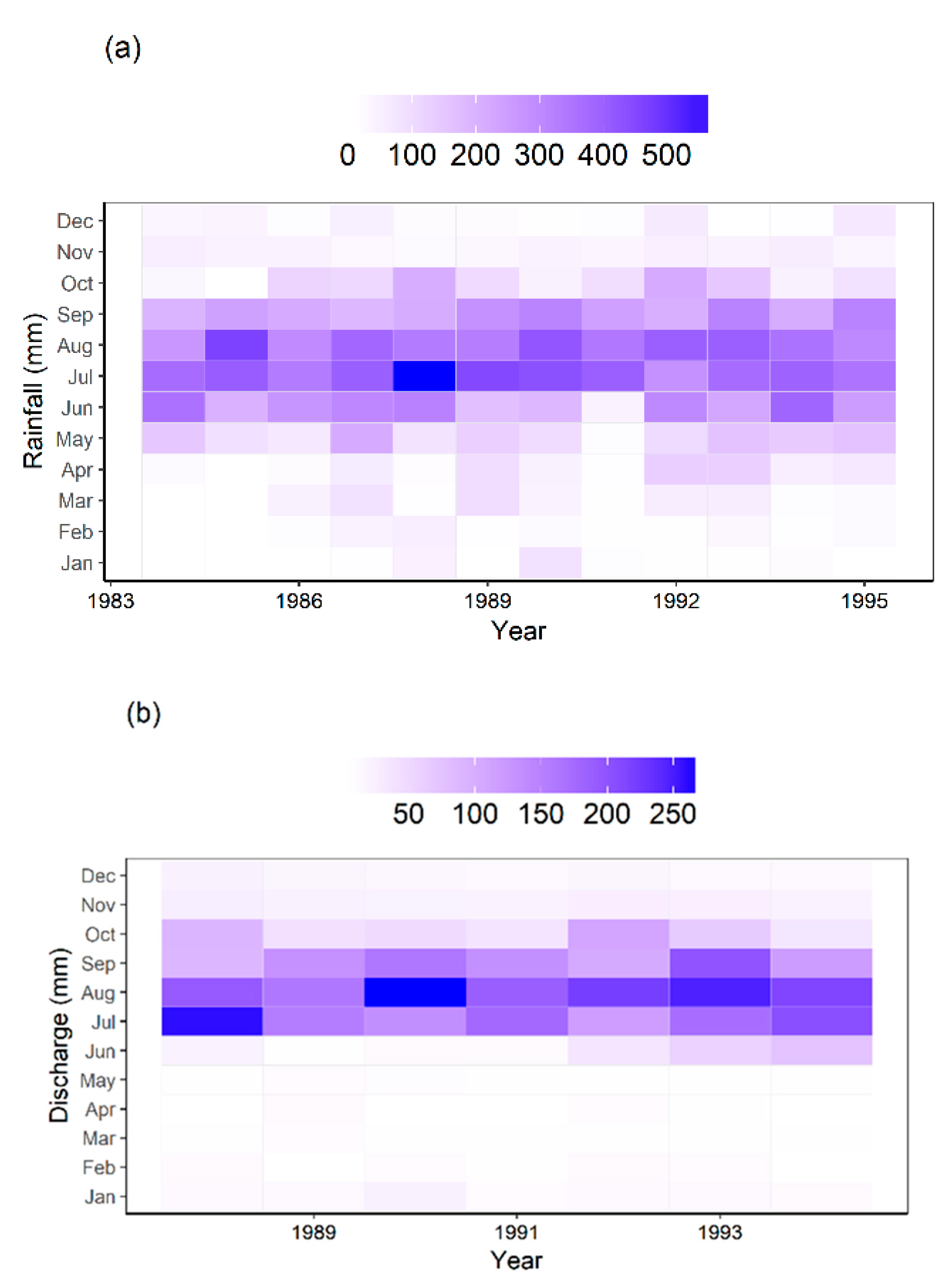
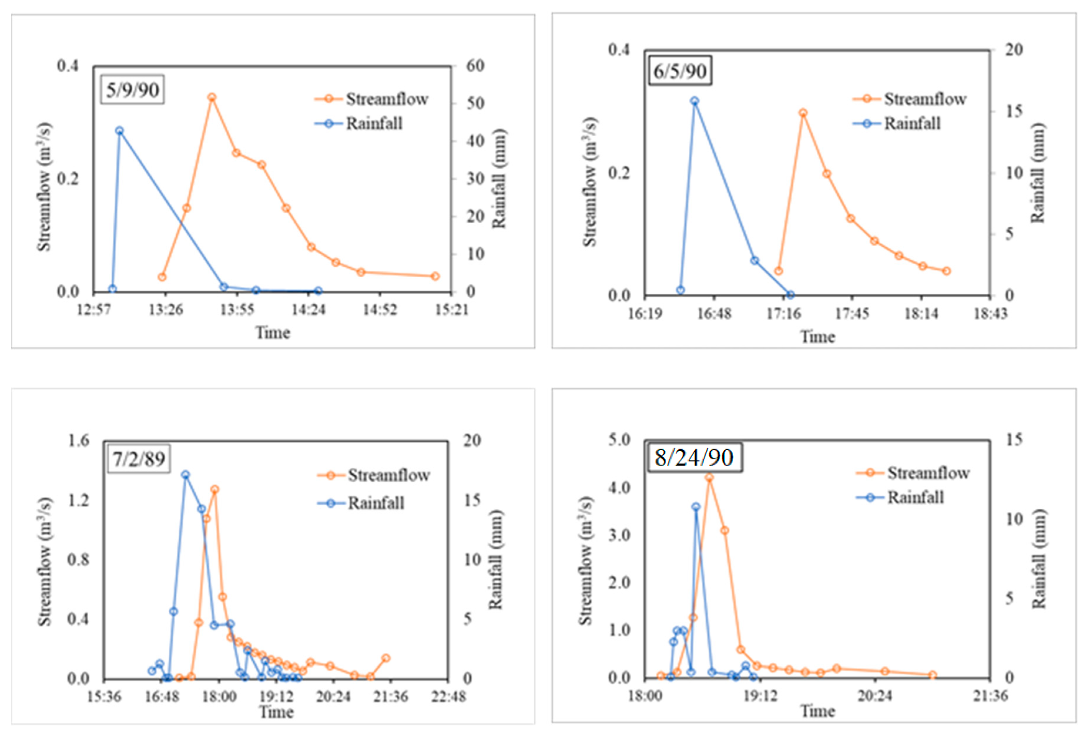
3.1. Long-Term Observed Rainfall, Discharge and Sediment Yield

Long-term data analysis showed that the Anjeni watershed receives an average annual rainfall of ~1600 mm and a runoff of ~700 mm. The average annual sediment yield was ~26.0 Mg ha−1. Since the watershed has a unimodal rainfall pattern, most of the streamflow and sediment losses occur during the rainy monsoon period of June to September (Figure 4). Sediment yield is greater towards the end of the rainy season, suggesting a significant contribution of gully erosion once the soils become saturated, perhaps at the bottom part of the watershed [3,5,46].
The average soil loss from the Anjeni watershed is smaller than the average erosion rate that Hurni (1988) estimated for the Ethiopian highlands (42 Mg ha−1); however, there are comparable sized watershed such as the Maybar watershed where the soil erosion is far lower at 7.4 Mg ha−1 [47]. Soil losses between 31 Mg ha−1 and 530 Mg ha−1 were reported in Ethiopian watersheds where severe gully erosion is prevalent [48].

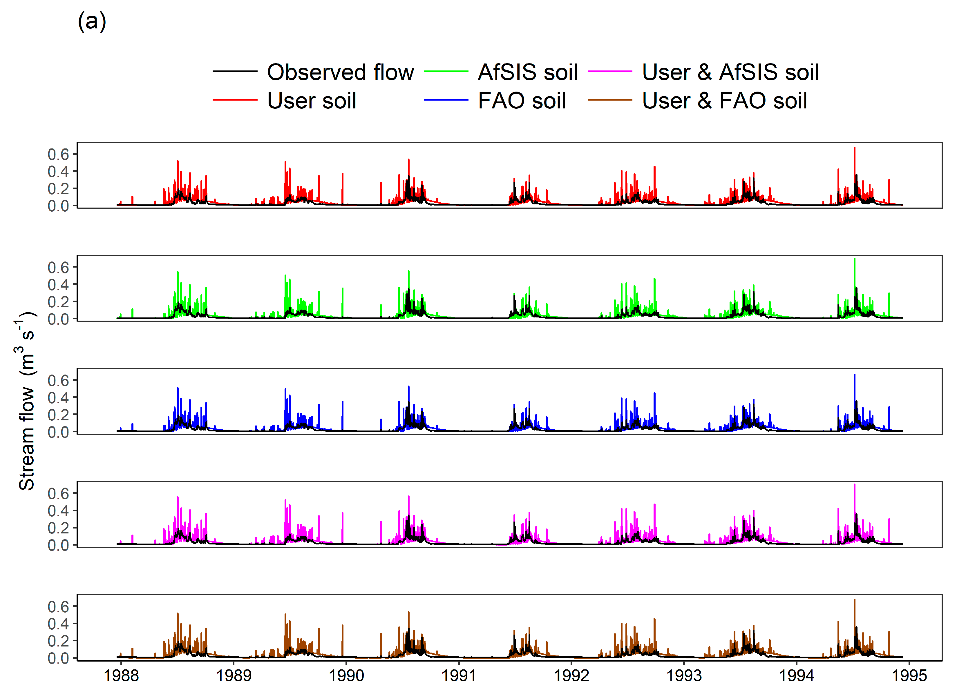
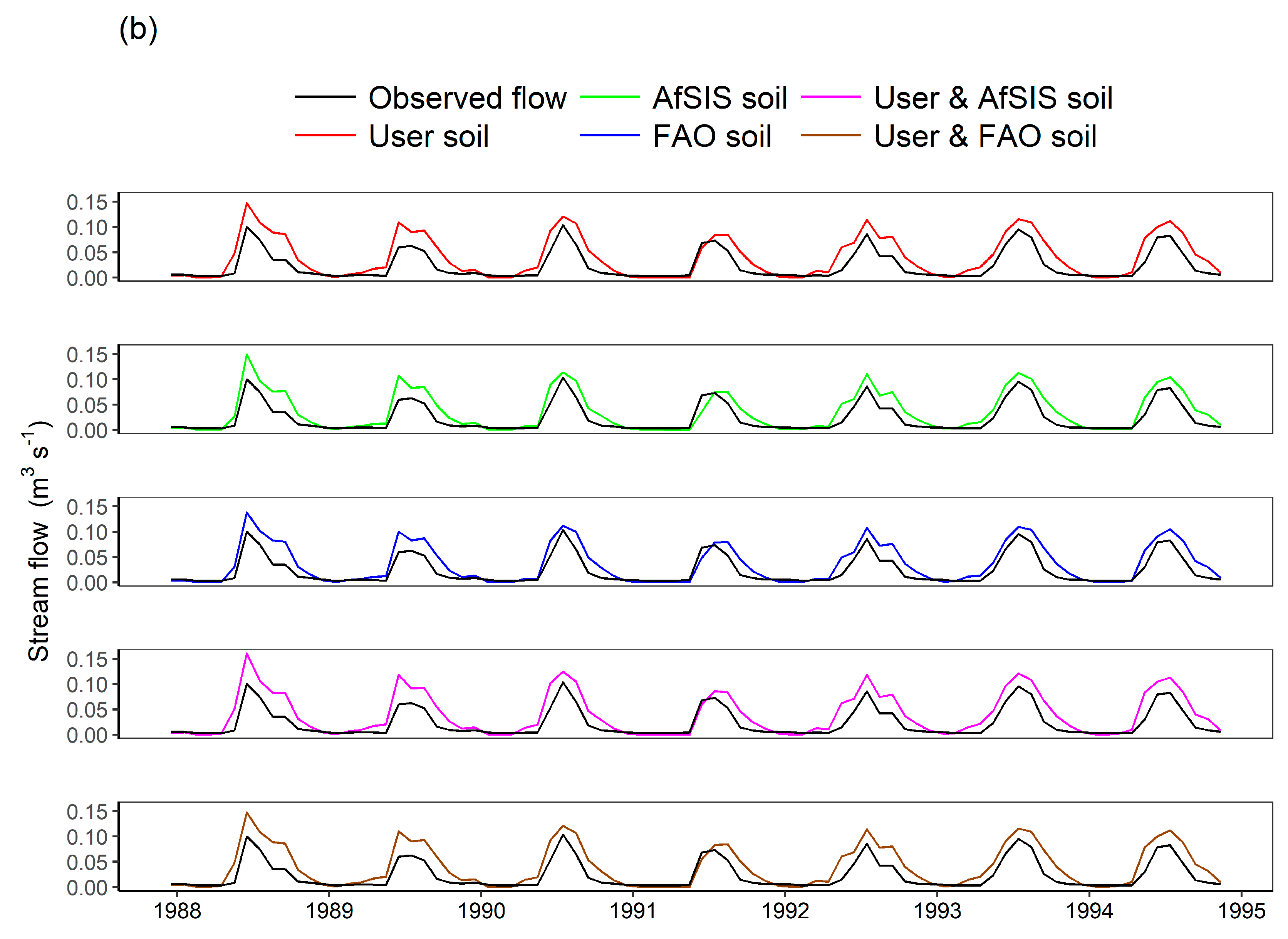
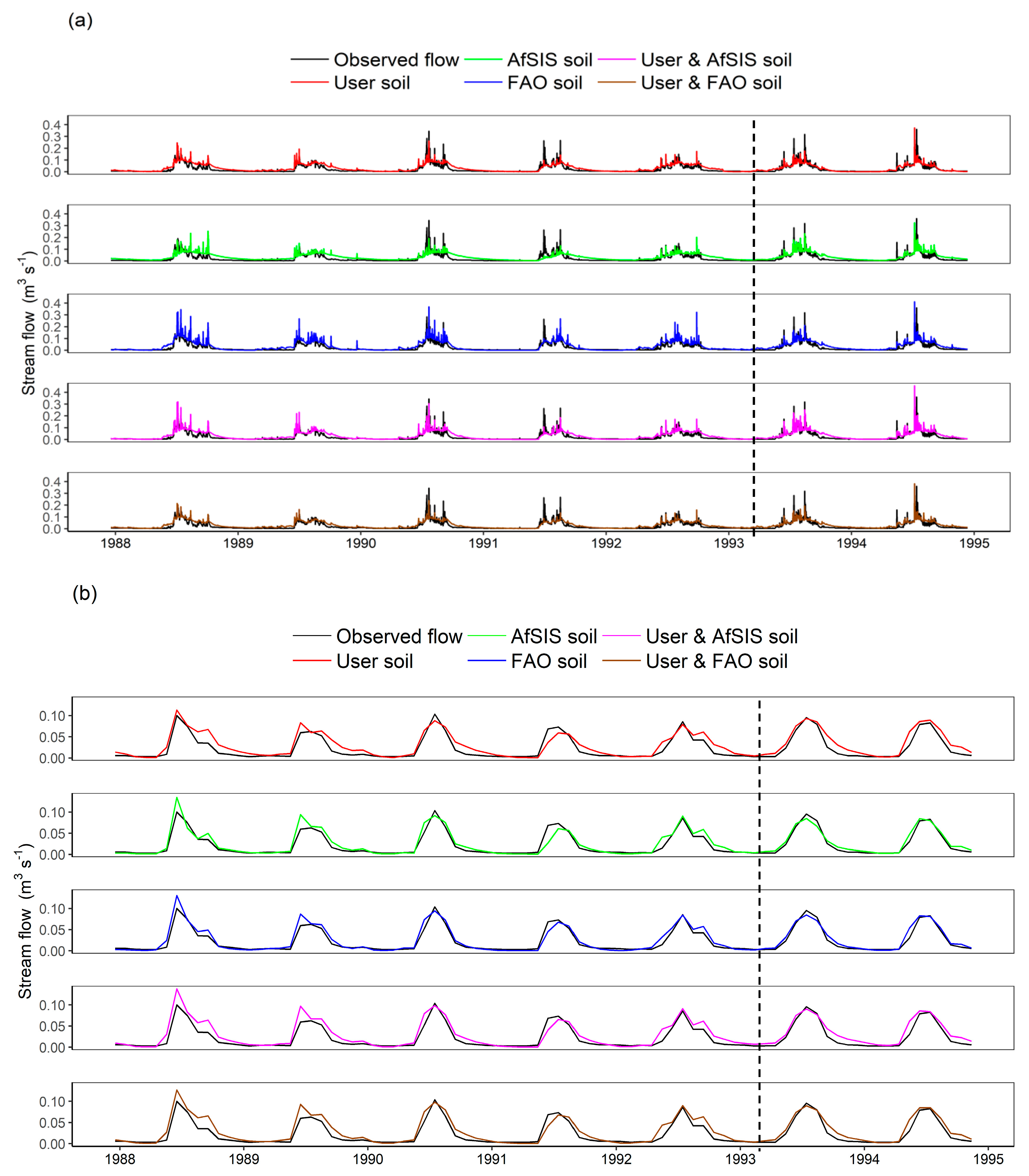
3.2. Effects of Soil Data Source on Streamflow Simulation

Uncalibrated model simulations from the five soil datasets (i.e., three independent and two integrated soil datasets) consistently overestimated streamflow at the Anjeni watershed both on daily and monthly time steps (Figure 5). While daily simulations appear to significantly overestimate peak and low flows (Figure 5a), the monthly simulations seem to follow the pattern of the observed hydrograph and capture low flows better (Figure 5b). Yet, the peak flows were significantly overestimated by all soil datasets even in the monthly simulations (Figure 5b).
It is a common practice to calibrate model parameters to mimic actual biophysical conditions in watersheds. Moreover, unsatisfactory model performance with the uncalibrated model parameters (Figure 5) suggested model calibration to fine-tune model parameters, thereby improving the streamflow simulation efficiency at the watershed outlet. Ayana et al. [49], without calibration, reported that AfSIS soils yield only marginal improvements in streamflow simulations compared to coarse resolution soil data inputs. In this study, the model calibration significantly improved streamflow simulations in the Anjeni watershed (Figure 6). Model calibration improved overestimation issues of the peak flows especially for monthly simulations (Figure 6b). Overall, the simulated streamflow hydrographs replicated the observed hydrographs well both during the calibration and validation periods (Figure 6).
Compared to the AfSIS and FAO soils, the user soil performed best in simulating the streamflow at a daily time step, while the AfSIS was the poorest. At daily time steps, the order of performance in terms of NSE goodness-of-fit evaluation is the user, AfSIS, and FAO soil datasets both during the calibration and validation periods (Table 3).
Replacing the top 30 cm information of AfSIS and FAO soils by information from the user soil greatly improved the model’s performance at daily time steps. Model performances of User-AfSIS and User-FAO datasets were better than their counterpart global soils (AfSIS and FAO) in stimulating daily streamflow, in which increases in NSE values for User-AfSIS and User-FAO simulations were 0.19 and 0.17 during model calibration, and 0.03 and 0.02% during model validation, respectively (Table 3). Similarly, reduction in PBIAS due to integration of the user soil with the AfSIS and FAO soils was 16 and 10% during model calibration, respectively. However, improvements due to soil data integration were better for the AfSIS soil compared to the FAO soil at daily simulations. Overall, based on Moriasi et al. [45] model performance scale, daily streamflow simulations have ‘very good’ ratings, except model simulations with the individual AfSIS and FAO soils which resulted in 0.45 and 0.55 NSE values during the model calibration period, respectively (Table 3).
At monthly time step, the user soil when used alone and integrated with the AfSIS and FAO soils did not improve streamflow simulations compared to the AfSIS and FAO soils (Table 3). The AfSIS and FAO soils when used independently provided better model performances for monthly streamflow simulations compared to user soil data both during calibration and validation. This suggests that the shallow depth in the measured User soil could not capture the relatively longer timestep water budget simulations. These findings have significant implications on the modeling and land and water management planning efforts in the region.
For example, for process understanding, which relies on analysis at daily- or sub-daily time steps in small watersheds, the use of detailed soil data at finer resolutions is warranted; however, for water balance studies, which is often conducted at monthly or annual scale, use of coarser resolution data that may have deeper soil profile may provide reasonable estimates. While this study showed that integrating fine resolution data into coarser global datasets improve model simulation performance at daily timestep, other studies have reported that the use of finer resolution soil datasets may not improve model performance. For example, Ye et al. [50], based on field observed soil data in a sub-humid watershed in China, reported that fine-resolution soil data inputs did not improve streamflow simulations at a larger watershed using the SWAT model. Similarly, Morias et al. [21] observed no significant differences in monthly streamflow prediction of fine and coarse resolution soil data inputs in their study at three sub-watersheds within the Fort Cobb Reservoir Experimental watershed in Oklahoma.
The Anjeni watershed has a very quick response time after storm events due to its short time of concentration; mostly less than one-hour even during dry months (Figure 7). This suggests that soil and water management planning that primarily intend to reduce runoff and sediment loss, and improve moisture availability for crop production, should rely on daily or sub-daily model simulations.
In the Anjeni watershed, monthly simulations are less promising for soil and water management planning purposes that are aimed to alleviate drought impacts on crop productivity. Since monthly simulations aggregate the daily hydrologic processes, it masks the daily variations of the water budget components (e.g., soil moisture, runoff). However, it requires balancing the intended uses of model outputs and scale of data resolution requirements (e.g., soil data) since data collection is costly, time-consuming, and at times impractical to cover large areas [23]. For example, [18] highlighted that the preparation of fine resolution soil data for model calibration requires greater efforts and suggested that the benefits of fine-resolution data should be weighed against the resources needed. Moreover, having high-resolution data may also increase the computational needs especially in larger watersheds [18,22]. For example, although Anjeni is a relatively small watershed (113 ha), the user soil resulted in almost three times the number of HRUs (465) compared to the FAO soil (164), while the AfSIS soil had 201 HRUs. This suggested that as the watershed size and data resolution increases, the number of HRUs will considerably increase, thereby requiring substantial computational resources and time to make simulations.

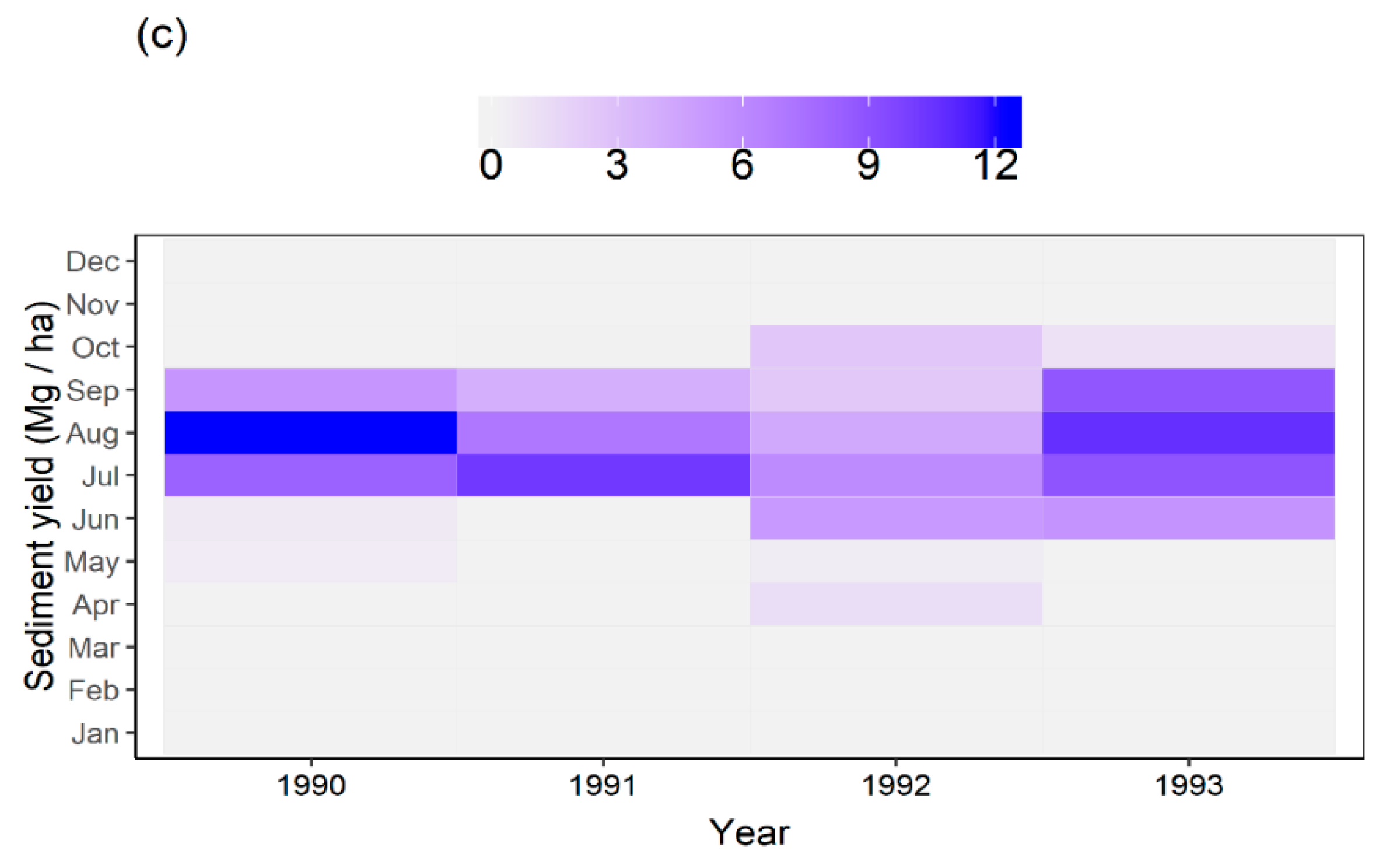
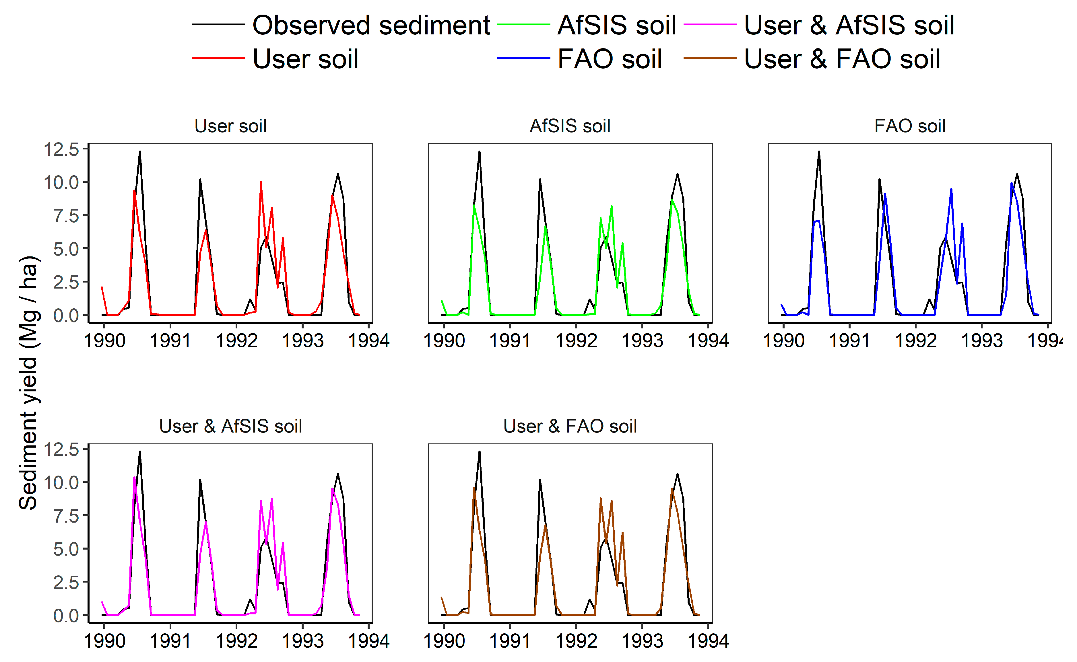
3.3. Effects of Soil Data Source on Sediment Yield Simulation

Similar to the streamflow simulation, the uncalibrated SWAT model could not effectively simulate sediment yield. The uncalibrated model substantially underestimated the peak sediment yield compared to the observed sediment yield. However, model calibration improved the sediment yield simulation (Figure 8). The NSE value for the sediment yield simulations with the different soil datasets varied between 0.72 and 0.77 (Table 4). Based on NSE values, all soil datasets performed similarly. According to Moriasi et al. [45], sediment yield simulations by the AfSIS soil dataset were ‘good’ while the user soil when integrated with the AfSIS soil provided a ‘very good’ model performance with NSE values of 0.77 (Table 4).
The user soil when used alone or integrated with the AfSIS and FAO soils provided better p-factor values (~0.26), which represents the percentage of data points bracketed within the 95PPU of the model simulations [42]. In contrast, the AfSIS and FAO soils provided lower p-factor values of 0.17 and 0.12 each. Although unsatisfactory p-values, the sediment yield simulations provided smaller r-factor values, which suggest a small level of model uncertainty. Abbaspour [42] suggested that a higher p-factor and smaller r-factor values suggest a smaller level of model uncertainty.
Regardless of the studied soil datasets, the sediment yield simulations were consistently underestimated compared to the observed sediment yield data. The average annual simulated sediment yield for the period 1990-1993 for the user, AfSIS, and FAO soils were 16.4, 18.2, and 15.8 Mg ha−1, respectively; while for the same period, the average annual observed sediment yield was 26.1 Mg ha−1. Underestimation of sediment yield simulation by the SWAT model was also reported in a similar sized Maybar watershed in the northern Ethiopian highlands [51]. The SWAT model’s consistent underestimation of peak sediment yield may be related to its limitations to account soil erosion from gullies. Field observations confirmed that active gully erosion exists in the Anjeni watershed and its contribution to total soil loss was found significant, especially once the soils become saturated [3,10,46]. Nyssen et al. [52] reported that gullying is among the dominant erosion processes in most areas in the Ethiopian highlands.

3.4. Water Budget

Annual precipitation and potential evapotranspiration were 1656 and 1160 mm, respectively. The simulated water yields with the AfSIS and FAO soil datasets were equal. The user soil, when used alone or integrated with the other two soils, estimated the highest water yield but the smallest actual evapotranspiration rates (AET) (Table 5). Smaller AET estimates for the user soil (and its integrated soils) suggested a more water limiting environment, which is more representative of the actual conditions in the Anjeni watershed than simulated by the other two soils. The AfSIS soil estimated the highest surface runoff when used alone and integrated with the user soil (Table 5). Transmission loss (TLoss) and groundwater revap did not show a significant difference among the soil dataset simulations.

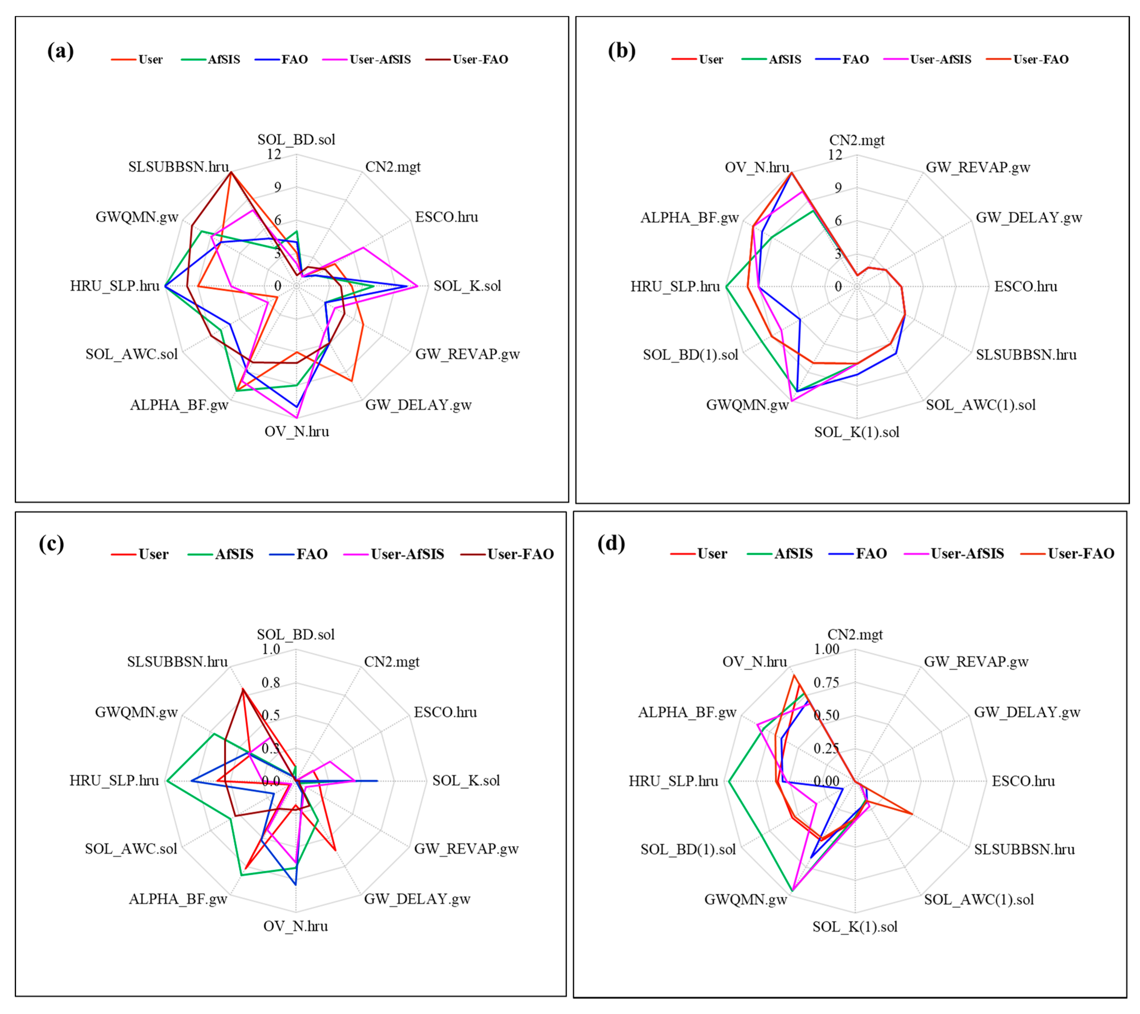
3.5. Sensitivity of Model Parameters

The curve number (CN) and soil bulk density (SOL_BD) were the top ranking and most sensitive model parameters to simulate streamflow using the three individual soils, and two user soil integrated with AfSIS and FAO soils (Figure 9). Overall, parameter rankings and sensitivity analysis showed that model parameters related to soil hydraulic properties were significantly sensitive in streamflow simulation, especially at daily time steps. Observed effects of integrating user soil with coarse resolution AfSIS and FAO soils were apparent on soil hydraulic parameters, which are known to affect hydrological processes at daily and sub-daily time steps. In contrast, however, model parameters related to groundwater showed higher ranking and sensitivity at monthly simulations since groundwater takes several days to respond. As a result, the ground water ‘revap’ coefficient (GW_REVAP) and groundwater delay (GW_DELAY) were the most sensitive parameters for monthly streamflow simulations. Based on field observations, soils in the study watershed are poorly managed and have compacted topsoil. Since surface runoff generation processes are primarily affected by hydrological parameters of the topsoil, the presence of such poorly managed top soils led to quick watershed response time. As such, daily simulations are appropriate to represent the actual hydrological processes in the watershed and thereby inform policy and management decisions related to soil and water conservation.

4. Conclusions

This study showed that the user soil, which has a finer spatial resolution, that better represents the spatial variability of soil hydrologic properties, improved hydrologic simulations when used independently or integrated with global soil datasets (AfSIS and FAO), especially at a daily time step. Moreover, this study showed that the integration of locally measured user soil data with global coarser resolution soil datasets (AfSIS and FAO) can enhance streamflow simulations, especially at a daily time step. However, the coarser resolution soil datasets such as the AfSIS and FAO soils could be effectively used to simulate monthly streamflow. This suggests that such coarse resolution soil datasets could be applicable for water balance studies in watersheds and sediment yield simulations, which are often performed at monthly or annual timescales. This study concluded that finer-resolution, locally collected soil datasets could be optimal for daily hydrologic simulations; however, freely available global soil datasets can also be integrated with locally measured soil information to achieve better hydrological simulations at daily time steps than the individual global soil counterparts. Hydrologic simulations should capture actual biophysical processes such as watershed response time, soil moisture dynamics, runoff generation, etc., as these factors are critical in soil and water management decision making. In rainfed farming systems, which are predominant in the study area, a few dry or wet days may have a significant impact on crop growth, yield, and produce quality. As such, field measured user soil’s finer resolution that helps daily hydrological processes understanding will play significant importance in soil and water management decisions.

Author Contributions

Conceptualization, H.K.B. and Y.T.D.; methodology, H.K.B. and Y.T.D.; data collection and analysis, H.K.B.; writing—original draft preparation, H.K.B.; writing—review and editing, H.K.B. and Y.T.D. All authors have read and agreed to the published version of the manuscript.

Funding

Funding for this research was partially provided by the University of Florida through the Early Career Scientist Seed Grant Award (#212-2100-00129077) and the Norman Borlaug Leadership Enhancement in Agriculture Program (LEAP). Yihun T. Dile’s time was made possible through support provided by the Feed the Future Innovation Lab for Small Scale Irrigation through the U.S. Agency for International Development, under the terms of Contract No. AID-OAA-A-13-0005. The opinions expressed herein are those of the authors and do not necessarily reflect the views of the U.S. Agency for International Development.

Conflicts of Interest

The authors declare no conflict of interest.

References

  1. Taddese, G. Land Degradation: A Challenge to Ethiopia. Environ. Manag. 2001, 27, 815–824. [Google Scholar] [CrossRef] [PubMed]
  2. Tebebu, T.Y.; Bayabil, H.K.; Steenhuis, T.S. Can degraded soils be improved by ripping through the hardpan and liming? A field experiment in the humid Ethiopian Highlands. Land Degrad. Dev. 2020, 1–13. [Google Scholar] [CrossRef]
  3. Tebebu, T.Y.; Bayabil, H.K.; Stoof, C.R.; Giri, S.K.; Gessess, A.A.; Tilahun, S.A.; Steenhuis, T.S. Characterization of degraded soils in the humid Ethiopian highlands. Land Degrad. Dev. 2016. [Google Scholar] [CrossRef] [Green Version]
  4. Tebebu, T.Y.; Steenhuis, T.S.; Dagnew, D.C.; Guzman, C.D.; Bayabil, H.K.; Zegeye, A.D.; Collick, A.S.; Langan, S.; MacAlister, C.; Langendoen, E.J.; et al. Improving efficacy of landscape interventions in the (sub) humid Ethiopian highlands by improved understanding of runoff processes. Front. Earth Sci. 2015, 3, 49. [Google Scholar] [CrossRef] [Green Version]
  5. Temesgen, M.; Uhlenbrook, S.; Simane, B.; van der Zaag, P.; Mohamed, Y.; Wenninger, J.; Savenije, H.H.G. Impacts of conservation tillage on the hydrological and agronomic performance of Fanya juus in the upper Blue Nile (Abbay) river basin. Hydrol. Earth Syst. Sci. 2012, 16, 4725–4735. [Google Scholar] [CrossRef] [Green Version]
  6. Feoli, E.; Gallizia, L.V.; Woldu, Z. Processes of Environmental Degradation and Opportunities for Rehabilitation in Adwa, Northern Ethiopia. Landsc. Ecol. 2002, 17, 315–325. [Google Scholar] [CrossRef]
  7. Dile, Y.T.; Tekleab, S.; Ayana, E.K.; Gebrehiwot, S.G.; Worqlul, A.W.; Bayabil, H.K.; Yimam, Y.T.; Tilahun, S.A.; Daggupati, P.; Karlberg, L.; et al. Advances in water resources research in the Upper Blue Nile basin and the way forward: A review. J. Hydrol. 2018, 560, 407–423. [Google Scholar] [CrossRef]
  8. Guzman, C.D.; Zimale, F.A.; Tebebu, T.Y.; Bayabil, H.K.; Tilahun, S.A.; Yitaferu, B.; Rientjes, T.H.M.; Steenhuis, T.S. Modeling discharge and sediment concentrations after landscape interventions in a humid monsoon climate: The Anjeni watershed in the highlands of Ethiopia. Hydrol. Process. 2017. [Google Scholar] [CrossRef]
  9. Liu, B.M.; Collick, A.S.; Zeleke, G.; Adgo, E.; Easton, Z.M.; Steenhuis, T.S. Rainfall-discharge relationships for a monsoonal climate in the Ethiopian highlands. Hydrol. Process. 2008, 22, 1059–1067. [Google Scholar] [CrossRef]
  10. Tilahun, S.A.; Guzman, C.D.; Zegeye, A.D.; Engda, T.A.; Collick, A.S.; Rimmer, A.; Steenhuis, T.S. An efficient semi-distributed hillslope erosion model for the subhumid Ethiopian Highlands. Hydrol. Earth Syst. Sci. 2013, 17, 1051–1063. [Google Scholar] [CrossRef] [Green Version]
  11. Dile, Y.T.; Srinivasan, R. Evaluation of CFSR climate data for hydrologic prediction in data-scarce watersheds: An application in the Blue Nile River Basin. Jawra J. Am. Water Resour. Assoc. 2018, 50, 1226–1241. [Google Scholar] [CrossRef]
  12. McMillan, H.; Gueguen, M.; Grimon, E.; Woods, R.; Clark, M.; Rupp, D.E. Spatial variability of hydrological processes and model structure diagnostics in a 50 km2 catchment. Hydrol. Process. 2014, 28, 4896–4913. [Google Scholar] [CrossRef]
  13. Bhandari, R.; Thakali, R.; Kandissounon, G.-A.A.-D.; Kalra, A.; Ahmad, S. Effects of Soil Data Resolution on the Simulated Stream Flow and Water Quality: Application of Watershed-Based SWAT Model. World Environ. Water Resour. Congr. 2018, 376–386. [Google Scholar] [CrossRef]
  14. Dile, Y.T.; Berndtsson, R.; Setegn, S.G. Hydrological Response to Climate Change for Gilgel Abay River, in the Lake Tana Basin—Upper Blue Nile Basin of Ethiopia. PLoS ONE 2013, 8, e79296. [Google Scholar] [CrossRef] [PubMed] [Green Version]
  15. Mizukami, N.; Clark, M.P.; Slater, A.G.; Brekke, L.D.; Elsner, M.M.; Arnold, J.R.; Gangopadhyay, S. Hydrologic Implications of Different Large-Scale Meteorological Model Forcing Datasets in Mountainous Regions. J. Hydrometeor. 2013, 15, 474–488. [Google Scholar] [CrossRef]
  16. Bitew, M.M.; Gebremichael, M.; Ghebremichael, L.T.; Bayissa, Y.A. Evaluation of High-Resolution Satellite Rainfall Products through Streamflow Simulation in a Hydrological Modeling of a Small Mountainous Watershed in Ethiopia. J. Hydrometeor. 2011, 13, 338–350. [Google Scholar] [CrossRef]
  17. Cotter, A.S.; Chaubey, I.; Costello, T.A.; Soerens, T.S.; Nelson, M.A. Water Quality Model Output Uncertainty as Affected by Spatial Resolution of Input Data. J. Am. Water Resour. Assoc. 2007, 39, 977–986. [Google Scholar] [CrossRef]
  18. Geza, M.; McCray, J.E. Effects of soil data resolution on SWAT model stream flow and water quality predictions. J. Environ. Manag. 2008, 88, 393–406. [Google Scholar] [CrossRef]
  19. Steenhuis, T.S.; Collick, A.S.; Easton, Z.M.; Leggesse, E.S.; Bayabil, H.K.; White, E.D.; Awulachew, S.B.; Adgo, E.; Ahmed, A.A. Predicting discharge and sediment for the Abay (Blue Nile) with a simple model. Hydrol. Process. 2009, 23, 3728–3737. [Google Scholar] [CrossRef]
  20. Chaubey, I.; Cotter, A.S.; Costello, T.A.; Soerens, T.S. Effect of DEM data resolution on SWAT output uncertainty. Hydrol. Process. 2005, 19, 621–628. [Google Scholar] [CrossRef] [Green Version]
  21. Moriasi, D.N.; Starks, P.J. Effects of the resolution of soil dataset and precipitation dataset on SWAT2005 streamflow calibration parameters and simulation accuracy. J. Soil Water Conserv. 2010, 65, 63–78. [Google Scholar] [CrossRef] [Green Version]
  22. White, K.L.; Chaubey, I. Sensitivity Analysis, Calibration, and Validations for a Multisite and Multivariable Swat Model1. Jawra J. Am. Water Resour. Assoc. 2005, 41, 1077–1089. [Google Scholar] [CrossRef]
  23. Bayabil, H.K.; Dile, Y.T.; Tebebu, T.Y.; Engda, T.A.; Steenhuis, T.S. Evaluating infiltration models and pedotransfer functions: Implications for hydrologic modeling. Geoderma 2019, 338, 159–169. [Google Scholar] [CrossRef]
  24. Saxton, K.E.; Rawls, W.J. Soil Water Characteristic Estimates by Texture and Organic Matter for Hydrologic Solutions. Soil Sci. Soc. Am. J. 2006, 70, 1569. [Google Scholar] [CrossRef] [Green Version]
  25. Arnold, J.G.; Moriasi, D.N.; Gassman, P.W.; Abbaspour, K.C.; White, M.J.; Srinivasan, R.; Santhi, C.; Harmel, R.D.; van Griensven, A.; van Liew, M.W.; et al. SWAT: Model Use, Calibration, and Validation. Trans. Asabe 2012, 55, 1491–1508. [Google Scholar] [CrossRef]
  26. Bayabil, H.K.; Yiftaru, B.; Steenhuis, T.S. Shift from transport limited to supply limited sediment concentrations with the progression of monsoon rains in the Upper Blue Nile Basin: Sediment Transportation in The Blue Nile Basin. Earth Surf. Process. Landf. 2017. [Google Scholar] [CrossRef]
  27. Bayabil, H.K.; Tebebu, T.Y.; Stoof, C.R.; Steenhuis, T.S. Effects of a deep-rooted crop and soil amended with charcoal on spatial and temporal runoff patterns in a degrading tropical highland watershed. Hydrol. Earth Syst. Sci. 2016, 20, 875–885. [Google Scholar] [CrossRef] [Green Version]
  28. Bayabil, H.K.; Stoof, C.R.; Lehmann, J.C.; Yitaferu, B.; Steenhuis, T.S. Assessing the potential of biochar and charcoal to improve soil hydraulic properties in the humid Ethiopian Highlands: The Anjeni watershed. Geoderma 2015, 243–244, 115–123. [Google Scholar] [CrossRef]
  29. Zeleke, G. Landscape Dynamics and Soil Erosion Process. Modelling in the North-Western Ethiopian Highlands; African Studies Series A 16; Geographica Bernensia: Bern, Switzerland, 2000. [Google Scholar]
  30. Saha, S.; Moorthi, S.; Pan, H.-L.; Wu, X.; Wang, J.; Nadiga, S.; Tripp, P.; Kistler, R.; Woollen, J.; Behringer, D.; et al. The NCEP Climate Forecast System Reanalysis. Bull. Am. Meteorol. Soc. 2010, 91, 1015–1057. [Google Scholar] [CrossRef]
  31. Hengl, T.; Heuvelink, G.B.M.; Kempen, B.; Leenaars, J.G.B.; Walsh, M.G.; Shepherd, K.D.; Sila, A.; MacMillan, R.A.; Mendes de Jesus, J.; Tamene, L.; et al. Mapping Soil Properties of Africa at 250 m Resolution: Random Forests Significantly Improve Current Predictions. PLoS ONE 2015, 10, e0125814. [Google Scholar] [CrossRef]
  32. Harmonized World Soil Database—Version 1.1; FAO: Rome, Italy, 2009; p. 43.
  33. Leenaars, J.G.B.; Claessens, L.; Heuvelink, G.B.M.; Hengl, T.; Ruiperez González, M.; van Bussel, L.G.J.; Guilpart, N.; Yang, H.; Cassman, K.G. Mapping rootable depth and root zone plant-available water holding capacity of the soil of sub-Saharan Africa. Geoderma 2018, 324, 18–36. [Google Scholar] [CrossRef] [PubMed]
  34. Neitsch, S.L.; Arnold, J.G.; Kiniry, J.R.; Williams, J.R. Soil and Water Assessment Tool Theoretical Documentation; Texas Water Resources Institute: Temple, TX, USA, 2011. [Google Scholar]
  35. Williams, J.R. Present and prospective technology for predicting sediment yield and sources. In Sediment-Yield Prediction with Universal Equation Using Runoff Energy Factor; U.S. Government Print Office: Washington, DC, USA, 1975; pp. 244–251. [Google Scholar]
  36. Wischmeier, W.H.; Smith, D.D. Predicting Rainfall Erosion Losses—A Guide to Conservation Planning; USDA, U.S. Government Print Office: Washington, DC, USA, 1978.
  37. Betrie, G.D.; Mohamed, Y.A.; van Griensven, A.; Srinivasan, R. Sediment management modelling in the Blue Nile Basin using SWAT model. Hydrol. Earth Syst. Sci. 2011, 15, 807–818. [Google Scholar] [CrossRef] [Green Version]
  38. Dile, Y.T.; Karlberg, L.; Srinivasan, R.; Rockström, J. Investigation of the Curve Number Method for Surface Runoff Estimation in Tropical Regions. Jawra J. Am. Water Resour. Assoc. 2016, 52, 1155–1169. [Google Scholar] [CrossRef]
  39. Setegn, S.G.; Dargahi, B.; Srinivasan, R.; Melesse, A.M. Modeling of Sediment Yield From Anjeni-Gauged Watershed, Ethiopia Using SWAT Model. Jawra J. Am. Water Resour. Assoc. 2010, 46, 514–526. [Google Scholar] [CrossRef]
  40. Abbaspour, K.C.; Johnson, C.A.; van Genuchten, M.T. Estimating Uncertain Flow and Transport Parameters Using a Sequential Uncertainty Fitting Procedure. Vadose Zone J. 2004, 3, 1340–1352. [Google Scholar] [CrossRef]
  41. Abbaspour, K.C.; Yang, J.; Maximov, I.; Siber, R.; Bogner, K.; Mieleitner, J.; Zobrist, J.; Srinivasan, R. Modelling hydrology and water quality in the pre-alpine/alpine Thur watershed using SWAT. J. Hydrol. 2007, 333, 413–430. [Google Scholar] [CrossRef]
  42. Abbaspour, K.C. SWAT-CUP: SWAT Calibration and Uncertainty Programs—A User Manual; Eawag: Dübendorf, Switzerland, 2015. [Google Scholar]
  43. Daggupati, P.; Pai, N.; Ale, S.; Doulgas-Mankin, K.R.; Zeckoski, R.; Jeong, J.; Parajuli, P.; Saraswat, D.; Youssef, M. A recommended calibration and validation strategies for hydrological and water quality models. Trans. Asabe 2015, 58, 1705–1719. [Google Scholar]
  44. Nash, J.E.; Sutcliffe, J.V. River flow forecasting through conceptualmodels: Part 1.—A discussion of principles. J. Hydrol. 1970, 10, 282–290. [Google Scholar] [CrossRef]
  45. Moriasi, D.N.; Arnold, J.G.; Van Liew, M.W.; Bingner, R.L.; Harmel, R.D.; Veith, T.L. Model Evaluation Guidlines for Systematic Quantification of Accuracy in Watershed Simulations. Trans. Asabe 2007, 50, 885–900. [Google Scholar] [CrossRef]
  46. Moges, M.A.; Zemale, F.A.; Alemu, M.L.; Ayele, G.K.; Dagnew, D.C.; Tilahun, S.A.; Steenhuis, T.S. Sediment concentration rating curves for a monsoonal climate: Upper Blue Nile. SOIL 2016, 2, 337–349. [Google Scholar] [CrossRef] [Green Version]
  47. Guzman, C.D.; Tilahun, S.A.; Zegeye, A.D.; Steenhuis, T.S. Suspended sediment concentration—Discharge relationships in the (sub-) humid Ethiopian highlands. Hydrol. Earth Syst. Sci. 2013, 17, 1067–1077. [Google Scholar] [CrossRef] [Green Version]
  48. Tebebu, T.Y.; Abiy, A.Z.; Zegeye, A.D.; Dahlke, H.E.; Easton, Z.M.; Tilahun, S.A.; Collick, A.S.; Kidnau, S.; Moges, S.; Dadgari, F.; et al. Surface and subsurface flow effect on permanent gully formation and upland erosion near Lake Tana in the northern highlands of Ethiopia. Hydrol. Earth Syst. Sci. 2010, 14, 2207–2217. [Google Scholar] [CrossRef] [Green Version]
  49. Ayana, E.K.; Dile, Y.T.; Narasimhan, B.; Srinivasan, R. Dividends in flow prediction improvement using high-resolution soil database. J. Hydrol. Reg. Stud. 2019, 21, 159–175. [Google Scholar] [CrossRef]
  50. Ye, X.; Zhang, Q.; Viney, N.R. The effect of soil data resolution on hydrological processes modelling in a large humid watershed. Hydrol. Process. 2011, 25, 130–140. [Google Scholar] [CrossRef]
  51. Yesuf, H.M.; Assen, M.; Alamirew, T.; Melesse, A.M. Modeling of sediment yield in Maybar gauged watershed using SWAT, northeast Ethiopia. CATENA 2015, 127, 191–205. [Google Scholar] [CrossRef]
  52. Nyssen, J.; Poesen, J.; Moeyersons, J.; Deckers, J.; Haile, M.; Lang, A. Human impact on the environment in the Ethiopian and Eritrean highlands—A state of the art. Earth Sci. Rev. 2004, 64, 273–320. [Google Scholar] [CrossRef]
Figure 1. Location of the study site in the Ethiopian highlands; Digital Elevation Model (DEM) maps of Ethiopia (a) and the DEM map of Anjeni watershed (b). The red circle with a black outline indicates the location of the Anjeni Map in Ethiopia.
Water 12 02763 g001
Figure 2. Maps of different soil data sources: (a) Food and Agriculture Organization (FAO) soil dataset, (b) Africa Soil Information Service (AfSIS) soil database, and (c) user soil developed based on 42 filed sampling points.
Water 12 02763 g002
Figure 3. Schematics of soil data integration.
Water 12 02763 g003
Figure 4. Long-term monthly average rainfall (a), discharge (b), and sediment yield records (c) at the Anjeni watershed.
Water 12 02763 g004aWater 12 02763 g004b
Figure 5. Comparison of measured and simulated streamflow before model calibration at the watershed outlet. Daily simulations (a) and monthly simulations (b).
Water 12 02763 g005aWater 12 02763 g005b
Figure 6. Comparison of measured and simulated streamflow after model calibration at the watershed outlet. Daily simulations (a) and monthly simulations (b). The vertical lines divide model calibration (left) and validation (right) periods.
Water 12 02763 g006
Figure 7. Event rainfall-runoff relationships for selected storm events from the Anjeni watershed.
Water 12 02763 g007
Figure 8. Comparison of observed and simulated monthly sediment yield at the outlet of Anjeni watershed. The simulated sediment yield plots are for the calibrated model parameters.
Water 12 02763 g008
Figure 9. Sensitivity analysis of SWAT model calibration parameters based on the five soil datasets (a,b) parameter rank and (c,d) t-statistics p-values for daily and monthly calibrations, respectively.
Water 12 02763 g009
Table 1. Summary of soil physical and hydrologic properties at different depths for the user (1 depth), AfSIS (7 depths), and FAO soil databases (2 depths). ρd, AWC, and Ks refer to bulk density, available water holding capacity, and hydraulic conductivity, respectively. Clay, Silt, and Sand refer to percentage textural classes.
ρd (g cm−3)AWC (cm3 cm−3)Ks (mm h−1)Clay (%)Silt (%)Sand (%)
Depth
(m)
UserAfSISFAOUserAfSISFAOUserAfSISFAOUserAfSISFAOUserAfSISFAOUserAfSISFAO
0.05 1.1 0.1 2.9 44 30 26
0.15 1.1 0.1 2.3 44 30 26
0.20
0.301.31.11.30.250.10.21.21.68.1414643342931252526
0.60 1.1 0.1 0.8 53 25 22
1.00 1.11.2 0.10.2 0.612.4 5454 2425 2221
2.00 1.1 0.1 0.5 55 23 22
Table 2. Selected flow and sediment calibration parameters and their ranges.
DescriptionValue Range
Flow parameters
r__CN2.mgtSCS runoff curve number±0.15
v__ALPHA_BF.gwBase-flow alpha factor (1/days) 0.0–1.0
a__GW_DELAY.gwGroundwater delay (days) −25–100
a__GWQMN.gwThreshold depth of water in the shallow aquifer required for return flow to occur (mm)0.0–1000
a__GW_REVAP.gwGroundwater “revap” coefficient0.0–0.18
v__ESCO.hruSoil evaporation compensation factor0.5–1.0
r__SOL_AWC.solAvailable water capacity of the soil layer (mm H2O/mm soil)±0.1
r__SOL_K.solSaturated hydraulic conductivity (mm/h)±0.1
r_SOL_BDSoil bulk density (g/cm3)±0.2
r_HRU_SLPAverage slope steepness (m/m)−0.1–0.15
r__OV_N.hruManning’s “n” value for overland flow−0.1–0.15
r__SLSUBBSN.hruAverage slope length (m)−0.1–0.15
Sediment parameters
v__USLE_P.mgtUSLE equation support practices0–1.0
v__SPCON.bsnLinear parameter for calculating the maximum amount of sediment that can be re-entrained during channel sediment routing.0.0001–0.1
v__SPEXP.bsnExponent parameter for calculating sediment re-entrained in channel sediment routing1.0–1.5
v__CH_COV1.rteChannel erodibility factor.−0.05–0.6
v__CH_COV2.rteChannel cover factor.0–1
v__USLE_C.plant.datMin value of USLE C factor applicable to the land cover/plant0.001–0.5
where qualifiers “a_”, “v_” and “r_” represent absolute increase, replacement, and relative change to the original parameter values, respectively.
Table 3. Evaluation measures for daily and monthly streamflow simulations using different soil datasets.
TimeSetupSoilNSEr2p-Factorr-FactorPBIAS
DailyCalUser0.650.730.430.48−40
CalAfSIS0.450.570.861.07−49
CalFAO0.550.680.110.08−41
CalUser-AfSIS0.640.720.270.26−33
CalUser-FAO0.720.770.500.51−31
ValUser0.780.770.350.47−37
ValAfSIS0.720.730.870.74−43
ValFAO0.710.750.900.98−21
ValUser-AfSIS0.750.790.380.35−32
ValUser-FAO0.730.770.190.36−29
MonthlyCalUser0.780.850.780.89−30
CalAfSIS0.840.880.870.83−13
CalFAO0.900.930.900.93−12
CalUser-AfSIS0.780.890.770.75−30
CalUser-FAO0.790.890.800.90−30
ValUser0.830.930.830.70−37
ValAfSIS0.950.960.920.42−11
ValFAO0.950.950.960.49−9
ValUser-AfSIS0.880.940.670.39−31
ValUser-FAO0.900.950.790.51−24
Table 4. Summary of Soil and Water Assessment Tool (SWAT) model performance in simulating monthly sediment yield using different soil datasets at the outlet of the Anjeni watershed.
Soil TypeNSEr2p-Factorr-FactorPBIAS
User0.720.720.380.455.0
AfSIS0.740.750.270.2013.5
FAO0.720.720.310.4610.2
User & AfSIS0.770.770.440.504.8
User & FAO0.740.740.380.465.3
Table 5. Summary of simulated water balance components for different soil types.
ParameterUser SoilUser-AfSISUser-FAOAfSISFAO
Water yield1205.31201.11200.31073.71073.7
AET428.7432.8433.7560.7560.6
Surf_Q594.5680.0593.0640.7554.3
GW_Q550.5441.3540.7388.4457.3
Perc573.4464.2563.6411.1480.2
Lat_Q60.379.766.644.762.1
where Water yield is average annual water leaving the watershed (mm), AET is actual evapotranspiration (mm), Surf_Q is surface runoff (mm), GW_Q is Deep aquifer groundwater contribution to streamflow (mm), Perc is water that percolates past the root zone (mm), and Lat_Q is lateral flow (mm).

