Method Consideration of Variation Diagnosis and Design Value Calculation of Flood Sequence in Yiluo River Basin, China

Abstract
1. Introduction
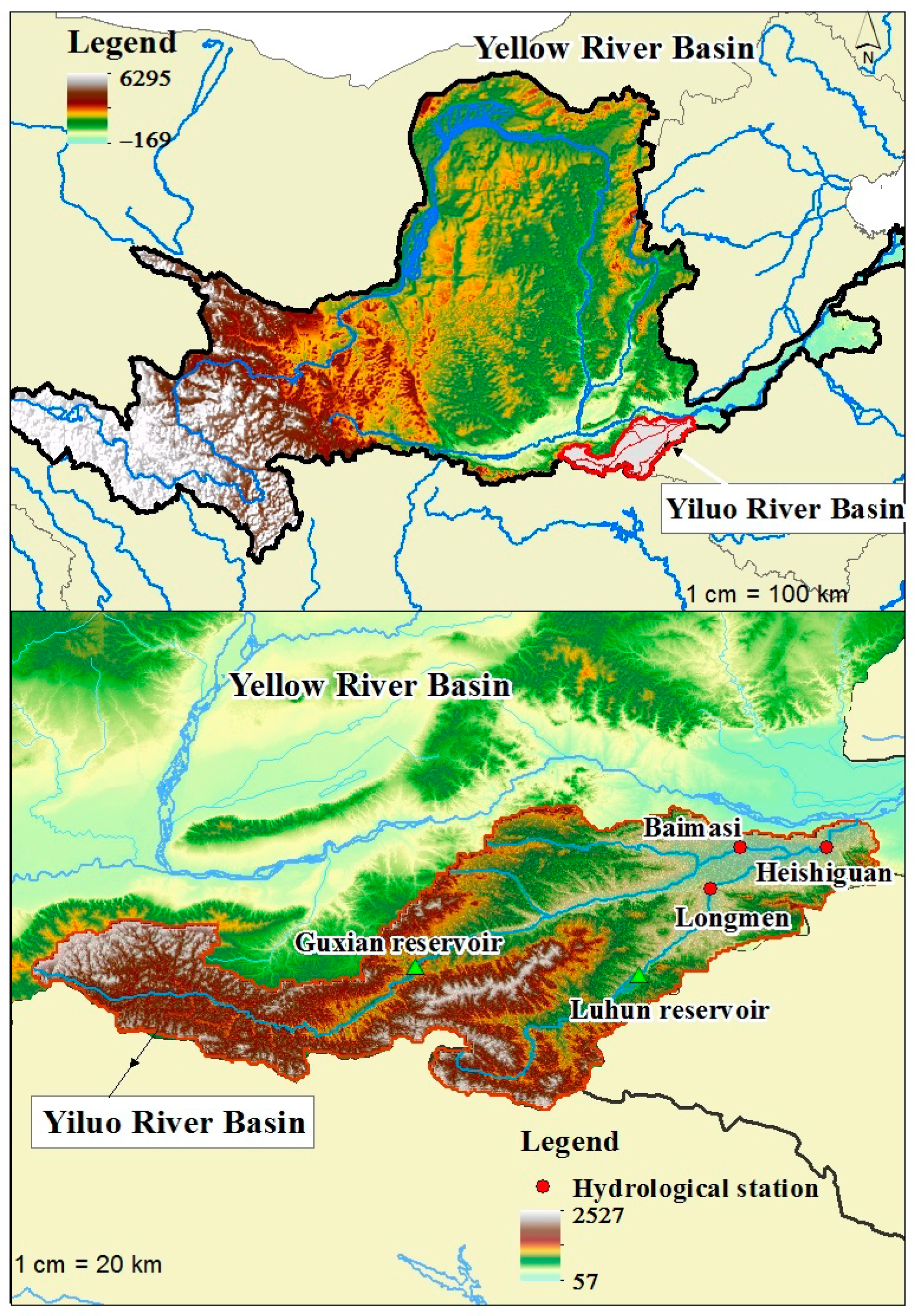
2. Study Area
3. Data
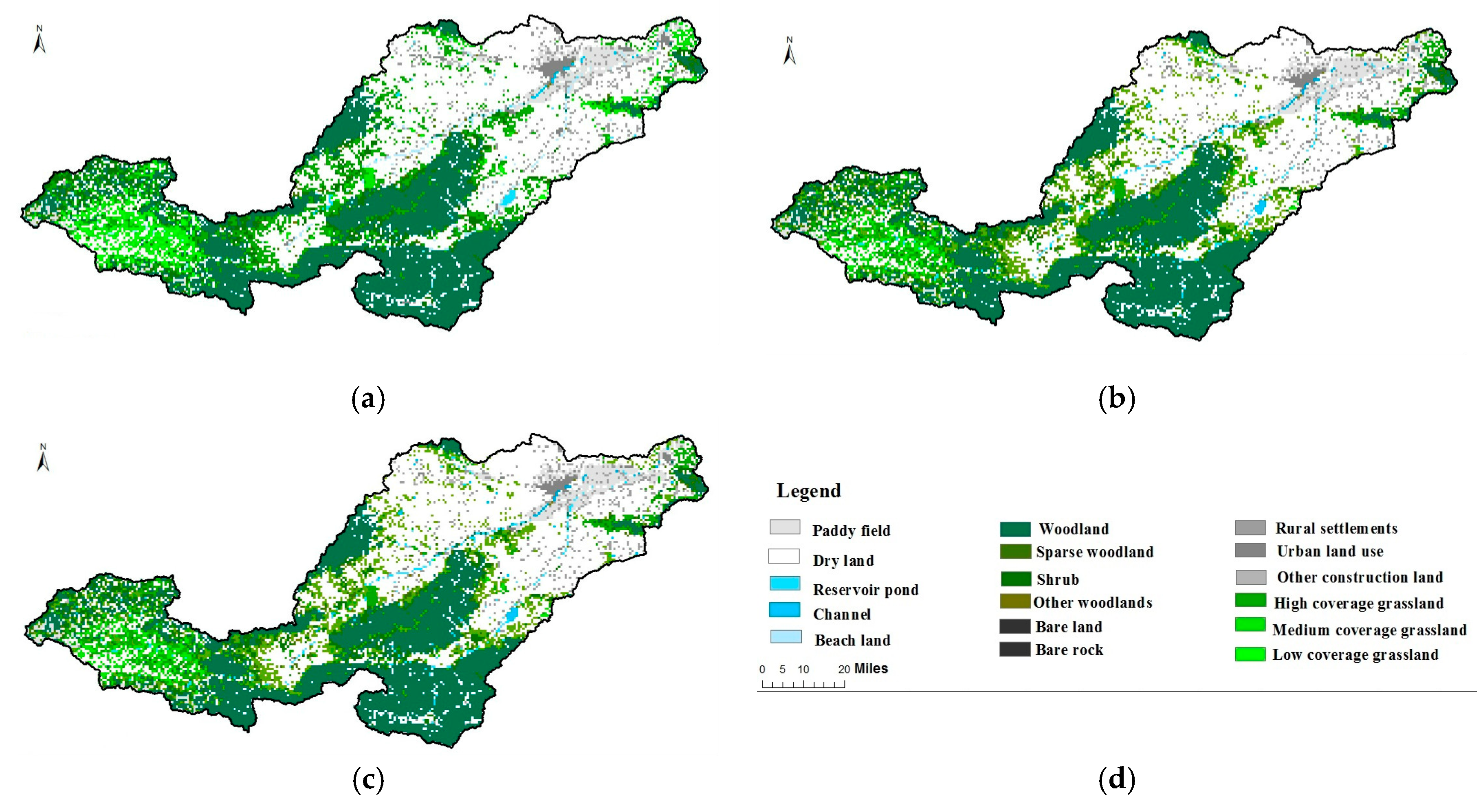
3.1. Basin Underlying Surface Data
3.2. Hydrometeorological Data
4. Methodology
4.1. Trend Detection Method
4.1.1. Linear Trend Test
4.1.2. Mann–Kendall Test
4.2. Jumping Detection Method
4.2.1. Hurst Index Method
4.2.2. Sliding T Test
4.2.3. Pettitt Test
4.3. Frequency Analysis
4.3.1. Time Series Decomposition-Synthesis Method
4.3.2. Mixed Distribution Model
5. Results and Discussion
5.1. Variation Diagnosis
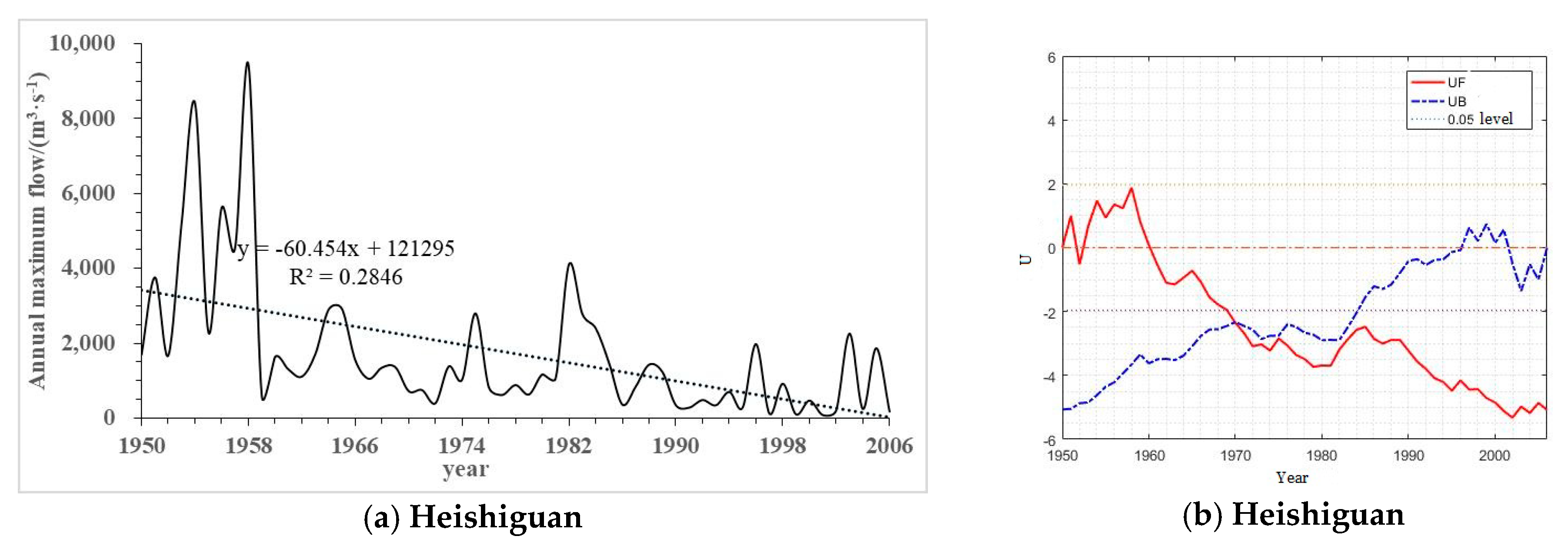
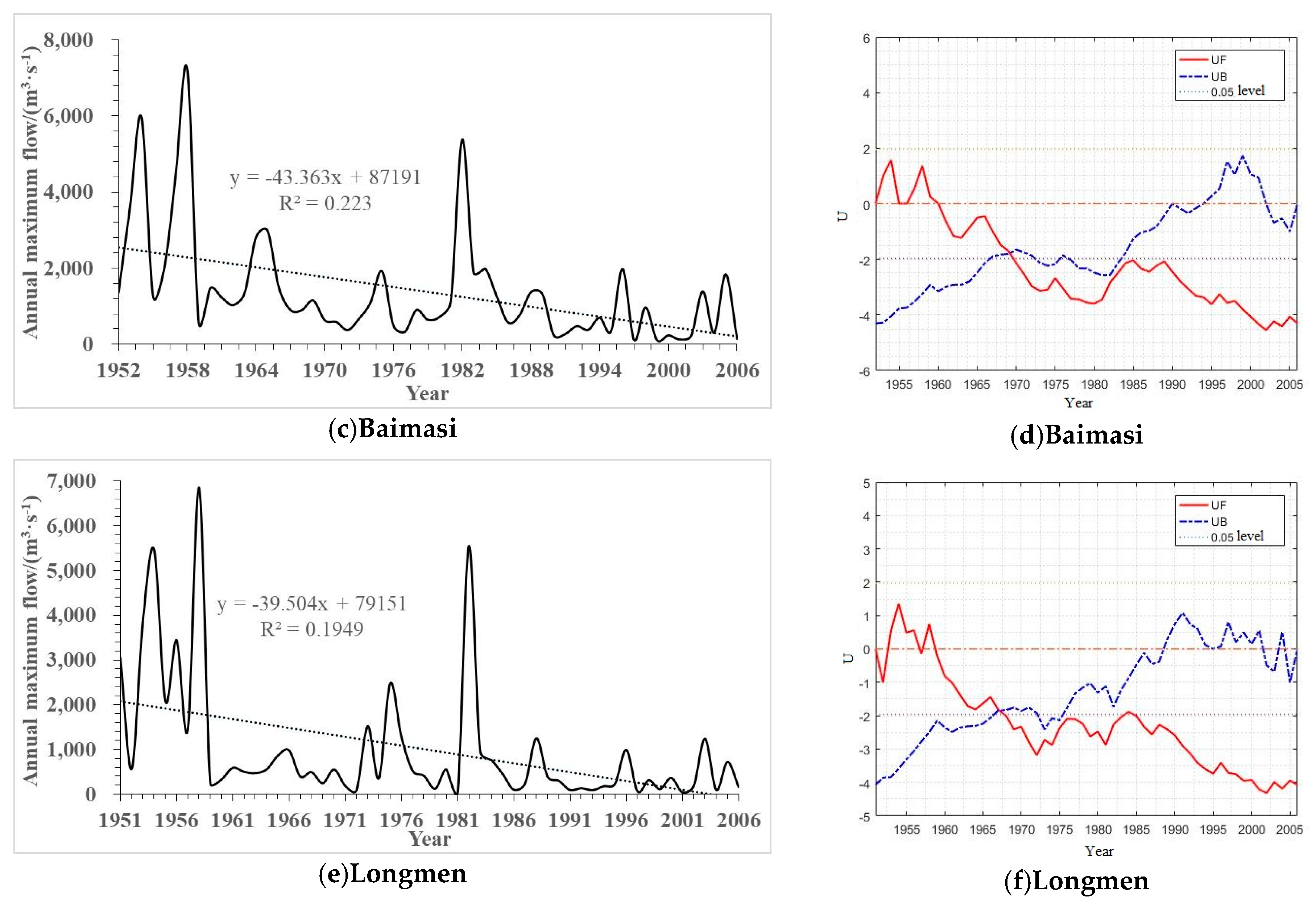
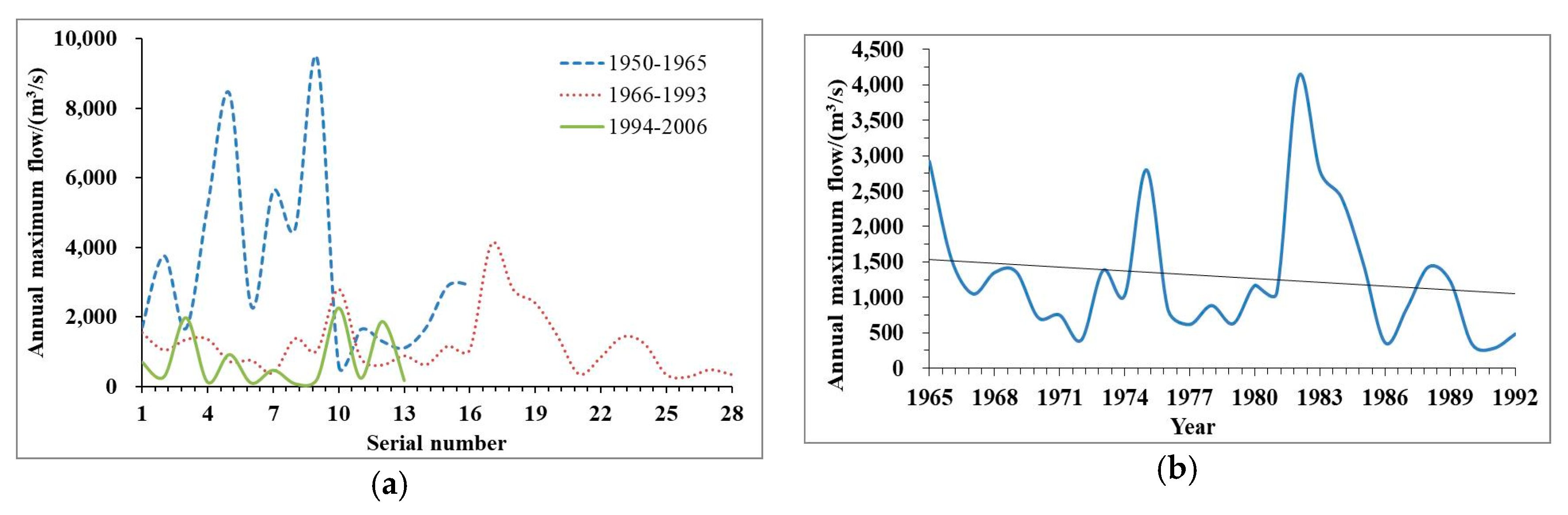
5.1.1. Trend Diagnosis
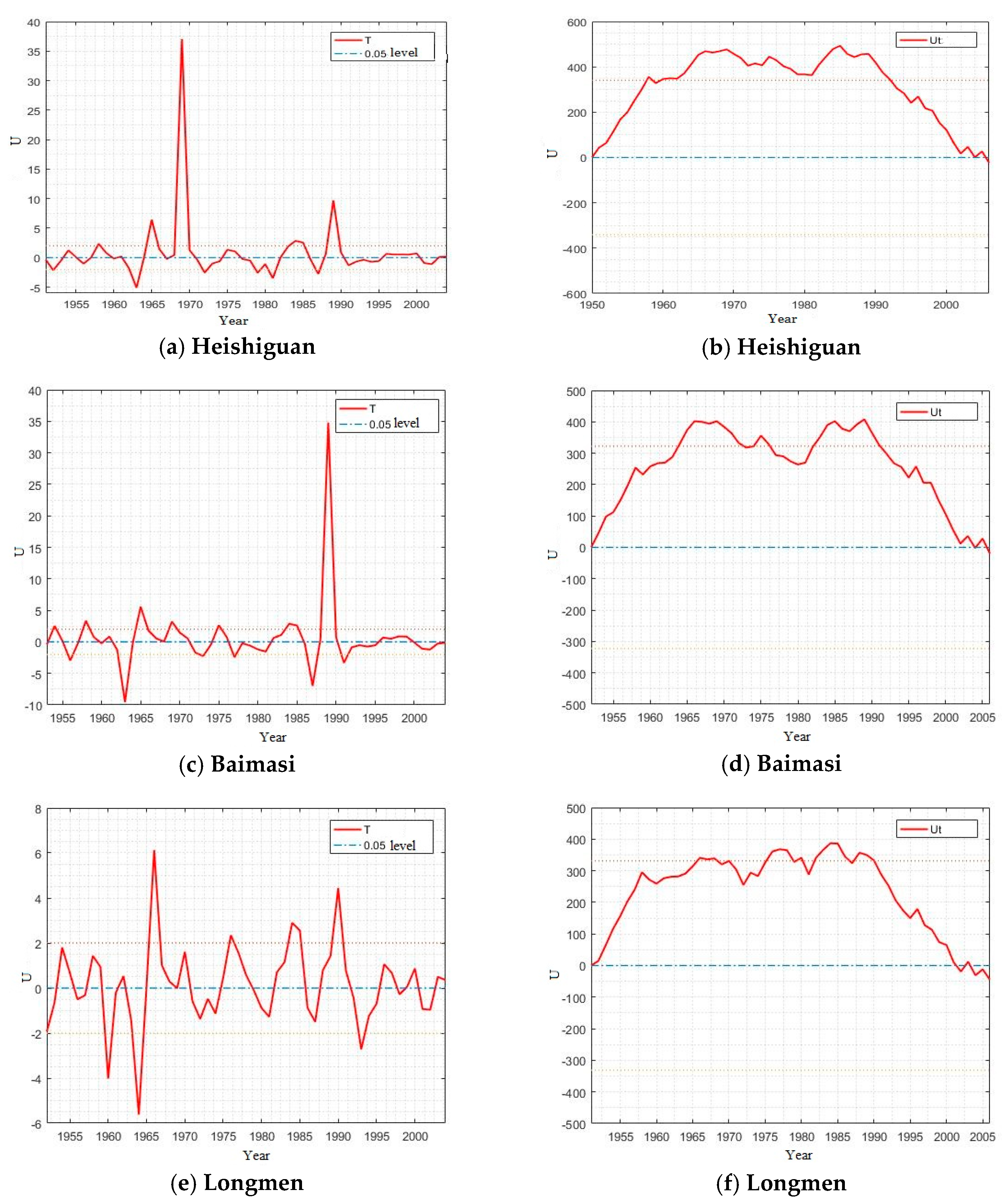
5.1.2. Jump Diagnosis
5.1.3. Combination of Variation Diagnosis
5.2. Design Value
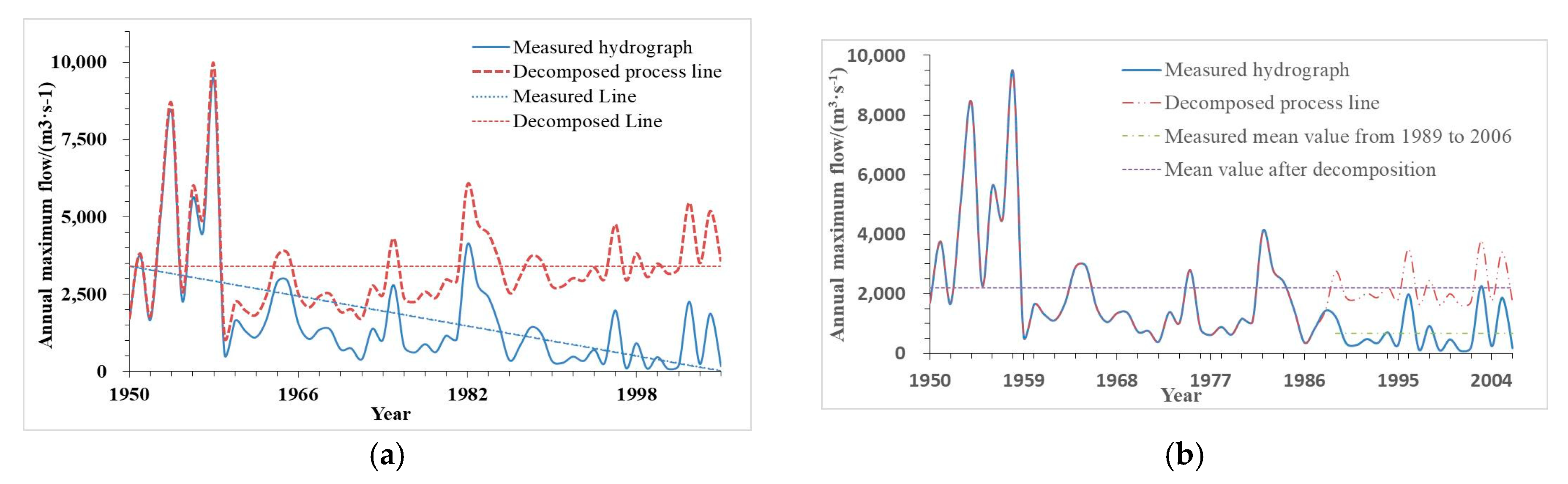
5.2.1. Time Series Decomposition Synthesis
5.2.2. Mixed Distribution Model
5.2.3. Design Value Analysis
6. Conclusions
Author Contributions
Funding
Conflicts of Interest
References
- Guo, S.; Liu, Z.; Xiong, L. Research progress and evaluation of design flood calculation method. J. Water Conserv. 2016, 47, 302–314. [Google Scholar]
- Mulvaney, T.J. On the use of self-registering rain and flood gauges in making observations of the relations of rainfall and flood discharges in a given catchment. Proc. Inst. Civ. Eng. Irel. 1851, 4, 19–31. [Google Scholar]
- Kuichling, E. The relation between the rainfall and the discharge of sewers in populous areas. Trans. Am. Soc. Civ. Eng. 1889, 20, 1–56. [Google Scholar]
- Chow, V.T.; Maidment, D.R.; Mays, L.W. Applied Hydrology; McGraw Hill: New York, NY, USA, 1988. [Google Scholar]
- Dhakal, N.; Fang, X.; Asquith, W.H.; Cleveland, T.G.; Thompson, D.B. Return period adjustment for runoff coefficients based on analysis in undeveloped Texas watersheds. J. Irrig. Drain. Eng. 2013, 139, 476–482. [Google Scholar] [CrossRef][Green Version]
- Dhakal, N.; Fang, X.; Asquith, W.H.; Cleveland, T.G.; Thompson, D.B. Rate-based estimation of the runoff coefficients for selected watershed in Texas. J. Hydrol. Eng. 2013, 18, 1571–1580. [Google Scholar] [CrossRef]
- Montanari, A.; Koutsoyiannis, D. Modeling and mitigating natural hazards: Stationarity is immortal. Water Resour. Res. 2014, 50, 9748–9756. [Google Scholar] [CrossRef]
- Kolmogorov, A.N. Uber die analytischen Methoden in der Wahrscheinlichkcitsrechnung. Math. Ann. 1931, 104, 415–458. [Google Scholar] [CrossRef]
- Guo, X.; Chen, X.; Chen, Y.; Wang, Y. Impact of climate change and human activities on runoff change in Minjiang River Basin. Chin. J. Soil Water Conserv. 2016, 14, 88–94. [Google Scholar]
- Ding, Y. Human activities and global climate change and its impact on water resources. China Water Conserve 2008, 20–27. [Google Scholar]
- Liu, X.; Ji, Z.; Wu, H.; Yu, X. Distribution characteristics and interdecadal differences of extreme temperature and precipitation in China in recent 40 years. Acta Trop. Sin. 2006, 6, 618–624. [Google Scholar]
- Tian, Q.; Wang, Q.; Zhan, C.; Liu, Y.; Li, X.; Liu, X. Effects of climate change and human activities on runoff and sediment of mountain-rivers in recent 60 years: A case study of Wulong River in southern Jiaodong Peninsula. Ocean Limnol. 2012, 43, 891–899. [Google Scholar]
- Jain, S.; Lall, U. Floods in a changing climate: Does the past represent the future? Water Resour. Res. 2001, 37, 3193–3205. [Google Scholar] [CrossRef]
- Rosner, A.; Vogel, R.M.; Kirshen, P.H. A risk-based approach to flood management decisions in a non-stationary world. Water Resour. Res. 2014, 50, 1928–1942. [Google Scholar] [CrossRef]
- Xie, P.; Chen, G.; Lei, H. Evaluation method of water resources based on trend analysis in changing environment. J. Hydropower 2009, 28, 14–19. [Google Scholar]
- Yang, Z.; Li, C. Abrupt and periodic characteristics of natural runoff in the Yellow River Basin. J. Mt. 2004, 2, 140–146. [Google Scholar]
- Hu, Y.; Liang, Z. Calculation of inconsistent hydrological frequency based on jump analysis. Northeast Water Conserv. Hydropower 2011, 7, 38–40, 72. [Google Scholar]
- Zhou, Y.; Zhang, J.; Wang, L.; Yan, S. R/S analysis of flood sequences in the lower reaches of the Yangtze River in the past 500 years. J. Nat. Disasters 1997, 80–86. [Google Scholar]
- Xie, P.; Chen, G.; Li, D.; Zhu, Y. Comprehensive diagnosis method of hydrological variation and its application. Hydropower Energy Sci. 2005, 23, 11–14. [Google Scholar]
- Xie, P.; Dou, M.; Zhu, Y. Hydrological Models of River Basins: Hydrological and Water Resource Effects of Climate Change and Land Use/Cover Change; Science Press: Beijing, China, 2010. [Google Scholar]
- Petroselli, A.; Asgharinia, S.; Sabzevari, T.; Saghafian, B. Comparison of design peak flow estimation methods for ungauged basins in Iran. Hydrol. Sci. J. 2019, 65, 127–137. [Google Scholar] [CrossRef]
- Adib, A.; Msysam, S.; Mohammad, V.; Mohammad, M.; Ali, M. Comparison between GcIUH-Clark, GIUH-Nash, Clark-IUH, and Nash-IUH models. Turk. J. Eng. Environ. Sci. 2010, 34, 91–103. [Google Scholar]
- Nourani, V.; Komasi, M.; Mano, A. A multivariate ANN-wavelet approach for rainfall–runoff modeling. Water Resour. Manag. 2009, 23, 2877–2894. [Google Scholar] [CrossRef]
- Masih, I.; Uhlenbrook, S.; Maskey, S.; Ahmadd, M.D. Regionalization of a conceptual rainfall–runoff model based on similarity of the flow duration curve: A case study from the semi-arid Karkheh basin, Iran. J. Hydrol. 2010, 391, 188–201. [Google Scholar] [CrossRef]
- Nourani, V.; Tahershamsi, A.; Abbaszadeh, P.; Shahrabi, J.; Hadavandi, E. A new hybrid algorithm for rainfall–runoff process modeling based on the wavelet transform and genetic fuzzy system. J. Hydroinform. 2014, 16, 1004–1024. [Google Scholar] [CrossRef]
- Xiong, L.; Jiang, C.; Du, T.; Guo, S.; Xu, C. Review on the analysis of non-uniform hydrological frequency in a changing environment. Water Resour. Res. 2015, 4, 310–319. [Google Scholar] [CrossRef]
- Hu, Y.; Liang, Z.; Yang, H.; Chen, D. Study on the method of inconsistent hydrological frequency analysis based on trend analysis. J. Hydropower 2013, 32, 21–25. [Google Scholar]
- Xie, P.; Chen, G.; Xia, J. Calculation principle of hydrological frequency of inconsistent annual runoff series under changing environment. J. Wuhan Univ. (Eng. Ed.) 2005, 38, 6–9. [Google Scholar]
- Xie, P.; Chen, G.; Han, S.; Wu, F. Water resources security in Beijing from the change of annual runoff frequency distribution of Chaobai River. Resour. Environ. Yangtze River Basin 2006, 6, 713–717. [Google Scholar]
- Xie, P.; Chen, G.; Lei, H. Evaluation method of water resources based on jump analysis in changing environment. Arid Area Geogr. 2008, 4, 588–593. [Google Scholar]
- Alila, Y.; Mtiraoui, A. Implications of heterogeneous flood-frequency distributions on traditional stream-discharge prediction techniques. Hydrol. Process. 2002, 16, 1065–1084. [Google Scholar] [CrossRef]
- Wang, J.; Ning, Y.; Hu, Y.; Liu, H.; Liang, Z. Application of mixed distribution in non-uniform hydrological frequency analysis. South North Water Transf. Water Conserv. Technol. 2017, 15, 1–4. [Google Scholar]
- Wang, B.; Wang, Y.; Li, H. Study on the heavy flood rainfall in the Yellow River Sanhuajian in 1761. People’s Yellow River 2002, 10, 14–15. [Google Scholar]
- Huang, Z. Hydrologic Statistics; Hehai University Press: Nanjing, China, 2003. [Google Scholar]
- Zhou, Y.; Shi, C.; Fan, X.; Du, J. Research progress of variation point analysis method of hydrological series and its application in different basins. Prog. Geogr. Sci. 2011, 30, 1361–1369. [Google Scholar]
- Ding, J.; Deng, Y. Random Hydrology; Chengdu University of Science and Technology Press: Chengdu, China, 1988. [Google Scholar]
- Mallakpour, I.; Villarini, G. A simulation study to examine the sensitivity of the Pettitt test to detect abrupt changes in mean. Hydrol. Sci. J. 2016, 61, 245–254. [Google Scholar] [CrossRef]
- Feng, P.; Zeng, H.; Li, X. Application of mixed distribution in the analysis of inconsistent flood frequency. J. Tianjin Univ. 2013, 46, 298–303. [Google Scholar]
- Chen, H.; Chen, H.; Wu, J.; Wang, J.; Chen, B. Mechanism of simulated annealing algorithm. J. Tongji Univ. (Nat. Sci. Ed.) 2004, 6, 802–805. [Google Scholar]
- Dong, N. The influence of the flood on the river regime in the part of the Yellow River. Shanghai J. Hydrodyn. 2004, 6, 803–808. [Google Scholar]
- Zhang, H.; Delworth, T.L. Robustness of anthropogenically forced decadal precipitation changes projected for the 21st century. Nat. Commun. 2018, 9, 1150. [Google Scholar] [CrossRef]
- He, R.; Wang, G.; Zhang, J. Impact of environmental change on runoff of Yiluo River Basin in the middle reaches of the Yellow River. Soil Water Conserv. Res. 2007, 2, 297–298. [Google Scholar]
- Rogger, M.; Agnoletti, M.; Alaoui, A.; Bathurst, J.C.; Bodner, G.; Borga, M.; Borga, V.; Chaplot, F.; Gallart, G.; Glatzel, J.; et al. Hall et al. Land-use change impacts on floods at the catchment scale—Challenges and opportunities for future research. Water Resour. Res. 2017, 53, 5209–5219. [Google Scholar] [CrossRef]
- Blöschl, G.; Ardoin-Bardin, S.; Bonell, M.; Dorninger, M.; Goodrich, D.; Gutknecht, D.; Matamoros, D.; Merz, B.; Shand, P.; Szolgay, J.; et al. At what scales do climate variability and land cover change impact on flooding and low flows? Hydrol. Process. 2007, 21, 1241–1247. [Google Scholar] [CrossRef]
- François, B.; Schlef, K.E.; Wi, S.; Brown, C.M. Design considerations for riverine floods in a changing climate—A review. J. Hydrol. 2019, 574, 557–573. [Google Scholar] [CrossRef]
- Sun, L. Simulation of the Influence of Evapotranspiration Change of Different Land Use Types on Key Eco Hydrological Processes in Paddy Basin. Master’s Thesis, Nanjing University of Information Technology, Nanjing, China, 2017. [Google Scholar]
- Jennings, D.B.; Jarnigan, S.T. Changes in anthropogenic impervioussurfaces, precipitation and daily stream flow discharge. A Historical Perspective in a Mid-Atlantic Sub watershed. Landsc. Ecol. 2002, 17, 471–489. [Google Scholar]
- Hammer, T.R. Stream channel enlargement due to urbanization. Water Resour. Res. 1972, 8, 139–167. [Google Scholar] [CrossRef]
- Olivera, F.; DeFee, B.B. Urbanization and Runoff in the Whiteoak Bayou Watershed. Watershed Update. JAWRA 2005, 3, 1–9. [Google Scholar]
- Schueler, T.R. The importance of imperviousness. Watershed Prot. Tech. 1994, 1, 100–111. [Google Scholar]
- Gutiérrez, J.M.; Maraun, D.; Widmann, M.; Huth, R.; Hertig, E.; Benestad, R.; Rössler, O.; Wibig, J.; Wilcke, R.; Kotlarski, S.; et al. An intercomparison of a large ensemble of statistical downscaling methods over Europe: Results from the VALUE perfect predictor cross-validation experiment. Int. J. Climatol. 2018, 39, 3750–3785. [Google Scholar] [CrossRef]
- Schlef, K.E.; François, B.; Robertson, A.W.; Brown, C. A general methodology for climate-informed approaches to long-term flood projection illustrated with the Ohio River basin. Water Resour. Res. 2018, 54, 9321–9341. [Google Scholar] [CrossRef]
- Read, L.K.; Vogel, R.M. Reliability, return periods, and risk under nonstationarity. Water Resour. Res. 2015, 51, 6381–6398. [Google Scholar] [CrossRef]


| Station | Hurst Index | Variability |
|---|---|---|
| Heishiguan | 0.8905 | strong |
| Baimasi | 0.8778 | strong |
| Longmen | 0.7694 | moderate |
| Diagnostic Type | Diagnostic Method | Diagnostic Results | ||
|---|---|---|---|---|
| Heishiguan | Baimasi | Longmen | ||
| Trend diagnosis | Linear trend test | Remarkable (↓1) | Remarkable (↓1) | Remarkable (↓1) |
| Mann–Kendall test | Remarkable (↓1) 1969 | Remarkable (↓1) 1969 | Remarkable (↓1) 1969 | |
| Jump diagnosis | Hurst index method | Strong variation | Strong variation | Moderate variation |
| Sliding t-test | Remarkable 1969, 1989 *,2, 1985 | Remarkable 1989 *,2, 1963, 1987 | Remarkable 1966, 1964, 1984 | |
| Pettitt test | 1960–1992 | 1964–1976, 1982–1991 | 1975–1980, 1982–1990 | |
| Area Ratio/% | In the Late 1970s | In the Late 1980s | Change Rate | In 1995 | Change Rate | |
|---|---|---|---|---|---|---|
| Land Use Type | ||||||
| Cultivated land | Paddy field | 44.17 | 44.13 | −0.11 | 43.95 | −0.5 |
| Dry land | ||||||
| Woodland | Woodland | 34.14 | 34.1 | −0.11 | 33.96 | −0.53 |
| Shrub | ||||||
| Sparse woodland | ||||||
| Other woodlands | ||||||
| Grassland | High coverage grassland | 16.43 | 16.42 | −0.1 | 16.15 | −1.74 |
| Medium coverage grassland | ||||||
| Low coverage grassland | ||||||
| Waters | Channel | 1.57 | 1.61 | 2.36 | 1.7 | 8.08 * |
| Reservoir pond | ||||||
| Beach land | ||||||
| Residential area | Urban land use | 3.65 | 3.71 | 1.74 | 4.21 | 15.38 * |
| Rural settlements | ||||||
| Other construction land | ||||||
| Unused land | Bare land | 0.03 | 0.03 | 0 | 0.03 | 0 |
| Bare rock | ||||||
| Subsequence | Weight | Mean Value | ||
|---|---|---|---|---|
| 1950–1988 | 0.83 | 2554 | 1.22 | 2.90 |
| 1989–2006 | 0.17 | 988 | 0.91 | 2.43 |
| Recurrence Period/(Year) | 500 | 200 | 100 | 50 | 10 | |
|---|---|---|---|---|---|---|
| Qm /(m3·s−1) | 20,441.39 | 16,637.47 | 13,825.08 | 11,087.77 | 5201.4 | |
| Traditional Line Fitting Method | ||||||
| Time Series Decomposition and Synthesis | Trend decomposition | 17,671.21 | 14,964.56 | 12,945.39 | 10,958.57 | 6545.42 |
| E/% | −15.68 | −11.18 | −6.8 | −1.18 | 20.53 | |
| Trend synthesis | 17,074.03 | 14,102.8 | 11,892.52 | 9725.01 | 4957.7 | |
| E/% | −19.72 | −17.97 | −16.25 | −14.01 | −4.92 | |
| Jump decomposition | 18,958.87 | 15,632.26 | 13,165.37 | 10,755.45 | 5514.66 | |
| E/% | −7.82 | −6.43 | −5.01 | −3.09 | 5.68 | |
| Jump synthesis | 18,063.78 | 15,097.35 | 12,873.16 | 10,671.52 | 5698.09 | |
| E/% | −13.16 | −10.2 | −7.39 | −3.9 | 8.72 | |
| Mixture Distribution Model | Capacity ratio | 19,369.16 | 15,735.77 | 13,054.66 | 10,451.43 | 4895.59 |
| E/% | −5.53 | −5.73 | −5.9 | −6.09 | −6.25 | |
| SAA | 20,392.7 | 16,607.53 | 13,813.48 | 11,099.5 | 5300 | |
| E/% | −0.24 | −0.18 | −0.08 | 0.11 | 1.86 | |
© 2020 by the authors. Licensee MDPI, Basel, Switzerland. This article is an open access article distributed under the terms and conditions of the Creative Commons Attribution (CC BY) license (http://creativecommons.org/licenses/by/4.0/).
Share and Cite
Li, X.; Ma, X.; Li, X.; Zhang, W. Method Consideration of Variation Diagnosis and Design Value Calculation of Flood Sequence in Yiluo River Basin, China. Water 2020, 12, 2722. https://doi.org/10.3390/w12102722
Li X, Ma X, Li X, Zhang W. Method Consideration of Variation Diagnosis and Design Value Calculation of Flood Sequence in Yiluo River Basin, China. Water. 2020; 12(10):2722. https://doi.org/10.3390/w12102722
Chicago/Turabian StyleLi, Xinxin, Xixia Ma, Xiaodong Li, and Wenjiang Zhang. 2020. "Method Consideration of Variation Diagnosis and Design Value Calculation of Flood Sequence in Yiluo River Basin, China" Water 12, no. 10: 2722. https://doi.org/10.3390/w12102722
APA StyleLi, X., Ma, X., Li, X., & Zhang, W. (2020). Method Consideration of Variation Diagnosis and Design Value Calculation of Flood Sequence in Yiluo River Basin, China. Water, 12(10), 2722. https://doi.org/10.3390/w12102722