Review

Timescale Methods for Simplifying, Understanding and Modeling Biophysical and Water Quality Processes in Coastal Aquatic Ecosystems: A Review

by
Lisa V. Lucas
1,* and
Eric Deleersnijder
2
1
U.S. Geological Survey (Integrated Modeling and Prediction Division, Water Mission Area), 345 Middlefield Road, MS #496, Menlo Park, CA 94025, USA
2
Institute of Mechanics, Materials and Civil Engineering (IMMC) & Earth and Life Institute (ELI), Université catholique de Louvain, Bte L4.05.02, Avenue Georges Lemaître 4, 1348 Louvain-la-Neuve, Belgium
*
Author to whom correspondence should be addressed.
Water 2020, 12(10), 2717; https://doi.org/10.3390/w12102717
Submission received: 26 May 2020 / Revised: 7 September 2020 / Accepted: 13 September 2020 / Published: 29 September 2020

Abstract

:
In this article, we describe the use of diagnostic timescales as simple tools for illuminating how aquatic ecosystems work, with a focus on coastal systems such as estuaries, lagoons, tidal rivers, reefs, deltas, gulfs, and continental shelves. Intending this as a tutorial as well as a review, we discuss relevant fundamental concepts (e.g., Lagrangian and Eulerian perspectives and methods, parcels, particles, and tracers), and describe many of the most commonly used diagnostic timescales and definitions. Citing field-based, model-based, and simple algebraic methods, we describe how physical timescales (e.g., residence time, flushing time, age, transit time) and biogeochemical timescales (e.g., for growth, decay, uptake, turnover, or consumption) are estimated and implemented (sometimes together) to illuminate coupled physical-biogeochemical systems. Multiple application examples are then provided to demonstrate how timescales have proven useful in simplifying, understanding, and modeling complex coastal aquatic systems. We discuss timescales from the perspective of “holism”, the degree of process richness incorporated into them, and the value of clarity in defining timescales used and in describing how they were estimated. Our objective is to provide context, new applications and methodological ideas and, for those new to timescale methods, a starting place for implementing them in their own work.

1. Introduction

Nature is pleased with simplicity. And nature is no dummy.”
—Commonly attributed to Isaac Newton
A common refrain of environmental scientists is: “Environmental science isn’t rocket science. It’s harder than rocket science.” Understanding, predicting, and managing the workings of environmental systems is a grand challenge, due in no small part to the intricate interactions between physical, biological, and geochemical processes that are, individually, complex enough for whole careers to be spent deciphering them. Moreover, those processes—and the interactions between them—operate and vary over a daunting range of temporal and spatial scales, from milliseconds to millennia, and from the microscopic to scales visible from space. Fortunately, technological advancements in field and laboratory instrumentation, remote sensing, and computing have permitted us to measure and model environmental systems with ever-increasing extent and resolution. More complex tools, thus, facilitate our understanding of the complexity. Simplicity, also, has a role to play in unraveling the complexity, by reducing it to its essential parts and giving it shape, so it can be more easily grasped. Diagnostic timescales represent one such simplifying tool.

1.1. What Are Timescales?

“Timescale” is generally defined as “the amount of time that something takes or during which something happens” [1]. In practice, a timescale often denotes an estimate expressing a representative or overall magnitude, as opposed to a precise value [2,3]. Similar to length, velocity, and other commonly used scales, timescales are thus often presented in order-of-magnitude terms [2].
The term “timescale” may carry many subtly different meanings, including [3]: (1) a typical period of fluctuation in system forcing or response (e.g., [4,5,6,7,8,9,10,11]); (2) a period of system adjustment or response to low-frequency forcing [11,12,13,14]; (3) the period of variability captured by measurements or models [15,16,17]; (4) the temporal lens through which processes are examined [9,18,19,20]; (5) a diagnostic parameter with units of time whose inverse characterizes the rate at which a process or collection of processes unfolds [21,22,23,24,25,26].
Herein, we primarily use “timescale” in the sense of the last definition above, i.e., to convey approximately how long a process takes or, inversely, the speed of a process. Rates of physical, biological, or chemical processes are often represented by parameters with different and mixed units (e.g., velocity (length/time), diffusivity (length2/time), water discharge (length3/time), growth, decay or uptake (1/time), water column production (mass/(area-time)), ingestion (mass food/(mass tissue-time))). Timescales can be defined and quantified for each of these processes by a variety of methods to be detailed in later sections. Regardless of the approach for estimating values for timescales, the following holds when using them in the fifth sense above: A smaller (or “shorter”) timescale indicates a faster process, whereas a larger (or “longer”) timescale suggests that the process is slower [27].
In the water realm generally, timescales are often invoked as an explanatory concept or order-of-magnitude diagnostic tool to help illuminate how natural or managed systems work. They are used to describe the flows through and/or functioning of aquifers [28]; lakes, reservoirs, and freshwater embayments [29,30,31,32,33,34,35]; streams, rivers, and floodplains [36,37]; hydrologic catchments [38,39,40,41]; estuaries and other coastal or tidal systems [42,43,44,45]; wetlands [46,47]; the continental shelf and open ocean [48,49,50]; and the atmosphere [51]. This review primarily focuses on estuaries and coastal systems, with some references to other domains as well.
Timescales may be estimated to represent the time for completion of a process [3], which in aquatic systems may include diffusive mixing over the water column depth or a fraction of it [4,25,52]; traversal of a water body or reach [53,54] or between two locations of interest [55,56]; flushing or “renewal” of an estuary by river flow, tides, wind, and/or other forcings [45,57,58]; settling of particles through a water column or layer thereof [59,60]; growth or decay by a specified factor, such as e [25,27]; or filtration of a water column or water body volume by benthic organisms [23,25,61,62]. Specific examples illustrating why and how timescales are calculated for a variety of such cases are provided in later sections.

1.2. Some Fundamental Concepts and Definitions

The timescale literature is replete with terms like Lagrangian, Eulerian, parcels, particles, constituents, volumes, tracers, and water types, making it difficult to avoid confusion. Therefore, before launching into the pith of this paper, we first attempt to clarify some terms and concepts in order to minimize confusion in the sections that follow. While some definitions are well-established (e.g., the basic Lagrangian and Eulerian descriptions), agreement among scientists and mathematicians is not unanimous regarding others of these concepts and terms. Thus, the following discussion of parcels, particles, volumes, etc. represents merely how we authors have chosen to define them (largely following [63]). Regardless, we intend (and hope) that some discussion of these fundamentals may help us find our way in this jungle!

1.2.1. Constituents, Particles, Parcels, and Types

Water in aquatic environments is a mixture containing a large number of dissolved and particulate constituents (e.g., pure water, dissolved gases, pollutants, nutrients, sediment, plankton cells, etc.). At any time and position, each constituent may be ascribed a “concentration”, a concept associated with various definitions and, hence, various units (e.g., g/kg, kg/m3, mol/L, cells/L, etc.). Since there is a huge number of constituents, it may be convenient to focus on groups of constituents, i.e., aggregates, whose concentrations may be seen to obey equations similar to those pertaining to individual constituents [63,64]. This is why many use the word “constituent” (or a similar term) even if the substance under consideration is actually an aggregate (e.g., salt). The water in an aquatic ecosystem is itself an “aggregate,” consisting of all of its constituents. Pure water is by far its dominant constituent, making the density of the water mixture close to that of pure water. The water mixture density may be regarded as a constant in most terms of the equations to be dealt with (the “Boussinesq approximation”).
A “particle” is a metaphor useful for verbal or written interpretations as well as Lagrangian calculations (see below). It is a discrete material point having zero volume and non-zero mass [63]. An individual particle, as defined herein, only contains mass of a single constituent and, depending on that constituent, may contain many ions, molecules, sediment grains, or plankton cells, all of which share the same history (Figure 1). The mass of a particle of a given constituent must be much smaller than the total mass of the constituent present in the domain of interest but may be much larger than that of a single molecule, to prevent excessive demands on computational resources (see discussion of Lagrangian approaches below). Because a particle has zero volume, it cannot have volume-normalized concentrations or densities associated with it. On the other hand, concentrations and densities are definable for “elemental volumes.” An elemental volume is a control volume, delineated only by thought [63], that can contain many particles representing a variety of constituents. Its size is much smaller than the smallest resolved macroscopic processes. A fluid parcel is an elemental volume that moves with the fluid mixture velocity, i.e., the mass-weighted average of the velocities of all the molecules present in it (see Figure 1). (This is termed the “barycentric velocity” [65]). Under the Boussinesq approximation, a water parcel’s volume is constant in time, but its shape is not, and its mass is also considered constant. However, the masses of its individual constituents (i.e., the precise mixture of constituent particles contained within the volume) may change over time due to diffusive transport through its boundaries (see Figure 2). Thus, a fluid parcel (or “water parcel”) does not always contain the same molecules or atoms over time. Clearly, the “water parcel” concept, as defined herein, is a mathematical notion very different from that of “particle”.
Depending on its origin or other differentiating factors, water at any location and time may be split into several water “types”. Water types can be differentiated or “marked” by tracers, which can be measured during transport [66,67,68,69]. Tracers are constituents that are, ideally, inert (they undergo no reactions) and hydrodynamically “passive”. As for any other constituent or aggregate, every water type may be viewed as being made up of (water) particles, which should not be confused with water parcels.

1.2.2. Lagrangian and Eulerian Descriptions and Approaches

The two approaches for describing fluid motion are the Lagrangian description (which follows the paths and histories of specific individual fluid parcels) and the Eulerian description (in which time-dependent variables are defined at fixed positions in space) [70,71]. One can think of these two descriptions as different reference frames for an observer of changes in some fluid property. In the Eulerian frame of reference, the observer sits at a fixed point in space, similar to a moored sensor, and observes “local” changes in fluid properties over time [71]; this stationary Eulerian observer also has the capacity to see enough of its neighborhood to evaluate local space derivatives. For an observer in the Lagrangian frame (i.e., one who jumps on a fluid parcel and rides along with it), the observed changes are a combination of “local” changes with time and “advective” changes due to transport of the parcel and observer across spatial gradients in the water property [71].
The concentration for each constituent may be obtained numerically from the solution of an appropriate reactive transport equation (RTE), i.e., a partial differential equation taking into account advection, diffusion, reactions (if any), and settling (for negatively buoyant particulate matter). The RTE is frequently solved with an Eulerian approach, treating the water and its constituents as “continuous media”. Except in very idealized situations for which an analytical solution is possible, the RTE is solved numerically, and the continuous concentration field is discretised in time (timestep by timestep) and space (gridcell by gridcell). Reactions in the Eulerian method are dealt with relatively efficiently. The main challenge with Eulerian numerical solutions lies in the representation of advection, i.e., avoidance of both spurious oscillations and artificial smoothing of concentration gradients [72,73,74].
In the Lagrangian approach, each constituent under study is concentrated into so-called “particles” [63]. The motion of Lagrangian particles is simulated numerically by means of a time-marching procedure. During each time increment, the displacement of a particle is the sum of a deterministic drift and a stochastic component related to diffusive processes [75,76,77]. Lagrangian computational methods are generally superior to Eulerian methods for the representation of advection. Due to the stochasticity, however, the fate of a single particle is irrelevant when the aim is to derive a concentration [78,79]: A large number of numerical particles must be seeded into the domain of interest and tracked in order to obtain accurate concentration fields. Reactions can be taken into account, which is usually done in an Eulerian mode [80]. Well-designed Eulerian and Lagrangian schemes must result in concentration estimates converging to the exact solution as the space and time increments decrease for the former methods and as the time resolution and the number of particles increase for the latter. Therefore, discrepancies between Eulerian and Lagrangian simulation results are always due to numerical inaccuracies (or erroneous implementation) and, hence, must not be ascribed to supposedly irreconcilable differences between the two approaches. While conservative Eulerian methods are (by definition) ideally suited for the evaluation of fluxes [81], Lagrangian methods are often used for assessing connectivity [82,83,84,85,86].
Timescales may be employed in order to diagnose the behavior of every constituent, including a water type. They can be evaluated with either an Eulerian or a Lagrangian method. While mathematical descriptions of reactive transport (i.e., models) most often rely on the Eulerian perspective, verbal descriptions and interpretations usually take the Lagrangian perspective [79].

1.3. Transport Timescales

The most commonly used category of timescales in water science, engineering, and management are those falling under the category of “transport timescales” (e.g., residence time, flushing time, water age, transit time, etc.). These individual transport timescales each have distinct (though in some cases multiple) definitions and methods of estimation. Regrettably, in practice, the terms are often used loosely and interchangeably, with imprecise, fluid, or sometimes unexplained definitions and calculation methods [87,88]. Those implementing diagnostic timescales must be aware of such difficulties in order to avoid misunderstandings or even blatant errors. What transport timescales all have in common is they communicate approximately how long water, or a constituent transported with the water, has spent, will spend, or takes to arrive in a defined water body or subregion thereof as a result of physical transport processes. Transport timescales can be useful on their own or may be co-analyzed with other sorts of timescales to understand reactive transport [61,89,90,91]. Below, we define some frequently used transport timescales:
  • Residence time—Although the term “residence time” is frequently used to mean a variety of things [88,92,93,94], one of the most common definitions is the time taken by a particle to leave a water body or defined region of interest [92,95,96,97]. Because particles originating at different locations and times within a water body may require different amounts of time to exit, residence time (according to this definition) is a function of location and time [87,92,97]. A strict interpretation of this residence time definition is the time taken to leave a water body for the first time (see Figure 3), an important distinction in tidal systems where oscillatory transport can cause particles to exit and then re-enter the domain of interest one or more times [26,95,98,99]. Numerical simulations currently offer the best methods for estimating time- and position-dependent timescales in realistic domains [66,97,100,101]; however, other (field-based [102,103,104,105], analytic [22,59]) methods may also provide trustworthy estimates, though with less resolution or with additional simplifying assumptions. Other residence time definitions, which are not location- and time-specific, also exist and see wide application (see “flushing time” below).
  • Age—Age is defined as the time elapsed since a particle entered a water body or defined region [88,94,96,106]. Because the time to reach a specific location after entering will vary across the water body and over time, age (like residence time, as per our preferred definition above) is also time- and location-specific (see Figure 3). Age is seen as the complement to the location- and time-specific residence time: while age is the time taken since entering to reach location x within a water body, residence time is the time remaining within the water body after reaching location x [87,88,96,106]. Some authors have generalized the common definition for age above, arriving at the following: “the time elapsed since the parcel under consideration left the region in which its age is prescribed to be zero” [63,64].
  • Transit time—Transit time has been defined as the total time for a particle to travel across an entire water body or defined region, from entrance to exit [93,96]. Therefore, transit time is the sum of the location- and time-specific age and residence time (see Figure 3). Some authors have taken advantage of the fact that transit time is equivalent to age computed at the downstream boundary or exit of a water body [28,107]. Travel time is similar to transit time, in that it usually references the time taken to travel between two defined points in space [28]. The transit time and location- and time-specific age and residence time are easily derived analytically for a plug flow situation (see Appendix A).
  • Exposure time—Exposure time goes forward where the strict definition of residence time stops. While the strict, spatially and temporally variable residence time only accounts for time spent within a defined region until leaving it the first time, exposure time accounts for the total time spent within the domain of interest [87], including “all subsequent re-entries” [95] (see Figure 3). Thus, exposure time may be of particular relevance in systems with oscillatory tidal flows [108]. When computing exposure time with a numerical model, it is important that the computational domain be larger than the domain of interest [95], since transport processes outside the domain of interest control particle re-entry.
  • Flushing time—“Flushing time is a bulk or integrative parameter describing the general exchange characteristics of a waterbody without identifying detailed underlying physical processes or their spatial distribution” ([27], adapted from [87]). There are numerous methods for defining and quantifying flushing times, many of them mathematically quite simple. For example, if advection is expected to dominate exchange between the domain of interest and an adjacent water body (as for a river reach), an advective flushing time may be estimated simply as V/Q, where V is the volume of the domain of interest, and Q is the rate of volumetric flow through it. For this situation, V/Q estimates the time for all water in the domain of interest to be replaced, whereas ½(V/Q) represents the mean time for replacement of the original water. Analogously, if we assume that an estuary behaves similarly to a “plug flow reactor”, i.e., with perfect cross-sectional mixing but zero streamwise mixing, V/Q would represent the time needed to replace all the water initially in the estuary by water entering through its upstream boundary (Figure 4). Some variations on this approach include: (A) substitution of V with freshwater volume Vfw and of Q with freshwater inflow rate Qfw, if one is interested in the time to replace freshwater [52,109] (this is often called the “freshwater fraction method” [58,110]); or (B) substitution of V and Q, respectively, with scalar mass M and scalar flux F (in units (mass/time)), if one is concerned with time for replacement of a scalar quantity [87]. (Incidentally, the V/Q [90,104], Vfw/Qfw [109], and M/F [111] formulations are sometimes called “residence times”.) It should be noted that the V/Q estimate depends on the (sometimes arbitrary) size of the domain of interest [112].
  • e-folding flushing time—Another construct for quantifying time for flushing is the e-folding time (τe-fold). This approach capitalizes on the frequently observed exponential-like decrease of constituent mass within a water body over time as it is subjected to flushing. This roughly exponential decrease is often observed in the results of coastal transport simulations [87,100,101,112,113,114,115] (see Figure 5) and tracer experiments [116,117]. Mathematically, the exponential form results from assuming a constant flow rate through a perfectly well-mixed system of constant volume, as for a CSTR (continuously stirred tank reactor) [87]. The well-mixed assumption employed here (Figure 6) is in stark contrast to the plug flow assumption above (Figure 4) and thus may be the more appropriate assumption for estuaries subject to strong (e.g., tidal) dispersive mixing. τe-fold may be obtained as (A) the reciprocal of the specific decay rate calculated from an exponential best-fit to a concentration time series [87,100,112,113] or simply as (B) the time when mass falls to 1/e (37%) of its initial value [114,117]. If the CSTR assumptions are perfectly met, τe-fold = V/Q, but if they are not met (e.g., for basins with bidirectional, tidal exchange flow), V/Q may not accurately characterize the effective flushing time captured by methods (A) or (B) above [87]. Although the well-mixed assumption is almost never satisfied, the e-folding construct is nonetheless employed widely and can work well in representing the net effect of all flushing processes acting on a basin. It is important to note the quantitative difference between this flushing time approach (which characterizes flushing of only 63%, or 1-e−1, of initial mass; Figure 6) and the simple advective V/Q, Vfw/Qfw, and M/F approaches above, whose aim is to characterize 100% replacement of initial mass or volume (Figure 4). Indeed, any perfect CSTR would never truly experience 100% replacement of initial mass, as suggested by the exponential dependency of concentration on time. Even so, for an inert constituent in a well-mixed system, the concentration tends to zero as time tends to infinity, resulting in a finite domain-averaged residence time, which is equal to the e-folding time [88,94,113,118].
  • Tidal prism flushing time—Another class of flushing time approaches for estuaries—tidal prism models—prominently acknowledges tides as a flushing agent [119,120]. The most basic form for the tidal prism flushing time is V∙Ttide/Vp [58], where V is estuary volume, Ttide is the tidal period, and Vp is the tidal prism volume (i.e., estuary volume difference between high and low tides). Applications of this general approach may vary in the way V and Vp are defined or calculated [27,110]. Moreover, authors have employed a range of assumptions and adjustments for capturing the influence of freshwater inflow or return flow at the seaward boundary [27,58,119]. Like the e-folding time, the tidal prism flushing (or “turnover” [58,110]) time is based on the assumption of well-mixedness [87,119].
  • Turnover time—The V/Q [58], Vfw/Qfw [110], M/F [88,94], e-folding [121], and other bulk approaches [110] are also sometimes called “turnover times.” A relatively new approach for estimating bulk estuary turnover timescales is based on the total exchange flow (TEF) through a cross section at the estuary mouth; TEF is calculated using an isohaline framework [122], and the TEF timescale τTEF may be thought of as “the ratio of the mass of salt in the estuary to the salt flux into the estuary” [110]. (τTEF is also called a “residence time” [122].) In addition to physical processes, the term “turnover time” is frequently applied to biological or geochemical processes as well [62,90,123,124,125].
  • Retention time—The term “retention time” is frequently, though not exclusively, used to refer to how long constituents (e.g., nutrients, sediment, organisms) remain within a particular aquatic environment or sub-environment [14,126]. Mechanisms influencing constituent retention can include both hydrodynamic processes (e.g., pools, eddies, and dead zones [14]; stratification and mixing [127]), sedimentation [14], biogeochemical processing [14], and motility of organisms [127]. Hydraulic “retention time” is sometimes treated interchangeably with “residence time” [128] or with expressions described herein as “flushing times” [129].
Given the variety of transport timescale definitions and estimation approaches, it can be challenging to identify the most useful timescale for addressing a particular question for a specific environment or set of conditions. Useful comparisons of various transport timescales and discussion of their assumptions and applicability can be found in [22,58,93,100,110,112,131].

1.4. What Are Timescales Good for?

There are several advantages of and uses for diagnostic timescales in assessments of water related issues. Briefly, here are some ways of implementing timescales that we expound upon in later sections:
  • A more meaningful substitute for primitive variables and native process rates: Computed or measured primitive variables (e.g., velocity, pressure, temperature, concentration; also known as state variables) and native process rates (e.g., velocity, production, growth) are not always conducive to interpretation in their raw form [79,89]. (Here, we use the term “native process rate” to refer to the typical rate variable(s) used in connection with a particular process, e.g., velocity or discharge for water movement, or specific growth rate for biomass growth.) On the other hand, diagnostic timescales can incorporate valuable contextual information that native process rates and primitive variables do not. For that reason, timescales can serve as auxiliary variables that might better illuminate a scientific problem [79,89]. For example, the primitive variable “velocity” alone contains no additional problem-specific information that can aid the user in understanding the practical effect of that velocity: it is just a velocity. Whereas the advective timescale τadv—the timescale counterpart to velocity—typically conveys the time needed for a particle to traverse a specified water body or distance (e.g., the time taken by a fisherman’s cooler to travel to the river mouth from the upstream location where it, sadly, fell overboard). Therefore, in comparison to a process rate or primitive variable, a timescale can in many cases take the user farther on an interpretive level by communicating what the process rate, materially, means in the context of the scientific question at hand.
  • A common currency for comparing speeds of processes: Timescales provide a common cross-disciplinary currency by which the speed of disparate processes can be compared [23]. For example, consider the observed reduction in the concentration of a decaying pollutant in a river over the first couple days after release. Relevant process rates (e.g., decay (1/time), river discharge (volume/time)) can be transformed into timescales (τdecay, τflush) that can then be directly compared. Therefore, if τdecay is, for instance, 0.2 day and τflush is 30 days, the ~2 order-of-magnitude difference in timescales suggests that decay is a much faster process than river-driven flushing and is likely primarily responsible for any significant concentration reduction in the couple days following pollutant release. Since they all carry the same units, timescales can thus help bridge the gap between scientific disciplines and make quick, back-of-the-envelope assessments of dominant processes possible. Timescale ratios can represent the competition between processes; in some cases, such dimensionless numbers can serve as simple indicators of how an ecosystem might respond to a combination of different physical, biological, or geochemical processes [21,23,25,132,133,134,135,136].
  • Distilling numerical model outputs [89,137]: The output files of numerical fluid flow models can be immense. Making sense of all those gigabytes, or even terabytes, of spatially and temporally detailed data is a non-trivial effort [79,137,138]. Timescales can extract the essence from such comprehensive datasets. In contrast to other analysis techniques that might provide spatially (temporally) detailed glimpses of the output at limited points in time (space), timescales can integrate across space and/or time and take advantage of most, if not all, of the results [79,138]. For this reason, timescales derived from the results of complex numerical models may be considered “holistic” [79,138]. Importantly, a model-derived timescale, such as the transit time for a particle through an estuary, may be considered holistic in a second sense: it takes into account all processes and forcings included in the model that influence the transport (e.g., river flow, tides, wind, density gradients, etc.) [139]. It is this second meaning that we refer to hereinafter.
  • Comparing systems across space or time: An effective way of enhancing understanding of an aquatic system is through comparison with other systems or through assessing the functioning of a single system under different conditions over time. Timescales can help encapsulate the general physical or ecological state of aquatic systems across space or time, do so in a way that is relatively simple and intuitive, and allow for easy comparisons.
  • Building simple(r) models: The partial differential equations (PDEs) governing hydrodynamics and scalar transport are complex, as they are composed of many terms describing multiple influences on momentum and mass balances. Because high-quality (i.e., stable and accurate) numerical solutions to the governing equations can be computationally costly, justifiable simplification of these PDEs is therefore a worthwhile activity. One simplification approach implements timescales of variability in combination with other (e.g., velocity, length, pressure, density) scales to estimate the relative magnitudes of individual terms in time-marching equations [2]; terms that “scale” much smaller than other terms may be justifiably neglected, with the equations reducing to the most essential terms and, hopefully, the numerical solution becoming more tractable and efficient. Another method of simplification involves quantifying the primary processes with timescales, creating dimensionless ratios with those timescales, and then substituting those ratios appropriately into a time- or space-dependent equation. The conversion of a mathematical relationship into dimensionless form can significantly reduce the complexity—and increase the solvability—of the equation [21,23]).
  • Assessing connectivity: Transport timescales can contribute substantially to assessments of connectivity between different aquatic systems or subregions within a system [56,95,140,141,142]. In fact, transport timescales can form the basis for one important assessment tool—the “connectivity matrix” [95,140] (see Section 3.4).
  • In conceptual models: Timescales are often invoked in conceptual models or qualitative descriptions of how systems work. Even if not quantified or clearly defined, well-known terms such as “residence time” capture a general meaning that a scientific or management audience can conceptually follow. Timescales are frequently used (in mental models, written descriptions, cartoons, schematics, etc.) to qualitatively explain ecological phenomena such as phytoplankton bloom development in coastal systems [6,143], legacy phosphorus across watersheds [14], coastal hypoxia [11], nutrient release from sediments in shallow lakes [144], and eutrophication in lakes [145] and coastal systems [146].
This paper focuses on timescales as diagnostic tools in the analysis of reactive transport problems in coastal waters and adjacent domains of interest. Hopefully, the information herein will be as useful to readers who have never before applied timescale methods as it will be to those who have. In the following sections, we describe various methods of diagnostic timescale estimation (Section 2); review previous studies in which diagnostic timescales have been implemented to understand, analyze, model, or explain how (primarily coastal) ecosystems function (Section 3). Throughout Section 2 and Section 3, we describe the relationship between the holism of a timescale (i.e., process richness incorporated within it) and the complexity of the mathematical methods employed to derive it. In the Discussion (Section 4), we elaborate (following other authors before us) on the importance of carefully choosing, calculating, and describing timescales, as well as the concept of timescale holism. Finally, the Conclusions (Section 5) summarize the main points presented and make broad connections between the timescales discussed throughout.

2. How Are Diagnostic Timescales Estimated?

There are numerous approaches for estimating timescale magnitudes. Depending on the type of timescale, available computational resources or observational data, and the relative importance of expedience versus accuracy, there are usually rough pencil-and-paper approaches as well as more careful, calculation- or data-intensive methods that may be employed. If there are multiple feasible methods for attaching a numerical value to a timescale, then it can be useful and informative to implement them all and compare the results (e.g., [87,104,115]), as some approaches may capture underlying processes neglected by others.

2.1. Combining Process Rates with Other Scales

One relatively straightforward approach involves taking the reciprocal of a process rate and then combining with other appropriate dimensional (e.g., length, velocity, concentration) scales such that the remaining dimension is time (see Table 1 for examples) [52,92]. This method is often used in biological or geochemical studies and should be viable whenever characteristic values for the process rate and other needed scales are available. If the process rate or other scales are expected to exhibit a broad (e.g., more than one order of magnitude) range of values for the problem and setting under study, then it can be informative to use those ranges to provide an estimated range for the timescale [93]. Several aquatic processes, common algebraic expressions for their corresponding timescales, and their associated process rates are shown in Table 1.
The choice of process rates and auxiliary scales should be guided by the specific question at hand and a priori knowledge of the system. For example, if we are interested in understanding whether vertical mixing is slow enough to allow for algal accumulation in the euphotic zone, then we might (1) estimate the algal growth timescale τgrowth as the reciprocal of a typical specific net growth rate in the euphotic zone, (2) estimate the timescale for vertical mixing τ m i x v e r t as the square of the water column depth divided by K v e r t , a typical (e.g., mean or mid-depth [25]) turbulent diffusivity for the water column, and (3) compare the two timescales. (An argument could be made to use half of the water column depth as the characteristic length scale, but since these scaling exercises are meant to be approximate, it may not matter significantly.) If τ m i x v e r t is significantly shorter (i.e., at least an order of magnitude smaller) than τgrowth, then we would expect vertical mixing to be rapid enough to prevent an algal bloom in the euphotic layer. If, on the other hand, τ m i x v e r t is significantly longer than τgrowth, then we would not expect vertical mixing to be strong enough to single-handedly prevent a surface bloom. If we instead wish to understand whether longitudinal dispersion is fast enough to limit algal accumulation within a defined water body, then (1) an algal growth timescale might be more appropriately based on a typical (e.g., mean) net growth rate over the water column, especially if vertically well-mixed, and (2) the mixing timescale would be more appropriately estimated as the square of the water body length divided by Klong, a longitudinal dispersion coefficient [42]. Furthermore, if transport through a water body is known to be governed primarily by advection induced by river flow as opposed to dispersive processes, then an advective timescale (e.g., water body volume V divided by river discharge Q) may be a more relevant transport timescale to compare with the algal growth timescale. Incidentally, the relative importance of advection versus dispersion (or diffusion) is a matter that itself can be illuminated using this sort of scaling approach: The well-known Peclet number (i.e., the ratio of a diffusive timescale to an advective timescale) is a dimensionless ratio implemented for this very purpose [22,59,88].
A variety of methods can be employed to obtain biogeochemical rates that can then be transformed into timescales, as in Table 1. Middelburg and Nieuwenhuize [90] performed shipboard measurements and incubations with running estuarine water to obtain nitrogen concentrations and specific uptake rates, which were manipulated to obtain absolute uptake rates and then turnover times for particulate nitrogen, ammonium, and nitrate. Phytoplankton growth timescales have been estimated as the reciprocal of specific net growth rates based on numerical models, measurements of primary production, or published relationships [23]. Middelburg et al. [125] determined algal turnover times for microphytobenthos as B:P (biomass:production) ratios based on tidal flat core samples and 14C uptake experiments. Timescales for algal losses to bivalve grazing have been calculated from water depth and grazing rates based on benthic biomass samples, published temperature-dependent pumping rate relationships, and laboratory-based expressions incorporating the food-limiting effect of concentration boundary layers [23,62]. Lopez et al. [148] estimated the specific loss rate of phytoplankton to zooplankton grazing based on tow net sampling, analyses to obtain carbon weight and community grazing rate, and measurements of phytoplankton biomass; that specific loss rate was then combined with benthic grazing losses to then obtain a collective timescale for loss [23]. Shen et al. [21] estimated the timescale for biochemical oxygen consumption based on temperature, surface dissolved oxygen concentration, and net oxygen consumption rate, which was taken as the sum of sediment oxygen demand and net water column respiration and based on previously published measurements and modeling constants. Crump et al. [91] calculated estuarine bacterial community doubling times from bacterial production (based on leucine incorporation) and bacterial cell counts. A timescale for contaminant depuration was calculated as the biological half-life of trace elements in mussels fed radiolabeled diatoms in a laboratory [150]. The timescale for 50% survival for larvae of broadcast spawning corals was quantified in laboratory experiments starting with gametes collected in the field (Nozawa and Okubo 2011); these “T50” values were ultimately compared with model-computed residence times to gain insight into ecological connectivity and the potential for self-seeding [135,136].
Timescales based on simple algebraic combinations of process rates and other parameters (as in Table 1) are usually low on the holism scale, in that they typically do not account for multiple major drivers or underlying processes. This is not necessarily a bad thing. Timescales that each isolate an individual process can be useful for assessing governing processes via comparisons with other process-specific timescales.

2.2. Transport Timescales Based on Observational Data

Observational data from the field can provide characteristic values for process rates and auxiliary scales (e.g., discharge, velocity, depth, concentration) for use with the method described in Section 2.1 [23,25,90,125]. Observations can also provide a strong empirical basis for more directly estimating transport timescales. Field-based approaches have the important advantage that the acquired transport information is obtained in the actual water body, in which all relevant processes (river flow, wind, tides, etc.) are operative, making the derived timescales holistic [139].
A significant distinction between observational strategies is whether the measurements are Lagrangian (following a water parcel through time and space) or Eulerian (observed at prescribed locations in space that are determined by humans, not hydrodynamics). Below, we describe drifter-based approaches. While the information obtained from drifters is not well suited for straightforwardly estimating fluxes, their Lagrangian nature can reveal the transport pathways and ultimate fate of solutes, particles or biota in the water, as well as their associated timescales of transport [151]. On the other hand, tracer-based approaches are generally Eulerian (e.g., those involving measurements of velocity, flow rate, concentration, etc., at set locations) and can also provide bases for transport timescale estimation but may not predict fate or specific transport trajectories [151].

2.2.1. Drifter-Based Experiments

Lagrangian drifter experiments in the field have permitted the direct measurement of residence times [102,103,104,105,152] and transit times [103] (Figure 7) within specific regions; residence times within circulation features such as currents, gyres, and eddies [153]; and travel times between defined areas [55,56,142]. This general approach can involve vessel-based [151,154] or satellite-based [56,152,153] drifter tracking (e.g., see Figure 8A), with the latter becoming increasingly more affordable given recent technological advances [103,104]. In addition, low-cost buoyant objects such as driftcards [104] or plastic “daisy-like” drifters [155], whose finding time, location, and identifying information are reported by citizen finders, can be released by the thousands [104,156]. Drifter-based methods have been deployed in the deep waters of the Adriatic Sea [152] and coastal Antarctica [153], in fjords such as the Strait of Georgia in the Salish Sea [104], and in shallower bays such as Faga’alu Bay (American Samoa) [102] and the San Francisco Bay-Delta (CA, USA) [151,154]. If tracked at high enough frequency, drifters can not only reveal overall transport timescales (e.g., how long it took a water parcel to travel from point A to point B) but also the specific travel pathways taken. Such information can be particularly valuable in tidal systems, where travel paths can be especially circuitous and unintuitive (see Figure 8B–E). Pathway or precise transport time information is likely not achievable with drift cards or other objects that are not tracked at adequately high frequency; however, if many driftcards are found in a given area, a crude estimate of transit time might be provided by the earliest driftcards found [104]. Limitations of drifter-based field approaches include the impracticality of releasing large numbers of real drifters, especially compared to the analogous number possible in numerical models [104,142,152]; grounding and potential refloating of drifters (see Figure 8D,E) [104]; for surface drifters, the “constraint to follow the 2D surface flow” [157], potentially diverging from a true representation of water particles, which can be mixed vertically and thereby experience a range of velocities [104]; wave and wind interactions [104,157,158]; global positioning system (GPS) inaccuracy [157]; and the finite lifetime of satellite-tracked drifters due to battery failure or other factors [103,152].
A novel twist on the drifter approach involved the acoustic tagging of juvenile salmon to ascertain fish travel times through defined reaches and then draw linkages between travel times, river flow, routing, and fish survival [159]. These fish travel times represent an extra-holistic timescale in that they not only include the effects of processes influencing flow but also incorporate the effects of fish behavior.

2.2.2. Tracer-Based Experiments

Another class of field-based approaches for quantifying timescales involves both artificial and natural tracer studies. Artificial tracers include those released into surface waters either intentionally (e.g., rhodamine [117,160,161] or fluorescein [162] dye; NaCl in freshwater [37]; controlled radionuclide discharges from nuclear fuel reprocessing plants [163,164]) or unintentionally (e.g., radioactivity from the Fukushima Daiichi [165,166] and Chernobyl nuclear plant accidents [167] or from nuclear weapons testing [167]). Natural tracers include salinity [160,168], radioactive isotopes (e.g., Ra: [169,170,171]; Th and U: [172]); and stable isotopes (H and O: [173]). Field measurements of these tracers can be analyzed in a variety of ways (sometimes in combination with models) to estimate timescales such as water age [160,169,170,171,173,174]; travel or transit time [160,169]; residence time [160,171]; residence time in the ocean surface mixed layer [172]; flushing time [168]; or environmental half-time [165,166]. Along with extensive application in estuaries and other coastal systems [160,166,169,170,171,173], field tracer methods have also been implemented in streams [37], catchments [41], constructed wetlands [161], and in the open ocean [172]. Timescale estimates gleaned from these approaches have proven useful for evaluating the performance of numerical models [165,174] and have improved understanding of nutrient uptake [37,173], phytoplankton dynamics [173], trace metal export from the ocean surface mixed layer [172], the magnitude of a radioactive contaminant source [166], “biological tides” in constructed wetlands [161], seaward transport of river plumes [169], and fluid retention within seagrass [117] or macroalgae [162] canopies.
As one example of novel tracer-based approaches, Downing et al. [173] measured ratios of stable isotopes of hydrogen and oxygen in water at high-frequency aboard a high-speed boat as it wound its way along a sampling circuit through a complex tidal environment (the Cache Slough Complex in the Sacramento-San Joaquin Delta, USA; see Figure 9). Analyses of the isotope measurements permitted estimation of water age [173] along the transect. Estimated water age was co-analyzed with other parameters measured along the sampling circuit (e.g., nitrate, chlorophyll a fluorescence) to improve understanding of the linkages between transport time, algal production, and nutrient uptake (Figure 9A–C) [173]. Moreover, the authors used fits to an exponential relationship between change-in-nitrate versus change-in-water-age along boat tracks to obtain channel-specific estimates of whole-ecosystem net nitrate uptake rates (Figure 9D,E). As an alternative to the traditional tracer salinity, the authors’ estimates of water age were later used to assess the skill of a numerical transport model for this environment, where characteristically low salinities can be considerably influenced by often poorly quantified agricultural return flows [174]. This same approach was used to evaluate the influence of an emergency drought barrier (installed to prevent salinity intrusion) on transport times, water quality, and ecosystem processes in a different part of that same ecosystem [62].

2.3. Transport Timescales Based on Numerical Models

With the ongoing improvements in numerical methods for surface water hydrodynamics and transport, as well as continual advances in computational resources, the application of numerical models for estimating transport timescales is becoming increasingly common. There is a variety of methods for doing so, including forward and backward methods and approaches implementing numerical tracers or particles. Similar to timescales derived from field-based methods, those extracted from a numerical model can also be highly holistic [139], with the timescale holism limited by the holism of the model (i.e., all processes accounted for in the model that influence tracer or particle distribution will be accounted for in the derived timescales, but those that are missing from the model will not be “felt” by the timescales [175]). Although they may be holistic, model-based timescales, by their very design, tend to focus on the larger time and space scales of motion and filter out the smaller time and space variations.

2.3.1. Forward Methods

The most common overall model-based approach for quantifying timescales—the forward approach—is in some ways the most intuitively simple because it involves running numerical transport models for the purpose they are usually designed: marching forward in time. Numerical tracers or particles are injected into or released within a water body, and then they are transported by a hydrodynamic model’s computed velocities, diffusivities, etc. The computed concentration fields or particle distributions over time are analyzed in order to extract information about how long water—or the “stuff” transported with it—has spent or will spend within a defined domain or on a trajectory to another.
Forward model-based, particle-tracking approaches have been applied in a variety of coastal environments and beyond. For example, Defne and Ganju [101] implemented hydrodynamic and Lagrangian transport models in the Barnegat Bay-Little Egg Harbor estuary (NJ, USA) to quantify spatially variable residence times, as well as whole-estuary flushing parameters. Nearly 80,000 virtual particles were released uniformly in the horizontal every hour for one day. Particles were tracked until they left the estuarine system, with residence time for each particle recorded as the time elapsed between release and exit from the system (see Figure 10). They also applied the classic e-folding approach and its “double-exponential” variation [175] to the totality of particles to quantify system-level flushing times. (In some cases, a double-exponential can offer an improved fit to a tracer “decay” timeseries, relative to the single exponential form described in Section 1.3 [101,175]). Moreover, Defne and Ganju [101] ran multiple simulations, turning individual forcings on and off and allowing for the identification of mechanisms most dominant in controlling flushing (Figure 10). Similar Lagrangian approaches have been applied to obtain transport timescales in: New Caledonia [112], the coastal transition zone off CA (USA) [112], the Bay of Quinte (Ontario, Canada) [147], the Virginia Coast Reserve (USA) [176], the Mururoa atoll lagoon (French Polynesia) [113], the Great Barrier Reef (Australia) [45], and Galveston Bay (TX, USA) [177].
Forward-running models implementing conservative numerical tracers (an Eulerian approach) are also commonly used for assessing timescales. For example, flushing (or renewal) time can be obtained by tracking total tracer mass in a defined region and identifying the time needed for mass to decay to a prescribed level (e.g., 1/e [114,121] or some other fraction [178] of initial mass). Alternatively, an exponential or similar curve fit to the total-mass timeseries can allow for estimation of flushing (or turnover) time [112,114,121,175,179]. This regional approach can also be applied at the scale of a single grid cell, by fitting an exponential to the cell’s concentration timeseries and obtaining a local flushing timescale as the reciprocal of the fitted decay coefficient; if this procedure is performed for all grid cells, maps of local transport time can be constructed [112,114]. Some authors have applied other constructs (e.g., Takeoka’s [88] “remnant function” concept [180], or the freshwater fraction method [168]) to extract spatially variable [180] or region-wide [168] transport timescales from tracer simulations.
Over the past few decades, advanced theories have been developed for evaluating timescales at every time and location in the atmosphere [51,181,182], in aquifers [28,183], and in surface water bodies [63,64]. These timescales are generally derived from the solutions of partial differential equations (e.g., [64,97,140,141,182]). One such forward approach used extensively in coastal aquatic systems allows for the computation of spatially and temporally variable age of water (or of a constituent in the water) based on the solution of two forward advection-diffusion-reaction PDE’s [63,64]. This approach accounts for the fact that, due to diffusion, production, and destruction, any water parcel will likely contain particles with a distribution of ages. Accordingly, the core variable is the age distribution function, which may be viewed as the histogram of the ages of the particles of the constituent (or group of constituents, including the water itself) under consideration at a given time and location. Explicitly computing this variable may be computationally demanding [184], for five independent variables (time, 3 space coordinates, and the age) are to be dealt with. However, most studies have focused on the mean age (i.e., the mass weighted age of the particles under consideration), which is the ratio of the first-order moment of the distribution function (the “age concentration”) to the zeroth-order one (the concentration). Both the age concentration and the concentration satisfy coupled reactive transport equations in the time-space domain and, hence, are relatively easily computed. This approach has been applied and/or extended for the investigation of sediment transport [131,185,186,187], contaminants sorbed to sediment particles [107], pathways and fate of nutrients [188], interactions between ecosystem components (e.g., phytoplankton, zooplankton, nutrients) [189], connectivity [140,190], water renewal rates of semi- enclosed water bodies [66,100,174,191,192,193,194,195,196], ventilation of the deep ocean [49,197], and building reduced-complexity models that help interpret the results of complex ones [49]. A related forward method allows for the computation of average residence time for, practically, a limited number of subregions within a water body and/or start times [95,192]. Mathematically and numerically, this is an easily tractable problem for obtaining regional residence times [192] and exposure times [95], the latter having been shown useful in quantifying connectivity between subregions of a water body [95] (see Section 3.4 for more detail).

2.3.2. Backward Methods

Other advanced theories that rely on adjoint modelling, leading to backward-in-time numerical integration, have been presented over the past couple decades, also with applications to the atmosphere [182], groundwater [28], and surface waters [97,98,99,141]. Most relevant to the present discussion, the method of Delhez et al. [97] provides a computationally efficient means of obtaining surface water residence time at every grid cell and time step, not just for a limited number of locations, regions, or times as with the forward approach mentioned above [95,192]. Depending on the solution of an adjoint advection-diffusion problem, this backward-in-time approach has been extended to compute exposure times [98,99], thus allowing computation of the total cumulative time a particle spends within a defined water body, including time spent during multiple visits. This general method has been applied extensively in coastal systems including the English Channel and southern North Sea [97,99], the Scheldt Estuary [66], Brazilian estuaries [22], and the Chesapeake Bay [198]. For the lower James River (VA, USA), a tidal tributary of the Chesapeake, this approach [97] has been employed in the study of how transport processes influence the observed origins of harmful algal blooms [199] (see Section 3.4). Moreover, the theory has been generalized to the vertical dimension for computing light exposure of phytoplankton [200].
A particularly useful extension of the adjoint residence time theory allows for the calculation of partial residence times, i.e., the amounts of time a particle spends in different subregions before exiting the water body [141]. As Lin and Liu [141] point out, this application is useful for understanding connectivity between subregions of an aquatic system. Figure 11 illustrates those authors’ calculation of partial residence times (PRTs) for Jiaozhou Bay (China). They divided Jiaozhou Bay (the control region, ω) into 6 subregions (ω1ω6; Figure 11A), and their novel extension of the adjoint approach permitted them to compute PRTs for particles initialized at specific points in space (numbered stars in Figure 11A). For each of those seven release locations, Figure 11B shows the PRTs representing time spent in subregions ω1ω6 before exiting the control region. For a given release location, the sum of all six PRTs (shaded portions of each bar in Figure 11B) equals the total residence time, i.e., the total time taken to leave the bay (top height of each bar). For pollutants discharged from a specific point location, this sort of information can quantify for resource managers how much time the pollutants spend in defined subregions on their way out of the bay [141], thereby highlighting areas potentially most impacted. PRTs are also displayed for each subregion ωi as time spent in ωi for particles released at every location in the domain (Figure 11C–H). These maps highlight the portions of the domain contributing particles spending the most time in a specific subregion and could, for example, provide insight into the major nutrient sources to a subregion and how much time those nutrients spend in the subregion before getting flushed out.

3. Timescale Applications for Explaining Ecosystem Processes and Variability in Water Quality

In this section, we describe previous studies that have referenced, estimated, and/or somehow implemented diagnostic timescales in order to help explain how aquatic ecosystems operate. We pay specific attention to biological and geochemical processes and responses of biota or water quality to (physical or other) environmental conditions. We proceed by grouping studies according to different modes of timescale use, so each type of use may include references to a variety of ecosystem variables, processes, or questions.

3.1. Timescales in Conceptual Models

Timescales are often used in a qualitative or semi-quantitative manner as components of conceptual models for helping explain how aquatic ecosystems are believed to operate. In such cases, the term “residence time” is often invoked, even though it is frequently neither defined nor quantified. Therefore, although there exist clear (albeit varied) mathematical definitions of residence time, that term is very frequently used—and understood—to refer generally to how long water, particles, organisms, or solutes spend in (or on their way to or from) a certain area, without specifying the details of how it might actually be calculated. “Retention” and “turnover” time are other terms often referred to in conceptual models.
Prominent (inter-related) areas in which timescales have been invoked conceptually to explain aquatic ecosystem dynamics include nutrient processing, phytoplankton dynamics, eutrophication, and hypoxia. For example, in their review of legacy phosphorus in watersheds, Sharpley et al. [14] explained that “hotspots” of phosphorus retention and cycling can occur in areas with slower flows and longer water retention times (e.g., pools, eddies, channel margins) and in areas with sharp gradients in water and sediment retention times (e.g., where rapidly flowing water meets standing water). Boyer et al. [201] explained Florida Bay’s (USA) observed spatial differences in total organic nitrogen (TON), total phosphorus (TP), and phytoplankton biomass (as well as salinity and total organic carbon) as driven by differences in freshwater inputs and water residence time and, consequently, evaporation rates. In outlining his contemporary conceptual model of coastal eutrophication, Cloern [146] identified residence time as one component of the “filter” (the set of physical and biological attributes) that sets the sensitivity of individual coastal ecosystems to nutrient enrichment. Scavia et al. [143] linked climate change to estuarine phytoplankton bloom development, with residence time playing a key role: where freshwater runoff decreases, water residence time will increase, and phytoplankton production will also be expected to rise if the phytoplankton doubling time is shorter than the residence time. In such cases, susceptibility of coastal systems to eutrophication could be consequently heightened. Those authors also identified the potential role of humans in further altering residence times (e.g., by storing more freshwater within the watershed to combat drought), thereby intensifying algal production and vulnerability to eutrophication. Paerl and Huisman [202] described how massive cyanobacteria blooms have occurred when high-residence time drought periods follow intense precipitation and nutrient discharge events—a scenario that could become more prevalent with global warming. Similar to Scavia et al. [143], Paerl and Huisman [202] also suggested that human interventions intended to control flow variability (e.g., construction of dams or sluices) could further increase residence times and thereby exacerbate ecological and human health problems caused by cyanobacteria. Rabalais and Turner [203] and Rabalais et al. [11] cited long water residence time as one of the key factors (along with stratification) controlling the likelihood that a coastal system will develop hypoxia. Residence time featured prominently in Durand’s [204] conceptual model of the aquatic food web of the Upper San Francisco Estuary (CA, USA), providing a linkage mechanism between physical forcings such as hydrology, tides, and water diversion and the spatial and temporal variability of nutrients, phytoplankton, and zooplankton.
Water residence time has also been identified as an important factor in conceptual models of estuarine metabolism. Hopkinson and Vallino [205] pointed to water residence time as an important influence on the autotrophic–heterotrophic nature of an estuary. They described how the relative magnitudes of the water residence (or “turnover”) time and biogeochemical time constants (e.g., for organic matter decomposition or autotrophic and heterotrophic production) can determine whether decomposition or biomass accumulation are significant within an estuary. Viewing water residence time from a biogeochemical perspective, those authors saw it as a descriptor of the time for materials to be processed in a system and thereby a potential limit on whether reactions can go to completion; the material residence time (and thus the time for reactions to proceed) could be effectively lengthened beyond the water residence time by the settling of organic particles to the bottom [205]. Relatedly, Battin et al. [206] developed a conceptual model of organic carbon processing to help explain how terrestrial organic carbon, which had long been believed to be recalcitrant, could fuel net heterotrophy in rapidly flowing fluvial networks, as recent data had indicated. Those authors proposed that hydrological storage and retention zones along the path to the ocean (created by, for example, morphological features, rough and highly permeable streambeds, debris, floodplains, or estuarine turbidity maxima) create “geophysical opportunities” [206] for microorganisms to metabolize organic carbon. In such environments, the residence time of microorganisms may be extended beyond that of water through attachment to surfaces (e.g., as biofilms).

3.2. Implementing Timescales in Building Simple Models

Some timescales can collapse a complex process or collection of processes into a single number (hence, the holistic label referred to earlier). For example, a transport timescale, properly calculated, can simultaneously account for wind-, tide-, river-, and density-driven hydrodynamics. Similarly, a benthic grazing timescale can integrate the contributions of community composition and biomass, pumping rates of different species, concentration boundary layers, and water column depth into a single value. Some timescales are also designed to integrate over space and/or time, removing spatial or temporal detail for a “bird’s eye” view of an aquatic system. Because timescales are such powerful encapsulators of complexity, they can prove useful in developing reduced-complexity mathematical models of ecosystem function.

3.2.1. Simple Models of the Physical Environment

There are several examples where timescales were used as tools to distill hydrodynamic complexity and then design simple models capturing the general physical behavior. For example, Liu et al. [207] ran multi-decadal simulations with global ocean-ice models, implementing a novel variation on an age tracer approach [208] to compute coastal residence time (CRT) worldwide (Figure 12A). The goal was to quantify a coastal retention timescale that reflects the time spent by a water parcel in the coastal zone [207]. Those authors described CRT as the “total time a water parcel stays in any part of the global coastal ocean rather than a specified domain (i.e., a water parcel would accumulate CRT while traveling alongshore from one coastal system to another)” [207]. Moreover, while CRT for a water parcel accumulates with time spent in the coastal zone, CRT is gradually diminished with time spent in the open ocean; a water parcel that leaves, and then re-enters, the coastal zone thus returns with a lower CRT than that with which it left. This approach allows the “coastal signature” of a water parcel to gradually increase (or decrease) depending on time spent inside (or outside) the coastal zone [209]. CRT, by this definition, is similar to “exposure time” because both metrics continue to accumulate when a water parcel is within the domain of interest, even after having left. They are different, however, in that exposure time is preserved when a water parcel is outside the domain of interest, while CRT diminishes with time outside the domain. Given latitudinal differences observed in their computational results (Figure 12A), as well as the expectation that the degree of geometric enclosure could influence CRT, the authors [207] fitted a simple algebraic model (Figure 12B) of three-dimensional (3D) model-computed CRT [d] as a function of the Coriolis frequency f [1/s] (similar to Sharples et al. [210]) and χ = V/S [m], the ratio of the total volume of a coastal system to its total open boundary area. The simple model explained 73% of the variability in simulated CRT, thus providing a convenient method for estimating CRT. Delhez [98] first identified an inherent problem with the concept of exposure time, i.e., that it (as traditionally defined) will become infinite in a computational domain limited by impermeable boundaries. As a solution to this issue, he introduced first-order decay in his calculation of the exposure time, somewhat similar to the diminishment of CRT outside the coastal zone by Liu et al. [207].
Other reduced-complexity models where timescales played a fundamental role include: (1) the simple but effective (R2 = 0.74 and 0.95) regression models of Kärnä and Baptista [194] relating system-wide “renewing water age” (computed by a detailed 3D model) to observed river discharge and tidal range for the lower Columbia River Estuary (USA), thus allowing easy, quick estimates of water renewal timescales when 3D model simulations are not available; (2) the use by Mouchet and Deleersnijder [49] and [211] of mean ages and age distributions as a metric for evaluating the fidelity of the one-dimensional (1D) “leaky funnel” model to 3D models of ocean ventilation; (3) the derivation by Deleersnijder et al. [59] of simple estimates for mean residence time of sinking particles in the surface mixed layer; and (4) the development by Palazzoli et al. [179] of a simple polynomial relationship for the flushing-induced tracer decay coefficient (reciprocal of e-folding flushing time), as a function of wind speed and direction for the Virginia Coast Reserve, a complex system of interconnected shallow coastal bays and inlets on the United States east coast. Yet more examples are to be found in [22,212,213].

3.2.2. Simple Ecological Models Using Physical Timescales

A number of authors have taken advantage of the ability of transport timescales to capture the net effect of complex hydrodynamics on ecological processes. For example, Dettmann [214] derived simple algebraic models of estuarine nitrogen dynamics as a function of “freshwater residence time” (τfw). He started with an annual mass balance equation for total mass of biologically active, water-column nitrogen (mN) in an estuary,
d m N d t = I E R
where I is the total rate of nitrogen input from upland and oceanic sources, E is the rate of export to the sea, and R is the net annual rate of within-estuary removal of water column nitrogen, assumed to be proportional to mN. After making a number of simplifying assumptions (e.g., steady state, negligible nitrogen contribution from the ocean), Dettmann [214] arrived at the following dimensionless expression for FE(l), the annual net export (export to the sea minus input from the sea) expressed as a fraction of upland loading:
F E ( l ) = 1 1 + α τ f w
as well as the below relationship for the annual fraction of upland loading that is denitrified:
F D ( l ) = ε α τ f w 1 + α τ f w
In Equations (2) and (3), α is a first-order rate coefficient representing the net loss of nitrogen from the estuarine water column due to internal processes, and ε is the fraction of total internal losses accounted for by denitrification. The simplicity of Dettmann’s [214] above expressions is impressive, especially considering how well they fit previously published estuarine data (Equation (2): r2 = 0.94 with α = 0.3 month−1; Equation (3): r2 = 0.85 with α = 0.3 month−1, ε = 0.69; Figure 13A,B). Moreover, the relationships make intuitive sense: the fraction of nitrogen input that is exported (denitrified) decreases (increases) as the transport timescale increases. This is logical because the longer nitrogen spends within an estuary, the more opportunity for it to incur denitrification and other loss processes, leaving less for export.
Transport timescales have also proven useful in the development of simple models of phytoplankton dynamics. One such model was developed in order to (1) test a common, intuitive conceptual model that was helping shape multi-billion dollar ecosystem management plans in the Sacramento-San Joaquin Delta (SSJD), CA, USA, and then to (2) communicate the findings with a clarity that ecosystem managers, engineers, and scientists alike could find useful and relevant. The conceptual model, framed by [215] as a hypothesis to be tested, was that: “Habitats with longer transport times (slower hydrodynamics) are associated with higher phytoplankton biomass and productivity than habitats with shorter transport times (faster hydrodynamics)”. This conceptual model was important in ecosystem restoration planning because, unlike many coastal systems that produce excessive amounts of phytoplankton biomass, the SSJD is characterized by low phytoplankton biomass. Because SSJD phytoplankton biomass was low enough to limit the growth of some zooplankton species [216,217] and experienced a long-term decrease [218] alongside similar declines in herbivorous zooplankton [219,220] and fish [221,222], low phytoplankton biomass and productivity were implicated as factors contributing to the declines of the upper trophic levels. Consequently, SSJD restoration plans included actions aimed at amplifying primary productivity [223]. The above conceptual model, which was helping guide those plans, did not account for the filtration pressure of the exotic clam Corbicula fluminea [224,225]. The authors [215] therefore used the following simple algebraic model for habitat averaged phytoplankton biomass as a function of transport time (defined as a “transit time”, i.e., (habitat length)/velocity) to test whether the above hypothesis holds in the presence of clams:
B h a b = B i n μ e f f τ t r a n [ exp ( μ e f f τ t r a n ) 1 ]
Bhab is habitat averaged algal biomass concentration, Bin is algal biomass concentration flowing into the habitat, μeff is the effective phytoplankton growth rate (accounting for depth-averaged algal growth, respiration, zooplankton grazing, and clam grazing), and τtran is transport time. Operative assumptions included a vertically well-mixed water column and steady-state conditions. A similar equation was derived also for habitat averaged phytoplankton net productivity. Results from the simple models (Figure 13C,D) showed clearly that the hypothesis does not always hold: Hydrodynamically “slower” habitats can be less productive than “faster” ones if benthic grazing is strong enough to render the effective phytoplankton growth rate negative. Further, it was evident that the range of possible outcomes broadens with longer transport times. Therefore, since it is difficult to predict the response of non-native bivalves to restoration, the ultimate functioning of created habitats—especially those with long transport times—is highly uncertain. This simple model was able to clearly demonstrate that widely held intuitive, management-relevant conceptual models of phytoplankton dynamics do not always hold—and can, in fact, be reversed—in the presence of strong benthic grazing. This same lesson could have been demonstrated with more complex 1D, two-dimensional (2D) or 3D models, but the ultra-simple timescale-based form of Equation (4) isolated the salient processes and conveyed the message more effectively than more complex approaches might have.
A global view of denitrification was taken by Seitzinger et al. [54], who developed spatially distributed global-scale estimates of denitrification across system types including terrestrial soils, groundwater, lakes, reservoirs, rivers, estuaries, continental shelves, and oceanic oxygen minimum zones. One part of their analysis revealed that, when data representing estuaries, river reaches, lakes, and continental shelves were combined, “water residence time” could explain a large portion of the variability in the annual fraction of nitrogen (N) inputs that is denitrified. The empirical relationship derived from that combined data set,
%   N   r e m o v e d = 23.4 ( W a t e r   R e s i d e n c e   T i m e ) 0.204
where water residence time is in months, fits the data well (R2 = 0.56). To aid in their global-scale estimates of denitrification, those authors then used this simple empirical model (Equation (5)) to estimate denitrification in lakes and reservoirs, and developed a similar estuary-specific relationship (% N removed = 16.1 (Water Residence Time)0.30, r2 = 0.62). In this case, “water residence time” was likely defined and calculated in more than one way, given the large number of sources contributing to the dataset [226]. Regardless, and in spite of the gross simplification of complicated and site-specific transport processes by the single parameter “water residence time”, strong and useful relationships were obtained. Like Dettmann’s [214] relationship (Equation (3) above), the empirical models of Seitzinger et al. [54] are also consistent with intuition: as time spent by imported nitrogen within a water body increases, the longer the time available for processing and biogeochemical removal of that nitrogen.
In their well-known work on the fate of nutrients at the land-sea margin, Nixon et al. [226] similarly compiled a collection of site-specific datasets to reveal strong linear-log empirical relationships between “residence time” and the fractional net export of nitrogen and phosphorus (P) from lakes and estuaries. Sharples et al. [210] powerfully applied simple empirical models based on the work of Seitzinger et al. [54] and Nixon et al. [226]. Their objective was to provide worldwide estimates of the N and P exported from the shelf to the open ocean. First, they developed a simple mechanistic model of how a river plume behaves after exiting an estuary, leading to straightforward relationships for estimating plume residence times on continental shelves worldwide (see Figure 14A). Combining (1) their global estimates of residence time on the shelf (Figure 14A), (2) empirical relationships between fractional nutrient export and residence time based on Seitzinger et al. [54] and Nixon et al. [226], and (3) a database of worldwide riverine nutrient loads [227], Sharples et al. [210] then produced global maps of riverine nutrient percentage (Figure 14B) and magnitude (Figure 14C) exported from shelves to the open ocean. These estimates ignore nutrient processing within estuaries, so estimated shelf-to-ocean export magnitudes are seen as an upper bound.
All of these studies exemplify how the synthesizing power of transport timescales can facilitate the development of simple, useful, and intuitive models for estimating biogeochemical responses to physical processes in coastal (and other) aquatic systems. These simple mathematical models have, in some cases, enabled large—even global—scale estimates of reactive constituent processing and delivery, an undertaking that may have been infeasible with detailed numerical transport-reaction models due to computational constraints and data limitations.

3.2.3. Simple Ecological Models Using Physical and Biogeochemical Timescales

Simplified mathematical models can incorporate ecological or geochemical timescales as well as transport timescales. For example, Lucas et al. [23] derived the following idealized model of algal transport, growth and loss in a generic vertically well-mixed aquatic system based on a common, steady-state plug flow equation:
B ( x ) = B o u t = B i n   exp ( μ g r o w t h μ l o s s u x )
where Bin is the phytoplankton biomass concentration entering a water body at the upstream boundary; B(x) is phytoplankton biomass at distance x downstream from the inlet (if the length of the domain is x, then B(x) is the same as Bout, the concentration exiting the domain at the downstream boundary); μgrowth and μloss, respectively, are the algal specific growth and combined in situ loss (e.g., grazing, senescence, sedimentation) rates (1/time); and u is the transport velocity (length/time). Substituting in timescales for advective transport (τtran=x/u), growth (τgrowth=1/μgrowth), and loss (τloss=1/μloss), and combining timescales into ratios, they arrived at the following dimensionless relationship:
B o u t = B o u t B i n = exp ( [ 1 1 τ l o s s ] τ t r a n )
where B o u t is the outgoing biomass concentration normalized by the incoming biomass concentration, and τ l o s s and τ t r a n are, respectively, the loss and transport timescales normalized by the growth timescale. ( τ t r a n is comparable to the “Damköhler number”, the dimensionless ratio of transport and reaction timescales used in chemical engineering [228] and in the hydrologic sciences [229] (see Section 3.4).). In Equation (6), the dependent variable (Bout) is a function of five parameters and variables; whereas the dependent variable in Equation (7) is a function of only two, allowing the relationship to be plotted (and, importantly, visualized) on a 2D surface (Figure 15 herein). Equation (7) and Figure 15 provide a simple tool for explaining why phytoplankton biomass can have a variety of relationships with transport time: biomass ( B o u t ) increases with time spent in a water body (i.e., moving rightward in Figure 15) if growth is faster than in situ loss ( τ l o s s > 1 ), but decreases with transport time ( τ t r a n ) if loss is faster than growth ( τ l o s s < 1 ). If growth and aggregate loss rates are similar ( τ l o s s 1 ), biomass does not change much while inside the water body ( B o u t 1 ), regardless of the transport time. In summary (and contrary to the intuition of some), transport time does not determine whether phytoplankton biomass increases or decreases within an aquatic system; rather, the growth-loss balance (represented by τ l o s s ) does [23]. The reader is referred to a recent publication by Wang et al. [24], who developed an analytical model for downstream phytoplankton concentration in a 1D advective system, going beyond the model in Equations (6) and (7) by incorporating a non-linear reaction term (e.g., to incorporate the effects of self-shading or phytoplankton-dependent grazing). Reducing to Equation (6) above under simplified conditions, that model has two primary components—water age and accumulative growth—and agrees well with observations in the James River.
Shen et al. [21] applied a similar approach to a different problem: hypoxia in the deep waters of the Chesapeake Bay. They first derived a closed-form, steady-state 1D (along-estuary) relationship for bottom-water dissolved oxygen (DO), accounting for three dominant processes: horizontal replenishment due to gravitational circulation, vertical replenishment via exchange with the surface layer, and consumption based on the combination of sediment oxygen demand and organic carbon decay in the water column. This expression (Equation (4) in [21]; not shown herein), though mathematically straightforward, described bottom DO as a function of 8 variables and parameters. After defining a timescale for each major governing process (τe for longitudinal transport driven by gravitational circulation, τv for vertical exchange, and τb for consumption), creating timescale ratios, and substituting those ratios into their 1D equation, Shen et al. [21] arrived at the following predictor of bottom layer DO concentration, c:
c c s = 1 1 τ b ( 1 e τ e )
where cs is surface DO concentration, τ b = τ b τ v , and τ e = τ e τ v . (Equation (8) also incorporated the assumption that bottom and surface DO were equal at the estuary mouth.) τ b ( τ e ) represents the competition between consumption (gravitational circulation) and vertical exchange processes. Equation (8) succeeded in reducing the expression for c to a problem with only three independent variables. The relationship governing dimensionless bottom DO (c/cs) could thus be plotted in two dimensions, and the influence of the governing processes on the development (or avoidance) of hypoxia could be visualized (Figure 16). Notwithstanding the simplicity of Equation (8), estimates of bottom DO from this model compared well with observations (Figure 17), demonstrating how a complex hydrodynamic-biogeochemical problem could be broken down to a quantitatively accurate and illustrative algebraic relationship involving three timescales.

3.3. Assessing Relative Speeds or Dominance of Processes

As described briefly in Section 1.4, because timescales all carry the same units, they represent a single cross-disciplinary currency allowing for the comparison of the speeds of disparate processes, be they physical, biological, or chemical. Many authors have taken advantage of this translational characteristic of timescales to gain insight into which simultaneously acting processes exert primary control over ecosystem functions and responses. Timescale comparison can also provide a simple approach for assessing the likelihood of a particular ecosystem response. For example, in their review of coastal hypoxia, Fennel and Testa [132] defined a non-dimensional number γ as the ratio of a hypoxia timescale τhyp to water residence time. Akin to the DO consumption timescale τb of Shen et al. [21], τhyp was calculated as the ratio of an initial oxygen concentration to a volumetric oxygen consumption rate and represents the biogeochemically driven time to hypoxia occurrence. Residence time was taken to represent the time of restricted oxygen supply (i.e., how long biogeochemical consumption can operate uncountered by supply). The authors stated that γrelates the two factors contributing to hypoxia generation—net biochemical oxygen consumption and restricted supply of oxygen, which is related to water residence time” [132]. They hypothesized that γ must be less than 1 for hypoxia to occur because, however slow oxygen consumption may be, hypoxia may still develop if hydrodynamically driven oxygen supply is impeded for an adequately long period of time. On the other hand, if oxygen consumption is rapid, hypoxia may be prevented if residence times are very short and oxygen is thus supplied on a frequent basis. Fennel and Testa [132] tested their hypothesis by estimating τhyp and residence time for nine hypoxic estuary and shelf systems (see Figure 18 herein), finding that indeed γ < 1 (biogeochemical depletion is faster than replenishment) for the majority of hypoxic systems studied. (The non-conformance of two systems—the Gulf of St. Lawrence and the Namibian shelf—was explained by an assumed, uniformly applied initial oxygen concentration that was likely too high for those two environments due to the importance of low-oxygen source waters.) The implementation of timescales thus allowed the authors to capture a great deal of the physical-biogeochemical complexity surrounding hypoxia development and distill it down to a simple ratio that performs well in describing hypoxia occurrence.
Other interdisciplinary studies that similarly used timescale comparisons to understand, explain, or predict coastal ecosystem responses include:
  • Estuarine nitrogen processing: In their studies covering several European estuaries, Middelburg and Nieuwenhuize compared water “residence time” estimates to turnover times for particulate nitrogen, nitrate, ammonium [90], and amino acids [123], providing insight into which nutrient forms may become limiting [90] and whether individual forms will be significantly modified during transport through an estuary [90,123].
  • Hypoxia development in a tidal river: In their study of the effect of water diversion structures on water quality in a complex, heavily managed tidal environment, Monsen et al. [230] compared 2D model-computed e-folding flushing times to half-lives for biological oxygen demand (BOD) [231]. They found that when a physical barrier was installed on a branch of the San Joaquin River (CA, USA), consequently forcing all flow through the mainstem, flushing times on the mainstem could decrease enough (relative to BOD half-life) to prevent the development of hypoxia, a frequent occurrence in a deep portion of the mainstem San Joaquin.
  • Nutrient processing on shelves and export to the open ocean: Sharples et al. [210] compared their global-scale, latitudinally varying estimates of continental shelf residence times (Figure 14A herein) with nutrient processing times (assumed independent of latitude) in a discussion of which shelf regions would be expected to experience more (middle to high latitudes) or less (low latitudes) nitrate removal before exchange with the open ocean occurs.
  • Development of a unique estuarine bacterial community: In their study of the Parker River Estuary and Plum Island Sound (MA, USA), Crump et al. [91] studied the conditions for the development of a unique community of estuarine bacterioplankton, as opposed to the advected populations of riverine or marine origin that were prevalent in the estuary. They compared water residence times and bacterial doubling times across seasons and the salinity gradient, finding that a local estuarine community developed at intermediate salinity only in the summer and fall, when water residence time was much longer than average doubling time, thus allowing the local community ample time to develop. In contrast, no local bacterial community developed in spring, when residence time was similar to average doubling time—apparently short enough to prevent the development of new estuarine bacterioplankton populations [91].
  • Benthic control of phytoplankton biomass: Several authors have compared benthic grazing timescales to transport and/or phytoplankton growth timescales to understand controls on estuarine aquaculture potential [134] or phytoplankton biomass [25,61,124,232,233,234]. Extending the conceptual model of Dame [233] (who expanded that of Smaal and Prins [234]), Strayer et al. [232] presented a graphical conceptual model (Figure 19A) of phytoplankton regulation as a function of hydrologic residence time on the horizontal axis and bivalve clearance time (i.e., time for a bivalve population to clear the overlying water column of phytoplankton through their pumping) on the vertical axis. They described three regimes within that 2D timescale space, each associated with a different control on phytoplankton biomass (advective loss, bivalve grazing, or phytoplankton growth), stating that the regime boundaries would vary as a function of phytoplankton net growth rate. The Strayer et al. [232] conceptual model (Figure 19A) was used to show how bivalve clearance rates changed as a function of bivalve invasion or population decline. The Strayer et al. [232] conceptual model was later extended through (1) the generalization of the benthic grazing timescale to include potentially any in situ loss process and (2) normalization of the loss and transport timescales by the algal growth timescale (Figure 19B) [23]. The latter model was derived from the simple, dimensionless expression in Equation (7), was consistent with the Strayer model control domains, and showed that the regime boundaries are in fact defined by two timescale ratios, i.e., at τ l o s s = 1, τ t r a n   = 1, and τ l o s s = τ t r a n (see description in Section 3.2.3). These conceptual models, together, demonstrate the utility of timescales (and their ratios) in understanding and delineating the conditions under which an ecosystem response (e.g., algal biomass accumulation) is controlled by one of several processes.

3.4. Evaluating Connectivity

Quantification of the connectivity between aquatic ecosystems, or between sub-regions within a single ecosystem, can be critical to understanding issues such as pollutant dispersal, protection of sensitive areas, algal bloom location, and other challenges faced by resource managers. Timescale estimation can form an important foundation for performing such quantitative assessments. For example, de Brauwere et al. [95] ran a 2D tracer transport model for the Scheldt Estuary (Belgium, The Netherlands), implementing the forward approach of Gourgue et al. [192] to compute exposure times. Following [235], they divided the estuary into 13 subdomains (Figure 20A), each of which had an associated numerical tracer. Their approach permitted them to compute for each region i and tracer a subdomain exposure time (SET), i.e., the total time spent in subdomain j by water initialized in subdomain i, including successive visits to subdomain j. The SET provides “a rough picture of where the water parcels released at different places spend most of the time on their journey out of the domain of interest” [95]. After normalizing SET by the total time spent in the estuary, these quantitative interconnections between subdomains were visualized as connectivity matrices (Figure 20B), inspired by the dependency matrix of Braunschweig et al. [236]. The connectivity matrix allows for the identification of “preferential connections” and disconnections between subdomains, as well as regions with longer relative exposure times [95]. As pointed out by the authors [95], this sort of information can be useful in identifying which parts of the larger system will likely be affected by pollution released in a particular subregion.
Inspired by Liu et al. [190], Mouchet et al. [140] produced similar matrices of connectivity by generalizing the concept of age to “partial ages”, i.e., the amounts of time spent by a particle in different subregions on its way to location x within a water body. Age can be conceptualized with a clock attached to a particle, the clock beginning to tick when the particle enters the water body (or at the moment of the particle’s birth [140]); the age is the time noted at the instant the particle arrives at location x. With partial age, on the other hand, every water particle has several clocks (one for each subregion) rather than one, and only one clock is ticking at a time, depending on the subdomain in which the particle is located [140]. Unlike the traditional concept of age, which provides only time spent in the system generally before reaching x, partial age provides information on the histories of particles and “some knowledge of the paths followed by the particles to reach a given region” [140]. The authors applied this approach to the problem of ventilation of the world’s deep oceans by water parcels after they touch the surface. Those authors defined subregions of the world ocean (Figure 21A) and developed connectivity matrices based on simulations with a global ocean circulation model (Figure 21B). Manning et al. [103] developed a similar connectivity matrix for the Gulf of Maine based on the analysis of real drifter tracks. The reader is also referred to the work of Lin and Liu [141], who provided a method for computing “partial residence times” (i.e., the amounts of time spent by a particle in different subregions before leaving a water body; see Figure 11 and Section 2.3.2). Other studies employing timescales in the investigation of connectivity include:
  • Exposure of marine protected areas (MPAs) to shipping-related pollution: Delpeche-Ellmann et al. [56] analyzed the paths of GPS-tracked surface drifters released in the Gulf of Finland’s main shipping fairway, providing insight into which MPAs on the edges of the Gulf are most likely to be affected by pollutants originating in the fairway, as well as timescales for transport to the MPAs. The transport timescales provide information for environmental managers regarding the time available to respond to pollutant spills and contain them before they reach MPAs.
  • “Material connectivity”: Oldham et al. [229] noted that, in the field of hydrology, there have been numerous efforts at characterizing hydrological or hydraulic connectivity between landscapes; whereas, to their knowledge, there had been no attempts to “characterise connectivity in terms of the ‘effectiveness’ of transferring material,” a notion which those authors termed “material connectivity.” They argued that material connectivity must account for both physical transport and biological or chemical processing, since two environments may have strong hydrological connectivity between them but, if material carried by the water undergoes significant removal during transit, the material connectivity may be poor. The ratio of a transport timescale τtran to a reaction or “material processing” timescale τrxn—termed the Damköhler number (Da) in the chemical engineering literature and generalized by Oldham et al. [229]—was proposed to capture the conditions under which material connectivity is strong or weak. For example, when reactions remove a constituent during transit and Da = τtran/τrxn >> 1, transport is very slow compared to in situ loss processes; the constituent material will be substantially lost during transport, resulting in material disconnectivity even under conditions of hydraulic connectivity. On the other hand, if Da << 1, transport is very fast compared to processing, the material behaves essentially conservatively, and material connectivity is therefore strong. Relatedly, Brodie et al. [237] estimated residence times for freshwater and several water quality constituents exported to the Great Barrier Reef and made the case that residence times of pollutants in that system are potentially much greater than those of the water itself, contrary to common assumptions.
  • Harmful algal bloom (HAB) initiation in geometrically complex estuaries: Qin and Shen [199] performed both theoretical analyses and 3D numerical modeling to understand the roles of estuary geometry and hydrodynamic connectivity between estuary subregions in determining where HABs are first observed to begin. (For their species of interest, a density of 1000 cells/mL was defined as the HAB threshold). Their idealized analytical model (in which residence time was a key parameter) predicted that the location of first HAB occurrence in a hydraulically interconnected system of two water bodies (e.g., the mainstem of a tidal river and its tributary) is determined by the relative ratios of residence time to volume (τr/V) for the two water bodies. A HAB was predicted to be observed first in the water body with the larger τr/V ratio, i.e., the longer residence time and/or smaller volume. Results from numerical experiments with a 3D transport-reaction model of the lower James River (Figure 22A) were consistent with the theoretical model, demonstrating that—regardless of the initial source location of cells—flushing (represented by model-computed τr) and subregion volume V are indeed dominant factors determining where a HAB is first observed. Specifically, their 3D simulations were initiated with a non-zero algal concentration in the bottom layer of the lower James River mainstem (see Figure 22B), to represent cyst release in that region; initial algal concentrations were zero elsewhere, including in the tributaries. Nonetheless, only a few days were needed for concentrations in the tributaries to be higher than in the mainstem, initiated by cell transport from the mainstem driven by estuarine circulation. Simulated bloom-level densities ultimately developed first in the tributaries (Figure 22D), as predicted by the theoretical model. Both numerical and analytical results are consistent with, and help explain, first occurrences of toxic algal blooms in that system, which are frequently observed in the Lafayette River, a relatively small tributary to the James with a long residence time.

3.5. Comparing Systems across Space or Time

Timescale estimates can serve as useful metrics to explain differences in functioning between aquatic ecosystems, or within a single system as a function of space or time (or, equivalently, varying conditions). As an example of all three comparison types, Peierls et al. [57] and Hall et al. [238] analyzed sample data for phytoplankton biomass (chlorophyll a) and estimated flushing times for two microtidal North Carolina (USA) estuaries—the New River Estuary (NewRE; [57,238]) and the Neuse River Estuary (NRE; [57])—to understand phytoplankton dependence on hydrologic variability and other factors. Because these estuaries are river dominated, the authors implemented the “date-specific freshwater replacement method” [239] to obtain flushing times across a range of hydrologic conditions for 9 (11) contiguous estuary segments encompassing their sampling stations in the NewRE (Figure 23A) (NRE (Figure 23C)). This transport timescale represented for each estuary segment the cumulative sum of flushing times upstream of and including that segment, serving as an estimate of the freshwater age [238]. This approach collapsed two parameters—location within the estuary and flow rate—into a single parameter (an advective timescale), while also producing a larger dataset than would have resulted if they had treated the estuary as a whole [57]. Phytoplankton biomass for both rivers had a non-monotonic relationship with flushing time (see Figure 23B,D herein), displaying a positive slope for flushing times shorter than a threshold value (~10 d [57]), a negative slope for flushing times above the threshold, and peak values near the threshold. The unimodal phytoplankton–flushing time relationship was interpreted as an indicator of a changing growth-loss balance over space and time [23,57] (see also Section 3.2.3 above). Specifically, the positive phytoplankton–flushing time relationship for shorter flushing times was taken as an indicator that intrinsic growth rate in those cases was faster than losses, likely due to high riverine nutrient concentrations in upstream reaches [238]. Whereas the negative phytoplankton–flushing time relationship for flushing times larger than the threshold was seen as an indicator of in situ losses that were faster than growth, possibly due to a combination of nutrient- limited growth and enhanced zooplankton grazing at the longer flushing times. This hypothesis was bolstered by the occurrence of nitrate depletion at similar flushing times as for peak algal biomass (i.e., around the 10-day threshold) [57]. Notable was the fact that these two distinct estuaries exhibited similar phytoplankton responses to flushing time, as well as similar threshold values [57]. The authors suggested that these unimodal chlorophyll a-flushing time patterns may be expected in other river-dominated estuaries where primary production is driven by riverine nutrients and flushing times range from values too-short to amply-long for complete assimilation of riverine nutrient loads [57,238]. Hall et al. [238] found similar non-monotonic relationships between photopigment concentrations (indicators of phytoplankton community composition) and flushing time in the NewRE. These linked studies provide a valuable example of how a suitably defined timescale can concentrate spatial and temporal variability into a single metric, thereby bringing simplicity and shape to ecological complexity and assisting in the identification of useful patterns.
Other examples of studies in which timescales served as key diagnostics in cross-system, spatial or temporal ecosystem comparisons include [54,177,199,210,214,226,240,241,242], as well as the following:
  • Ecosystem responses to management actions: To understand changes in hydrodynamics, water quality, and ecosystem processes induced by the installation of a temporary physical salinity-intrusion barrier in the Sacramento-San Joaquin Delta (CA, USA), Kimmerer et al. [62] employed high-speed boat-based isotope mapping (same approach as in [173]) to produce spatial patterns of water age with and without the barrier. Benthic grazing turnover time (i.e., time for benthic bivalve population to filter through the entire overlying water column) was also estimated as one measure of ecosystem response to related changes in salinity.
  • Variability and drivers of estuarine flushing: In order to investigate the sensitivity of flushing in Mobile Bay (AL, USA) to river flow, wind, and baroclinic forcing, Du et al. [243] estimated both bulk (e-folding flushing time) and spatially variable (freshwater age) transport timescale metrics using a 3D numerical model. Deriving a simple empirical flushing time–discharge relationship based on a set of sensitivity runs and comparing to previous estimates based on a 2D depth-integrated model [244], they concluded that baroclinic processes reduce flushing times by approximately half. The spatial and temporal transport time patterns produced in these analyses (Figure 24 herein) could serve as valuable information toward interpreting variability in water quality and ecosystem processes.
  • Retention of harmful algal cells: Ralston et al. [127] employed a 3D coupled hydrodynamic-biological model of the Nauset Estuary (MA, USA) to explore the physical and biological processes controlling recurrent blooms of the toxic alga Alexandrium fundyense. Implementing an e-folding approach to calculate A. fundyense residence times under a range of conditions, they explored the influence of swimming behavior, spring-neap tidal phase, wind, and stratification on retention of cells in one of the estuary’s salt ponds, concluding that all four processes are major factors determining retention. Although growth and mortality were turned off in these simulations, the computed residence times are particularly holistic, in that they not only include 3D hydrodynamic processes but also organism behavior (see Figure 25 herein).
  • Ecosystem transformations by bivalves: The graphical timescale-based conceptual model of Strayer et al. [232] (see Figure 19A and Section 3.3 above) describes the evolution of five aquatic ecosystems in response to major changes in bivalve grazer populations. The process controlling phytoplankton was shown to be capable of shifting between advection, grazing, and algal growth as a function of either bivalve invasion or population decline.
  • Hydrologic influence on zooplankton communities: Augmenting an 18-year field dataset with calculated water residence times, Burdis and Hirsch [33] explored several potential environmental drivers of zooplankton community structure in a natural riverine lake. As hypothesized, they found that water residence time was the most important driver of zooplankton abundance and community structure. Similar to Peierls et al. [57] and Hall et al. [238], use of a transport timescale allowed these authors to collapse spatial location and temporally variable hydrology into a single variable associated with each sample.

4. Discussion

4.1. The Timescale “Tower of Babel”

In their seminal 1973 article on diagnostic timescales, Bolin and Rodhe [94] stated (what should have been) the obvious: “To avoid misunderstandings and even erroneous conclusions it is important to introduce precise definitions and to use them with care.” Surprisingly, or not, this wise piece of advice has been ignored by many [79]. (Indeed, we authors have at times committed the sins of sloppiness, ambiguity, and imprecision when using or referring to timescales in our own work.) This has led to a situation half-jokingly referred to as the “Tower of Babel” [79] by Viero and Defina [137], which we interpret as a reference to a wealth of poorly defined diagnostic timescales used rather carelessly or even timescales contradicting their very definitions, eventually causing misleading interpretations and conclusions to be produced [26,79].
The collective efforts of many scientists persist toward (1) establishing clear, consistent, and rigorous timescale definitions, (2) carefully choosing timescales and calculation methods appropriate to a scientific question, and (3) providing detail and transparency with respect to assumptions and calculation methods in presentations of studies implementing timescales. Realistically though, we may never—as an aquatic science community—converge on a universal set of timescale terms and definitions (objective (1) above). For that reason, objectives (2) and (3) are all the more important. Thus, the recommendations of Bolin and Rodhe [94] and many others [79,87,88,110] remain as relevant as ever.
For evidence of the importance of choosing timescales with care, one need only look at the numerous studies that have estimated different transport timescales and/or implemented different estimation methods for a single water body and set of conditions and then compared the results. Table 2 cites several such studies, summarizing for each one the magnitudes of the different timescale types and assessing the range of values as the ratio of the maximum transport timescale magnitude for that study to the minimum. In most cases cited in Table 2, timescale magnitudes spanned at least two orders of magnitude, demonstrating the criticality of choosing the most suitable timescale for the scientific question and setting of interest. Moreover, just as there is much to be learned from inter-comparisons between aquatic ecosystems, portions of an ecosystem, or behaviors of an ecosystem across different time periods, valuable insights can be gained from the comparison of different timescales. For example, dispersive timescales for the Bay of Quinte were on the order of 1–3 years, whereas other transport timescales were on the order of a month or two (Table 2, [147]). Oveisy et al. [147] viewed this difference as an indicator that advective transport must play an important role in flushing of that system. The reader is also referred to Andutta et al. [22], who performed an extensive comparison of several transport timescale estimates for eight different estuaries (not included herein) and found variability similar to that shown in Table 2.
It is interesting and encouraging to note that, despite the quantitative differences between different timescale types as shown in Table 2, some synthetic studies relying on transport timescale values from several sources and water bodies (and calculated using a diversity of methods) have nonetheless produced statistically (and ecologically) significant relationships. In particular, Nixon et al. [226], Dettmann [214], and Seitzinger et al. [54] all relied on diverse data sources for transport timescales to develop their simple mathematical models describing nutrient fate as a function of transport time. (Note that [54,214] drew on data from [226].) Their models performed well, especially for ecology! One can wonder whether the performance of these models would be improved further if consistent transport timescale estimation methods had been available to populate each of the authors’ datasets.

4.2. Holism of Timescales

In Section 2, we discussed three broad categories of methods for estimating diagnostic timescales: (1) arithmetic manipulation of process rates, (2) field-based approaches implementing drifters or tracers, and (3) solution of partial differential equations with numerical models. Here, we discuss how categories (1) and (3) (primarily mathematical approaches) may be viewed as inhabiting different regions on a continuum of mathematical complexity. Further, we describe implications of that mathematical complexity for the potential holism of the resulting timescale and also discuss field-based timescale methods in this context.
Scientists for whom field-based timescale estimation approaches are not an option still have a broad range of methodological choices. We propose that method choice in that case can be reduced to two primary considerations: mathematical complexity of the calculation method and holism of the resulting timescale (i.e., the degree to which all relevant processes operating in the real system are taken into account). A holistic timescale is one that represents the net effect of a broad collection of driving processes (e.g., tides, wind, river inflow, density gradients, reactions, organism behavior) [139]. A non-holistic or “atomistic” timescale, by contrast, only represents a single process or tightly entwined set of related processes (such as the cross-sectional shear and mixing (and all the processes that influence them) that together result in the “process” of longitudinal (or shear flow [52,246]) dispersion). In cases where one wants to compare a biogeochemical process with the overall effect of physical transport, a holistic transport timescale including the effects of all major hydrodynamic influences may be particularly useful. Timescale holism is represented by the vertical axis in Figure 26.
If we consider the mathematical complexity of the timescale estimation method (horizontal axis in Figure 26), the simple arithmetic relationships in Table 1 (and Section 2.1) inhabit the left end of the schematic (Regime A). These sorts of methods were available long before realistic multi-dimensional numerical modeling was computationally feasible; thus, we refer to their results as “classical” timescales, following Deleersnijder [139]. These are generally “bulk” approaches and, as such, typically do not carry much if any resolution in space or time. As they usually describe a single process (e.g., advection or diffusion), these relationships (e.g., L/U or L2/K, respectively) tend to be relatively atomistic (see filled circle in Figure 26). Consequently, classical timescales have proven useful in estimating the relative magnitudes of the terms in the governing equations of eco-hydrodynamics [139] or in comparing the speeds of different processes operating in an aquatic system (Section 3.3). It should be noted that while these classical algebraic timescale expressions may have the advantage of being mathematically simple, the methods to quantify the necessary parameters can be non-trivial.
Over the past couple decades, a very different set of timescale estimation approaches has emerged, involving detailed multi-dimensional numerical models that solve PDEs [22,139]. These methods (Section 2.3) reside in the middle to right side of Figure 26 and have the potential to be highly holistic (e.g., [174]; asterisk in Figure 26). The details of how the model is implemented and how much process richness is captured by the model simulation determine the level of holism associated with the resulting timescale. In fact, timescales derived in this way can be ultra-holistic, not only incorporating many hydrodynamical processes and forcings but also biological or geochemical processes, if represented in the model [107,127,188,189]. Many of these methods allow the calculation of timescales at any time or position in the computational domain (e.g., see Figure 10, Figure 11, Figure 12 and Figure 24), a key difference from typical bulk approaches.
In contrast to more atomistic timescales, holistic timescales are not as well suited to understanding the relative speed (or, potentially, dominance) of individual processes (i.e., “process attribution” in Figure 26). If we take the advection versus diffusion example, the atomistic timescales L/U and L2/K allow for the direct comparison of the two processes. Whereas, residence time derived from a realistic 3D transport model will likely incorporate both processes into it, communicating their combined effect; this is something a classical timescale usually cannot achieve, unless one process is far more dominant than all others. Thus, atomistic timescales may bear little quantitative resemblance to holistic timescales [87,113], since they exclude the subtle and complex interplay between multiple processes operating in real systems and captured by realistic models [139]. Process attribution is perhaps less easy with a numerical PDE-based method than with simple algebraic expressions, but it is not impossible. It simply requires a different approach, such as sensitivity analyses that turn individual processes on or off, or coefficients up or down (e.g., [101,127]; triangles and five-pointed stars in Figure 26).
Holistic timescales obtained from the numerical solution of PDEs are quite complex. The equations may be considered indisputable, but the initial and, above all, boundary conditions are not. They have a tremendous impact on the values of the computed timescales and must be prescribed with care, in accordance with the declared objectives of the study [79]. This crucial point is sometimes overlooked. For instance, there are many published papers in which the timescale related PDEs are correctly laid out with, unfortunately, little said about boundary conditions.
There is a middle ground between the classical, atomistic timescales and those estimated from detailed numerical models. Some authors have shown that a small increase in mathematical complexity can markedly increase timescale holism. For example, based on the adjoint of the 1D advection–diffusion equation applied to V, a portion of the volume of an idealized infinite pipe, Andutta et al. [22] derived analytical expressions for domain-averaged residence time and exposure time (Equations (9) and (10) below, respectively), under the combined influence of advection and diffusion:
τ r e s ¯ = V Q R ( 1 2 ) + V Q R ( 1 e P e 1 1 P e )
τ e x p ¯ = V Q R ( 1 2 ) + V Q R ( 1 P e 1 e P e P e 2 )
Pe is the dimensionless Peclet number, the ratio of the diffusive timescale to the advective timescale, and QR is the volumetric flow rate. Andutta et al. [22] also derived similar closed-form relationships for location-specific residence time and exposure time and for the water renewal time as well (not shown). With these expressions (see open circle in Figure 26), one can buy two processes for barely more than the calculational price of one!
Similarly, it has been shown that, for a well-mixed aquatic system subjected to steady-state hydrodynamic exchange processes with the surrounding environment, the effective residence time for a reactive tracer undergoing first-order decay is [35]:
τ r e s = τ h y d r o τ d e c a y τ h y d r o + τ d e c a y
where τ r e s is the mean time for particles to leave the domain by crossing an open boundary as dictated by the hydrodynamics and/or by vanishing as a result of the (e.g., radioactive, biogeochemical) decay process. τ d e c a y is the mean life of the tracer (i.e., 1/μdecay, where μdecay is the specific decay rate and is assumed positive), and τ h y d r o is the time that would be taken by a conservative particle to leave the domain under hydrodynamic forcing only. These timescales satisfy [118]:
τ r e s m i n ( τ h y d r o , τ d e c a y )
In other words (and unsurprisingly), the time a particle is to be taken into consideration in the domain of interest is no larger than the timescale characterizing outward transport or that related to the first-order decay. The combination of both processes causes the tracer to vanish faster than if only one of these phenomena were at work. τ h y d r o could be estimated via classical algebraic residence time formulations, resulting in a more atomistic transport timescale (Regime A in Figure 26), by moderately complex approaches (Regime B), or by complex multi-dimensional numerical models (Regime C), potentially producing a holistic transport timescale. The latter approach would result in a hybrid expression for τ r e s , i.e., one that is a function of a classical, atomistic timescale ( τ d e c a y ) and a holistic one ( τ h y d r o ). The elegance of Equation (11) lies in the fact that a single algebraic timescale expression captures the interactions between two disparate sets of processes (transport and decay), the reciprocal of which can be implemented as an effective loss rate in the traditional exponential decay relationship [118]:
m ( t ) = m ( 0 ) e ( μ ) t
where m(t) and m(0), respectively, are the tracer mass in the domain at times t and 0, and μ = 1/ τ r e s is an effective loss rate resulting from the combination of hydrodynamic transport processes and non-transport decay processes. It is possible also to express the combined effect of decay and oscillatory transport between a domain and its adjacent environment (as captured by the exposure time) with a simple expression similar to Equation (11) above [118]. Other moderately complex mathematical methods for estimating timescales could involve simpler numerical models, such as 1D models (e.g., [160,200]; filled square in Figure 26), a 2D depth-averaged model incorporating tides, water diversions, and river flow but not wind or stratification (e.g., [87]; open square in Figure 26), or a 1D physical-biological model (e.g., [189]; “ × “ in Figure 26).
Figure 26 represents a first (and admittedly simplified) attempt at schematically capturing the general relationship between mathematical complexity and holism for computationally derived timescales. But what about timescales based on field observations, such as those involving tracers or drifters? Our expertise does not lie in field-based methods, so we will leave the development of such a diagram, if useful, to the appropriate experts. That said, we have reason to believe that such a diagram for field-based timescales would differ from Figure 26. First, field tracer- or drifter-derived timescales are inherently holistic, because observed drifter movements and tracer concentration fields are subject to the full set of physical drivers operating in the real system. These timescales are neither reliant on a modeler’s realistic incorporation of all relevant processes into their model, nor are they subject to numerical inaccuracies or instabilities, although they may be subject to other limitations or errors [104,142,152], as discussed in Section 2.2. For example, timescales based on drifters that track the surface or another fixed depth may be less holistic than those based on tracers because the former would not be free to travel vertically and thus sample the range of velocities that real water parcels would [104,142]. Second, complex mathematical methods have been applied to field tracer or drifter data toward a variety of objectives such as enhancing spatial coverage [142] or revealing temporal variability [41]. Advanced mathematical treatments have been implemented to correct for disconnects between the behavior of drifters (e.g., which are subject to grounding) and that of water particles (which generally refloat after touching the shore) [104]. Such corrective methods could be viewed as enhancing the holism of the timescale. On the other hand, advanced statistical approaches have also helped in disaggregating the effects of different processes (e.g., mean advection versus eddies [142]) on transport timescales. Thus, for field-based timescales, increased mathematical complexity appears to potentially result in either increased or decreased timescale holism.
Much emphasis is placed (in this paper and in aquatic science generally) on the transport and renewal timescales of water. But many resource-management questions concern constituents other than pure water. It is an open question whether and to what extent water transport or renewal timescales are representative of, for example, dissolved and particulate pollutants, planktonic organisms, and suspended sediment [35,237,247]. We must often assume, given the information that is available, that water is a proxy for the other constituents carried with it. Ultra-holistic timescales, which incorporate reaction-, behavior-, or buoyancy-driven processes as well as hydrodynamic ones (e.g., [107,127,189])—and their comparison to pure water transport timescales—may help us understand how good of a proxy water is for transported constituents. This is an area ripe for future study.

5. Conclusions

In the foregoing pages, we have discussed a variety of diagnostic timescale definitions, estimation methods, and applications, with a focus on coastal aquatic systems. It is critical to realize that most, if not all, of the timescales referred to above actually belong to only two categories, namely, the timescales concerned with the past and those looking into the future. Simply put, these two categories, respectively, can be considered in terms of the two types of questions that they aim to address for a particle: (1) How much time has elapsed since appearing in the domain of interest? (2) How much time will pass until it disappears from the domain of interest?
The timescales of the first class may be called “age” in a generic manner, provided this concept is given a sufficiently general definition. Accordingly, we suggest that the age of a particle be defined as the time elapsed since it began to be taken into account, i.e., the time since it entered the domain of interest by crossing a boundary, by hitting a boundary where the age is (re-)set to zero, or by being produced by a reactive process. This description (following [189]) clearly goes beyond the traditional transport-specific definition of “age” in Section 1.3.
The timescales looking into the future may be termed “exposure time”. For a given particle, it represents the time it will spend in the domain of interest until the particle ceases to be taken into consideration, either by being transported out of the domain once and for all or by being destroyed by a reaction. This broader definition also transcends the more traditional transport-oriented definition. The strict residence time is a special case of the exposure time, for in this case the particle is no longer considered at the instant it hits for the first time a boundary where the particle is assumed to be discarded.
The aforementioned timescales (age and exposure time) are useful for estimating the water renewal rate of a semi-enclosed domain. To do so, the water is split into two types, i.e., the water present in the domain at the initial instant (original water) and the water progressively replacing it (renewing water). To evaluate how fast the original water leaves the domain, its exposure time is evaluated. The age of the renewing water allows one to estimate the rate at which this water enters the domain. This generic methodology was outlined in Gourgue et al. [192] and was applied by de Brye et al. [66] and Pham Van et al. [248]. At steady state, the domain-averaged age is equal to the domain-averaged residence time [249].
We have described how diagnostic timescales, which may be estimated in countless ways, can serve as useful tools for distilling the complexity of real ecosystems or numerical model outputs down to one or a few meaningful parameters; comparing the speeds of disparate (e.g., hydrodynamic, biological, geochemical, radiological) processes; quantifying connectivity; building simple ecosystem models; comparing ecosystems, portions of an ecosystem, or behaviors of a single system over time; and conveying qualitatively or semi-quantitatively how ecosystems work in conceptual models. The methods with which timescales are estimated can determine their applicability to the above uses and their relevance for addressing a given scientific question. One of the most appealing aspects of timescales lies in the simplicity they can lend as tools in environmental problem solving. Inspired by another scientist who reduced exceptional complexity down to the elegant and seemingly simple, we now recall the wise advice commonly attributed to Albert Einstein: “Everything should be made as simple as possible, but not simpler.” Timescales represent one method of reaching toward that simplicity.

Author Contributions

Conceptualization, L.V.L. and E.D.; writing—original draft preparation, L.V.L. and E.D.; writing—review and editing, L.V.L. and E.D. All authors have read and agreed to the published version of the manuscript.

Funding

L.V.L. was funded by the Water Mission Area (Integrated Modeling and Prediction Division) of the U.S. Geological Survey.

Acknowledgments

The authors wish to thank their colleagues and friends who provided input and/or inspiration: Fernando P. Andutta, Pierre Archambeau, Jean-Marie Beckers, Brian Bergamaschi, Larry Brown, Jon Burau, Jim Cloern, Fabien Cornaton, Jay Cuetara, Benoît Cushman-Roisin, Anouk de Brauwere, Benjamin de Brye, Zafer Defne, Benjamin Dewals, Eric J.M. Delhez, Insaf Draoui, Katja Fennel, Neil Ganju, Olivier Gourgue, Ed Gross, Thomas W.N. Haine, Nathan Hall, Arnold W. Heemink, Jeff Koseff, Inga Koszalka, Jonathan Lambrechts, Vincent Legat, Xiao Liu, Mark Marvin-diPasquale, Stephen Monismith, Nancy Monsen, Anne Mouchet, Hans Paerl, Ben Peierls, Chien Pham Van, François Primeau, Jian Shen, Robin Stewart, Dave Strayer, Kinsey Swartz, Jan Thompson, Valentin Vallaeys, and Eric Wolanski. E.D. is an honorary research associate with the Belgian Fund for Scientific Research (F.R.S.-FNRS). Some elements of this article originated when he served as a guest lecturer, then part-time professor with the Delft University of Technology, Delft, The Netherlands. The authors wish to thank the editor, Pichayapong Srisawad, for his helpfulness and Jan Thompson and three anonymous reviewers, whose comments led to significant improvements of this article.

Conflicts of Interest

The authors declare no conflict of interest.

Note

Although this information product, for the most part, is in the public domain, it also contains copyrighted materials as noted in the text. Permission to reproduce copyrighted items must be secured from the copyright owner.

Appendix A

Let us consider a plug flow in a channel, i.e., velocity U is assumed cross-sectionally uniform and longitudinal mixing is zero. For a longitudinally uniform flow cross-section A and a constant volumetric flow rate Q (i.e., no tides), U is also longitudinally uniform (i.e., U = Q/A) and channel volume V = AL (see Figure A1).
Figure A1. Depiction of plug flow (velocity U is uniform over the flow cross section; longitudinal diffusion Kx is zero) in an idealized channel, for which cross-sectional area A is longitudinally uniform, channel length is L, and volumetric flow rate Q (and therefore U) is constant and positive.
Water 12 02717 g0a1
Under these assumptions for a channel of length L, some transport timescales can be easily derived analytically, as follows:
Age at location x (the time since entering the domain at x = 0):
a ( x ) = x U
Residence time at location x (time needed to travel to outlet at x = L from starting location x):
θ ( x ) = L x U
Transit time (time needed to traverse the entire channel from x = 0 to x = L):
φ = a ( L ) = L U = V Q
Domain averaged age:
a ¯ = 1 L 0 L a ( x ) d x = L 2 U = V 2 Q
Domain averaged residence time:
θ ¯ = 1 L 0 L θ ( x ) d x = L 2 U = V 2 Q
Note that the transit time (Equation (A3)) is twice the domain averaged age or residence time (Equations (A4) and (A5)). For one-dimensional analytical expressions for residence time and exposure time in the presence of both advection and longitudinal dispersion, the reader is referred to Andutta et al. [22].

References

  1. Cambridge Learner’s Dictionary; Cambridge University Press: Cambridge, UK, 2019.
  2. Cushman-Roisin, B.; Beckers, J.-M. Introduction to Geophysical Fluid Dynamics: Physical and Numerical Aspects; Cushman-Roisin, B., Beckers, J.-M., Eds.; Academic Press: Waltham, MA, USA, 2011; Volume 101, pp. 1–828. [Google Scholar]
  3. Lucas, L.V. Time scale (OR “Timescale”). In Encyclopedia of Estuaries; Kennish, M.J., Ed.; Springer: Dordrecht, The Netherlands, 2016. [Google Scholar]
  4. Cloern, J.E. Tidal stirring and phytoplankton bloom dynamics in an estuary. J. Mar. Res. 1991, 49, 203–221. [Google Scholar] [CrossRef]
  5. Litaker, W.; Duke, C.S.; Kenney, B.E.; Ramus, J. Short-term environmental variability and phytoplankton abundance in a shallow tidal estuary. II. Spring and Fall. Mar. Ecol. Prog. Ser. 1993, 94, 141–154. [Google Scholar] [CrossRef]
  6. Cloern, J.E. Phytoplankton bloom dynamics in coastal ecosystems: A review with some general lessons from sustained investigation of San Francisco Bay, California. Rev. Geophys. 1996, 34, 127–168. [Google Scholar] [CrossRef]
  7. Jay, D.A.; Geyer, W.R.; Montgomery, D.R. An ecological perspective on estuarine classification. In Estuarine Science: A Synthetic Approach to Research and Practice; Hobbie, J.E., Ed.; Island Press: Washington, DC, USA, 2000; pp. 149–176. [Google Scholar]
  8. Mostofa, K.M.G.; Liu, C.Q.; Zhai, W.D.; Minella, M.; Vione, D.; Gao, K.S.; Minakata, D.; Arakaki, T.; Yoshioka, T.; Hayakawa, K.; et al. Reviews and Syntheses: Ocean acidification and its potential impacts on marine ecosystems. Biogeosciences 2016, 13, 1767–1786. [Google Scholar] [CrossRef] [Green Version]
  9. Malamud-Roam, F.P.; Ingram, B.L.; Hughes, M.; Florsheim, J.L. Holocene paleoclimate records from a large California estuarine system and its watershed region: Linking watershed climate and bay conditions. Quat. Sci. Rev. 2006, 25, 1570–1598. [Google Scholar] [CrossRef]
  10. Cronin, T.M.; Vann, C.D. The sedimentary record of climatic and anthropogenic influence on the Patuxent estuary and Chesapeake Bay ecosystems. Estuaries 2003, 26, 196–209. [Google Scholar] [CrossRef]
  11. Rabalais, N.N.; Diaz, R.J.; Levin, L.A.; Turner, R.E.; Gilbert, D.; Zhang, J. Dynamics and distribution of natural and human-caused hypoxia. Biogeosciences 2010, 7, 585–619. [Google Scholar] [CrossRef] [Green Version]
  12. Monismith, S.G.; Kimmerer, W.; Burau, J.R.; Stacey, M. Structure and flow-induced variability of the subtidal salinity field in Northern San Francisco Bay. J. Phys. Oceanogr. 2002, 32, 3003–3019. [Google Scholar] [CrossRef] [Green Version]
  13. MacCready, P.; Geyer, W.R. Advances in Estuarine Physics. Annu. Rev. Mar. Sci. 2010, 2, 35–58. [Google Scholar] [CrossRef] [Green Version]
  14. Sharpley, A.; Jarvie, H.P.; Buda, A.; May, L.; Spears, B.; Kleinman, P. Phosphorus legacy: Overcoming the effects of past management practices to mitigate future water quality impairment. J. Environ. Qual. 2013, 42, 1308–1326. [Google Scholar] [CrossRef] [Green Version]
  15. Blumberg, A.F.; Khan, L.A.; St. John, J.P. Three-dimensional hydrodynamic model of New York Harbor region. J. Hydraul. Eng. 1999, 125, 799–816. [Google Scholar] [CrossRef] [Green Version]
  16. Wang, L.; Samthein, M.; Erlenkeuser, H.; Grimalt, J.; Grootes, P.; Heilig, S.; Ivanova, E.; Kienast, M.; Pelejero, C.; Pfaumann, U. East Asian monsoon climate during the Late Pleistocene: High-resolution sediment records from the South China Sea. Mar. Geol. 1999, 156, 245–284. [Google Scholar] [CrossRef] [Green Version]
  17. Breithaupt, J.L.; Smoak, J.M.; Byrne, R.H.; Waters, M.N.; Moyer, R.P.; Sanders, C.J. Avoiding timescale bias in assessments of coastal wetland vertical change. Limnol. Oceanogr. 2018, 63, S477–S495. [Google Scholar] [CrossRef] [PubMed] [Green Version]
  18. Stacey, M.T.; Burau, J.R.; Monismith, S.G. Creation of residual flows in a partially stratified estuary. J. Geophys. Res. 2001, 106, 13–37. [Google Scholar] [CrossRef]
  19. Chapin, F.S., III; Woodwell, G.M.; Randerson, J.T.; Rastetter, E.B.; Lovett, G.M.; Baldocchi, D.D.; Clark, D.A.; Harmon, M.E.; Schimel, D.S.; Valentini, R.; et al. Reconciling carbon-cycle concepts, terminology, and methods. Ecosystems 2006, 9, 1041–1050. [Google Scholar] [CrossRef] [Green Version]
  20. Cohen, A.S. The past is a key to the future: Lessons paleoecological data can provide for management of the African Great Lakes. J. Great Lakes Res. 2018, 44, 1142–1153. [Google Scholar] [CrossRef]
  21. Shen, J.; Hong, B.; Kuo, A.Y. Using timescales to interpret dissolved oxygen distributions in the bottom waters of Chesapeake Bay. Limnol. Oceanogr. 2013, 58, 2237–2248. [Google Scholar] [CrossRef]
  22. Andutta, F.P.; Ridd, P.V.; Deleersnijder, E.; Prandle, D. Contaminant exchange rates in estuaries—New formulae accounting for advection and dispersion. Prog. Oceanogr. 2014, 120, 139–153. [Google Scholar] [CrossRef] [Green Version]
  23. Lucas, L.V.; Thompson, J.K.; Brown, L.R. Why are diverse relationships observed between phytoplankton biomass and transport time? Limnol. Oceanogr. 2009, 54, 381–390. [Google Scholar] [CrossRef]
  24. Wang, Z.G.; Wang, H.; Shen, J.; Ye, F.; Zhang, Y.L.; Chai, F.; Liu, Z.; Du, J.B. An analytical phytoplankton model and its application in the tidal freshwater James River. Estuar. Coast. Shelf Sci. 2019, 224, 228–244. [Google Scholar] [CrossRef]
  25. Koseff, J.R.; Holen, J.K.; Monismith, S.G.; Cloern, J.E. Coupled effects of vertical mixing and benthic grazing on phytoplankton populations in shallow, turbid estuaries. J. Mar. Res. 1993, 51, 843–868. [Google Scholar] [CrossRef] [Green Version]
  26. Delhez, J.M.; de Brye, B.; de Brauwere, A.; Deleersnijder, E. Residence time vs influence time. J. Mar. Syst. 2014, 132, 185–195. [Google Scholar] [CrossRef]
  27. Lucas, L.V. Implications of estuarine transport for water quality. In Contemporary Issues in Estuarine Physics, 1st ed.; Valle-Levinson, A., Ed.; Cambridge University Press: New York, NY, USA, 2010; pp. 272–306. [Google Scholar]
  28. Cornaton, F.; Perrochet, P. Groundwater age, life expectancy and transit time distributions in advective-dispersive systems: 1. Generalized reservoir theory. Adv. Water Resour. 2006, 29, 1267–1291. [Google Scholar] [CrossRef] [Green Version]
  29. Ambrosetti, W.; Barbanti, L.; Sala, N. Residence time and physical processes in lakes. J. Limnol. 2003, 62, 1–15. [Google Scholar] [CrossRef] [Green Version]
  30. Rueda, F.J.; Cowen, E.A. Residence time of a freshwater embayment connected to a large lake. Limnol. Oceanogr. 2005, 50, 1638–1653. [Google Scholar] [CrossRef]
  31. Rueda, F.J.; Moreno-Ostos, E.; Armengol, J. The residence time of river water in reservoirs. Ecol. Model. 2006, 191, 260–274. [Google Scholar] [CrossRef]
  32. McDonald, C.P.; Lathrop, R.C. Seasonal shifts in the relative importance of local versus upstream sources of phosphorus to individual lakes in a chain. Aquat. Sci. 2017, 79, 385–394. [Google Scholar] [CrossRef]
  33. Burdis, R.M.; Hirsch, J.K. Crustacean zooplankton dynamics in a natural riverine lake, Upper Mississippi River. J. Freshw. Ecol. 2017, 32, 240–258. [Google Scholar] [CrossRef] [Green Version]
  34. Zwart, J.A.; Sebestyen, S.D.; Solomon, C.T.; Jones, S.E. The Influence of Hydrologic Residence Time on Lake Carbon Cycling Dynamics Following Extreme Precipitation Events. Ecosystems 2017, 20, 1000–1014. [Google Scholar] [CrossRef]
  35. Vollenweider, R.A. Input-output models: With special reference to the phosphorus loading concept in limnology. Schweiz. Z. Für Hydrol. 1975, 37, 53–84. [Google Scholar] [CrossRef]
  36. Hester, E.T.; Hammond, B.; Scott, D.T. Effects of inset floodplains and hyporheic exchange induced by in-stream structures on nitrate removal in a headwater stream. Ecol. Eng. 2016, 97, 452–464. [Google Scholar] [CrossRef] [Green Version]
  37. Seybold, E.; McGlynn, B. Hydrologic and biogeochemical drivers of dissolved organic carbon and nitrate uptake in a headwater stream network. Biogeochemistry 2018, 138, 23–48. [Google Scholar] [CrossRef]
  38. Benettin, P.; Bertuzzo, E. tran-SAS v1.0: A numerical model to compute catchment-scale hydrologic transport using StorAge Selection function. Geosci. Model Dev. 2018, 11, 1627–1639. [Google Scholar] [CrossRef] [Green Version]
  39. Remondi, F.; Kirchner, J.W.; Burlando, P.; Fatichi, S. Water flux tracking with a distributed hydrological model to quantify controls on the spatio-temporal variability of transit time distributions. Water Resour. Res. 2018, 54, 3081–3099. [Google Scholar] [CrossRef] [Green Version]
  40. Rozemeijer, J.; Klein, J.; Hendriks, D.; Borren, W.; Ouboter, M.; Rip, W. Groundwater-surface water relations in regulated lowland catchments; hydrological and hydrochecmical effects of a major change in surface water level management. Sci. Total Environ. 2019, 660, 1317–1326. [Google Scholar] [CrossRef] [PubMed]
  41. Onderka, M.; Chudoba, V. The wavelets show it—The transit time of water varies in time. J. Hydrol. Hydromech. 2018, 64, 295–302. [Google Scholar] [CrossRef]
  42. Geyer, W.R.; Signell, R.P. A reassessment of the role of tidal dispersion in estuaries and bays. Estuaries 1992, 15, 97–108. [Google Scholar] [CrossRef]
  43. Banas, N.S.; Hickey, B.M. Mapping exchange and residence time in a model of Willapa Bay, Washington, a branching, macrotidal estuary. J. Geophys. Res. 2005, 110, C11011. [Google Scholar] [CrossRef] [Green Version]
  44. Alosairi, Y.; Pokavanich, T. Residence and transport time scales associated with Shatt Al-Arab discharges under various hydrological conditions estimated using a numerical model. Mar. Pollut. Bull. 2017, 118, 85–92. [Google Scholar] [CrossRef]
  45. Andutta, F.P.; Ridd, P.V.; Wolanski, E. The age and the flushing time of the Great Barrier Reef waters. Cont. Shelf Res. 2013, 53, 11–19. [Google Scholar] [CrossRef] [Green Version]
  46. Drake, C.W.; Jones, C.S.; Schilling, K.E.; Amado, A.A.; Weber, L.J. Estimating nitrate-nitrogen retention in a large constructed wetland using high-frequency, continuous monitoring and hydrologic modeling. Ecol. Eng. 2018, 117, 69–83. [Google Scholar] [CrossRef]
  47. White, S.A. Design and season influence nitrogen dynamics in two surface flow constructed wetlands treating nursery irrigation runoff. Water 2018, 10, 8. [Google Scholar] [CrossRef] [Green Version]
  48. Koszalka, I.M.; Haine, T.W.N.; Magaldi, M.G. Fates and travel times of Denmark Strait overflow water in the Irminger Basin. J. Phys. Oceanogr. 2013, 43, 2611–2628. [Google Scholar] [CrossRef] [Green Version]
  49. Mouchet, A.; Deleersnijder, E. The leaky funnel model, a metaphor of the ventilation of the World Ocean as simulated in an OGCM. Tellus 2008, 60, 761–774. [Google Scholar] [CrossRef]
  50. Rutherford, K.; Fennel, K. Diagnosing transit times on the northwestern North Atlantic continental shelf. Ocean Sci. 2018, 14. [Google Scholar] [CrossRef] [Green Version]
  51. Waugh, D.W.; Hall, T.M. Age of stratospheric air: Theory, observations, and models. Rev. Geophys. 2002, 40, 1–26. [Google Scholar] [CrossRef] [Green Version]
  52. Fischer, H.B.; List, E.J.; Koh, R.C.Y.; Imberger, J.; Brooks, N.H. Mixing in Inland and Coastal Waters; Academic Press: San Diego, CA, USA, 1979. [Google Scholar]
  53. MacCready, P.; Banas, N.S. Residual circulation, mixing, and dispersion. In Treatise on Estuarine and Coastal Science; Wolansky, E., McLusky, D.S., Eds.; Academic Press: Waltham, MA, USA, 2011; Volume 2, pp. 75–89. [Google Scholar]
  54. Seitzinger, S.; Harrison, J.A.; Bohlke, J.K.; Bouwman, A.F.; Lowrance, R.; Peterson, B.; Tobias, C.; Van Drecht, G. Denitrification across landscapes and waterscapes: A synthesis. Ecol. Appl. 2006, 16, 2064–2090. [Google Scholar] [CrossRef] [Green Version]
  55. Stabeno, P.J.; Danielson, S.L.; Kachel, D.G.; Kachel, N.B.; Mordy, C.W. Currents and transport on the Eastern Bering Sea shelf: An integration of over 20 years of data. Deep-Sea Res. Part II 2016, 134, 13–29. [Google Scholar] [CrossRef]
  56. Delpeche-Ellmann, N.; Torsvik, T.; Soomere, T. Tracks of surface drifters from a major fairway to marine protected areas in the Gulf of Finland. Proc. Est. Acad. Sci. 2015, 64, 226–233. [Google Scholar] [CrossRef]
  57. Peierls, B.L.; Hall, N.S.; Paerl, H.W. Non-monotonic Responses of Phytoplankton Biomass Accumulation to Hydrologic Variability: A Comparison of Two Coastal Plain North Carolina Estuaries. Estuaries Coasts 2012, 35, 1376–1392. [Google Scholar] [CrossRef]
  58. Sheldon, J.E.; Alber, M. The calculation of estuarine turnover times using freshwater fraction and tidal prism models: A critical evaluation. Estuaries Coasts 2006, 29, 133–146. [Google Scholar] [CrossRef]
  59. Deleersnijder, E.; Beckers, J.-M.; Delhez, E.J.M. The residence time of settling particles in the surface mixed layer. Environ. Fluid Mech. 2006, 6, 25–42. [Google Scholar] [CrossRef]
  60. de Brauwere, A.; Deleersnijder, E. Assessing the parameterization of the settling flux in a depth-integrated model of the fate of decaying and sinking particles, with application to fecal bacteria in the Scheldt Estuary. Environ. Fluid Mech. 2010, 10, 157–175. [Google Scholar] [CrossRef]
  61. Buzzelli, C.; Parker, M.; Geiger, S.; Wan, Y.; Doering, P.; Haunert, D. Predicting system-scale impacts of oyster clearance on phytoplankton productivity in a small subtropical estuary. Environ. Model. Assess. 2013, 18, 185–198. [Google Scholar] [CrossRef]
  62. Kimmerer, W.; Wilkerson, F.; Downing, B.; Dugdale, R.; Gross, E.; Kayfetz, K.; Khanna, S.; Parker, A.E.; Thompson, J.K. Effects of drought and the emergency drought barrier on the ecosystem of the California Delta. San Franc. Estuary Watershed Sci. 2019, 17, 1–28. [Google Scholar] [CrossRef] [Green Version]
  63. Deleersnijder, E.; Campin, J.M.; Delhez, E.J.M. The concept of age in marine modelling I. Theory and preliminary model results. J. Mar. Syst. 2001, 28, 229–267. [Google Scholar] [CrossRef] [Green Version]
  64. Delhez, E.J.M.; Campin, J.M.; Hirst, A.C.; Deleersnijder, E. Toward a general theory of the age in ocean modelling. Ocean Model. 1999, 1, 17–27. [Google Scholar] [CrossRef] [Green Version]
  65. de Groot, S.R.; Mazur, P. Non-Equilibrium Thermodynamics; North-Holland Publishing Company: Amsterdam, The Netherlands, 1962; p. 510. [Google Scholar]
  66. de Brye, B.; de Brauwere, A.; Gourgue, O.; Delhez, E.J.M.; Deleersnijder, E. Water renewal timescales in the Scheldt Estuary. J. Mar. Syst. 2012, 94, 74–86. [Google Scholar] [CrossRef]
  67. Cox, M.D. An Idealized Model of the World Ocean. 1. The Global-Scale Water Masses. J. Phys. Oceanogr. 1989, 19, 1730–1752. [Google Scholar] [CrossRef] [Green Version]
  68. Haine, T.W.N.; Hall, T.M. A generalized transport theory: Water-mass composition and age. J. Phys. Oceanogr. 2002, 32, 1932–1946. [Google Scholar] [CrossRef]
  69. Baretta-Bekker, H.J.G.; Duursma, E.K.; Kuipers, B.R. (Eds.) Tracer. In Encyclopedia of Marine Sciences; Springer: Berlin, Germany, 1998; p. 357. [Google Scholar]
  70. Batchelor, G.K. An Introduction to Fluid Dynamics, 1st ed.; Cambridge University Press: Cambridge, UK, 2000; p. 615. [Google Scholar]
  71. Kundu, P.K.; Cohen, I.M. Fluid Mechanics, 3rd ed.; Elsevier Academic Press: San Diego, CA, USA, 2004; p. 759. [Google Scholar]
  72. Thuburn, J. TVD schemes, positive schemes, and the universal limiter. Mon. Weather Rev. 1997, 125, 1990–1995. [Google Scholar] [CrossRef]
  73. Gross, E.S.; Koseff, J.R.; Monismith, S.G. Evaluation of advective schemes for estuarine salinity simulations. J. Hydr. Engrgy 1999, 125, 1199–1209. [Google Scholar] [CrossRef]
  74. van Slingerland, P. An Accurate and Robust Finite Volume Method for the Advection Diffusion Equation. Master’s Thesis, Delft University of Technology, Delft, The Netherlands, 2007. [Google Scholar]
  75. Hunter, J.R.; Craig, P.D.; Phillips, H.E. On the Use of Random-Walk Models with Spatially-Variable Diffusivity. J. Comput. Phys. 1993, 106, 366–376. [Google Scholar] [CrossRef]
  76. Visser, A.W. Using random walk models to simulate the vertical distribution of particles in a turbulent water column. Mar. Ecol. Prog. Ser. 1997, 158, 275–281. [Google Scholar] [CrossRef] [Green Version]
  77. Visser, A.W. Lagrangian modelling of plankton motion: From deceptively simple random walks to Fokker-Planck and back again. J. Mar. Syst. 2008, 70, 287–299. [Google Scholar] [CrossRef]
  78. van Sebille, E.; Griffies, S.M.; Abernathey, R.; Adams, T.P.; Berloff, P.; Biastoch, A.; Blanke, B.; Chassignet, E.P.; Cheng, Y.; Cotter, C.J.; et al. Lagrangian ocean analysis: Fundamentals and practices. Ocean Model. 2018, 121, 49–75. [Google Scholar] [CrossRef]
  79. Deleersnijder, E.; Draoui, I.; Lambrechts, J.; Legat, V.; Mouchet, A. Consistent boundary conditions for age calculations. Water 2020, 12, 1274. [Google Scholar] [CrossRef]
  80. Alessandrini, S.; Ferrero, E. A hybrid Lagrangian-Eulerian particle model for reacting pollutant dispersion in non-homogeneous non-isotropic turbulence. Phys. A 2009, 388, 1375–1387. [Google Scholar] [CrossRef]
  81. Peyret, R.; Taylor, T.D. Computational Methods for Fluid Flow; Springer: New York, NY, USA, 1983. [Google Scholar]
  82. Condie, S.A.; Andrewartha, J.R. Circulation and connectivity on the Australian North West Shelf. Cont. Shelf Res. 2008, 28, 1724–1739. [Google Scholar] [CrossRef]
  83. Thomas, C.J.; Lambrechts, J.; Wolanski, E.; Traag, V.A.; Blondel, V.D.; Deleersnijder, E.; Hanert, E. Numerical modelling and graph theory tools to study ecological connectivity in the Great Barrier Reef. Ecol. Model. 2014, 272, 160–174. [Google Scholar] [CrossRef]
  84. Frys, C.; St-Amand, A.; Le Henaff, M.; Figueiredo, J.; Kuba, A.; Walker, B.; Lambrechts, J.; Vallaeys, V.; Vincent, D.; Hanert, E. Fine-Scale Coral Connectivity Pathways in the Florida Reef Tract: Implications for Conservation and Restoration. Front. Mar. Sci. 2020, 7. [Google Scholar] [CrossRef]
  85. Grech, A.; Hanert, E.; McKenzie, L.; Rasheed, M.; Thomas, C.; Tol, S.; Wang, M.Z.; Waycott, M.; Wolter, J.; Coles, R. Predicting the cumulative effect of multiple disturbances on seagrass connectivity. Glob. Chang. Biol. 2018, 24, 3093–3104. [Google Scholar] [CrossRef] [PubMed]
  86. Paris, C.B.; Helgers, J.; van Sebille, E.; Srinivasan, A. Connectivity Modeling System: A probabilistic modeling tool for the multi-scale tracking of biotic and abiotic variability in the ocean. Environ. Model. Softw. 2013, 42, 47–54. [Google Scholar] [CrossRef]
  87. Monsen, N.E.; Cloern, J.E.; Lucas, L.V.; Monismith, S.G. A comment on the use of flushing time, residence time, and age as transport time scales. Limnol. Oceanogr. 2002, 47, 1545–1553. [Google Scholar] [CrossRef] [Green Version]
  88. Takeoka, H. Fundamental concepts of exchange and transport time scales in a coastal sea. Cont. Shelf Res. 1984, 3, 311–326. [Google Scholar] [CrossRef]
  89. Deleersnijder, E.; Mouchet, A.; Delhez, E.J.M. Diagnostic Timescales in Fluid Flows: From the Tower of Babel to Partial Differential Problems; Université Catholique de Louvain: Louvain-la-Neuve, Belgium, 2018; pp. 1–26. Available online: http://hdl.handle.net/2078.1/196273 (accessed on 10 March 2018).
  90. Middelburg, J.J.; Nieuwenhuize, J. Uptake of dissolved inorganic nitrogen in turbid, tidal estuaries. Mar. Ecol. Prog. Ser. 2000, 192, 79–88. [Google Scholar] [CrossRef] [Green Version]
  91. Crump, B.C.; Hopkinson, C.S.; Sogin, M.L.; Hobbie, J.E. Microbial biogeography along an estuarine salinity gradient: Combined influences of bacterial growth and residence time. Appl. Environ. Microb. 2004, 70, 1494–1505. [Google Scholar] [CrossRef] [Green Version]
  92. Lucas, L.V. Residence time. In Encyclopedia of Estuaries; Kennish, M.J., Ed.; Springer: Dordrecht, The Netherlands, 2016. [Google Scholar]
  93. Sheldon, J.E.; Alber, M. A comparison of residence time calculations using simple compartment models of the Altamaha River Estuary, Georgia. Estuaries 2002, 25, 1304–1317. [Google Scholar] [CrossRef]
  94. Bolin, B.; Rodhe, H. A note on the concepts of age distribution and transit time in natural reservoirs. Tellus 1973, 25, 58–62. [Google Scholar] [CrossRef]
  95. de Brauwere, A.; de Brye, B.; Blaise, S.; Deleersnijder, E. Residence time, exposure time, and connectivity in the Scheldt Estuary. J. Mar. Syst. 2011, 84, 85–95. [Google Scholar] [CrossRef]
  96. Zimmerman, J.T.F. Mixing and flushing of tidal embayments in the western Dutch Wadden Sea. Part I: Distribution of salinity and calculation of mixing time scales. Neth. J. Sea Res. 1976, 10, 149–191. [Google Scholar] [CrossRef]
  97. Delhez, E.J.M.; Heemink, A.W.; Deleersnijder, E. Residence time in a semi-enclosed domain from the solution of an adjoint problem. Estuar. Coast. Shelf Sci. 2004, 61, 691–702. [Google Scholar] [CrossRef]
  98. Delhez, E.J.M. On the concept of exposure time. Cont. Shelf Res. 2013, 71, 27–36. [Google Scholar] [CrossRef]
  99. Delhez, E.J.M. Transient residence and exposure times. Ocean Sci. 2006, 2, 1–9. [Google Scholar] [CrossRef] [Green Version]
  100. Rayson, M.D.; Gross, E.S.; Hetland, R.D.; Fringer, O.B. Time scales in Galveston Bay: An unsteady estuary. J. Geophys. Res. Oceans 2016, 121, 2268–2285. [Google Scholar] [CrossRef] [Green Version]
  101. Defne, Z.; Ganju, N.K. Quantifying the Residence Time and Flushing Characteristics of a Shallow, Back-Barrier Estuary: Application of Hydrodynamic and Particle Tracking Models. Estuaries Coasts 2015, 38, 1719–1734. [Google Scholar] [CrossRef]
  102. Storlazzi, C.D.; Cheriton, O.M.; Messina, A.M.; Biggs, T.W. Meteorologic, oceanographic, and geomorphic controls on circulation and residence time in a coral reef-lined embayment: Faga’alu Bay, American Samoa. Coral Reefs 2018, 37, 457–469. [Google Scholar] [CrossRef]
  103. Manning, J.P.; McGillicuddy, D.J.; Pettigrew, N.R.; Churchill, J.H.; Incze, L.S. Drifter Observations of the Gulf of Maine Coastal Current. Cont. Shelf Res. 2009, 29, 835–845. [Google Scholar] [CrossRef] [Green Version]
  104. Pawlowicz, R.; Hannah, C.; Rosenberger, A. Lagrangian observations of estuarine residence times, dispersion, and trapping in the Salish Sea. Estuar. Coast. Shelf Sci. 2019, 225, 1–16. [Google Scholar] [CrossRef]
  105. Corcoran, A.A.; Reifel, K.M.; Jones, B.H.; Shipe, R.F. Spatiotemporal development of physical, chemical, and biological characteristics of stormwater plumes in Santa Monica Bay, California (USA). J. Sea Res. 2010, 63, 129–142. [Google Scholar] [CrossRef]
  106. Lucas, L.V. Age. In Encyclopedia of Estuaries; Kennish, M.J., Ed.; Springer: Dordrecht, The Netherlands, 2016. [Google Scholar]
  107. Delhez, E.J.M.; Wolk, F. Diagnosis of the transport of adsorbed material in the Scheldt estuary: A proof of concept. J. Mar. Syst. 2013, 128, 17–26. [Google Scholar] [CrossRef]
  108. Camacho, R.A.; Martin, J.L. Hydrodynamic Modeling of First-Order Transport Timescales in the St. Louis Bay Estuary, Mississippi. J. Environ. Eng. 2013, 139, 317–331. [Google Scholar] [CrossRef]
  109. Dyer, K.R. Estuaries: A Physical Introduction, 2nd ed.; John Wiley & Sons Ltd.: Chichester, UK, 1997; p. 195. [Google Scholar]
  110. Lemagie, E.P.; Lerczak, J.A. A Comparison of Bulk Estuarine Turnover Timescales to Particle Tracking Timescales Using a Model of the Yaquina Bay Estuary. Estuaries Coasts 2015, 38, 1797–1814. [Google Scholar] [CrossRef] [Green Version]
  111. Geyer, W.R.; Morris, J.T.; Pahl, F.G.; Jay, D.A. Interaction between physical processes and ecosystem structure: A comparative approach. In Estuarine Science: A Synthetic Approach to Research and Practice; Hobbie, J.E., Ed.; Island Press: Washington, DC, USA, 2000; pp. 177–206. [Google Scholar]
  112. Jouon, A.; Douillet, P.; Ouillon, S.; Fraunie, P. Calculations of hydrodynamic time parameters in a semi-opened coastal zone using a 3D hydrodynamic model. Cont. Shelf Res. 2006, 26, 1395–1415. [Google Scholar] [CrossRef]
  113. Tartinville, B.; Deleersnijder, E.; Rancher, J. The water residence time in the Mururoa atoll lagoon: Sensitivity analysis of a three-dimensional model. Coral Reefs 1997, 16, 193–203. [Google Scholar] [CrossRef] [Green Version]
  114. Hinrichs, C.; Flagg, C.N.; Wilson, R.E. Great South Bay After Sandy: Changes in Circulation and Flushing due to New Inlet. Estuaries Coasts 2018, 41, 2172–2190. [Google Scholar] [CrossRef]
  115. Huguet, J.-R.; Brenon, I.; Coulombier, T. Characterisation of the water renewal in a macro-tidal marina using several transport timescales. Water 2019, 11, 2050. [Google Scholar] [CrossRef] [Green Version]
  116. Wolanski, E.; Mazda, Y.; King, B.; Gay, S. Dynamics, Flushing and Trapping in Hinchinbrook Channel, a Giant Mangrove Swamp, Australia. Estuar. Coast. Shelf Sci. 1990, 31, 555–579. [Google Scholar] [CrossRef]
  117. Hansen, J.C.R.; Reidenbach, M.A. Turbulent mixing and fluid transport within Florida Bay seagrass meadows. Adv. Water Resour. 2017, 108, 205–215. [Google Scholar] [CrossRef]
  118. Deleersnijder, E. A Quick Refresher on Exposure and Residence Times in a Well-Mixed Domain; Université Catholique de Louvain: Louvain-la-Neuve, Belgium, 2020; pp. 1–4. Available online: http://hdl.handle.net/2078.1/229804 (accessed on 15 May 2020).
  119. Sanford, L.P.; Boicourt, W.C.; Rives, S.R. Model for estimating tidal flushing of small embayments. J. Waterw. Port Coast. Ocean Eng. 1992, 118, 635–654. [Google Scholar] [CrossRef]
  120. van de Kreeke, J. Residence time: Application to small boat basins. J. Waterw. Port Coast. Ocean Eng 1983, 109, 416–428. [Google Scholar] [CrossRef]
  121. Shen, J.; Haas, L. Calculating age and residence time in the tidal York River using three-dimensional model experiments. Estuar. Coast. Shelf Sci. 2004, 61, 449–461. [Google Scholar] [CrossRef]
  122. MacCready, P. Calculating Estuarine Exchange Flow Using Isohaline Coordinates. J. Phys. Oceanogr. 2011, 41, 1116–1124. [Google Scholar] [CrossRef]
  123. Middelburg, J.J.; Nieuwenhuize, J. Nitrogen uptake by heterotrophic bacteria and phytoplankton in the nitrate-rich Thames estuary. Mar. Ecol. Prog. Ser. 2000, 203, 13–21. [Google Scholar] [CrossRef]
  124. Caraco, N.F.; Cole, J.J.; Raymond, P.A.; Strayer, D.L.; Pace, M.L.; Findlay, S.; Fischer, D.T. Zebra mussel invasion in a large, turbid river: Phytoplankton response to increased grazing. Ecology 1997, 78, 588–602. [Google Scholar] [CrossRef]
  125. Middelburg, J.J.; Barranguet, C.; Boschker, H.T.S.; Herman, P.M.J.; Moens, T.; Heip, C.H.R. The fate of intertidal microphytobenthos carbon: An in situ C-13-labeling study. Limnol. Oceanogr. 2000, 45, 1224–1234. [Google Scholar] [CrossRef] [Green Version]
  126. Hong, B.; Liu, Z.H.; Shen, J.; Wu, H.; Gong, W.P.; Xu, H.Z.; Wang, D.X. Potential physical impacts of sea-level rise on the Pearl River Estuary, China. J. Mar. Syst. 2020, 201. [Google Scholar] [CrossRef]
  127. Ralston, D.K.; Brosnahan, M.L.; Fox, S.E.; Lee, K.D.; Anderson, D.M. Temperature and Residence Time Controls on an Estuarine Harmful Algal Bloom: Modeling Hydrodynamics and Alexandrium fundyense in Nauset Estuary. Estuaries Coasts 2015, 38, 2240–2258. [Google Scholar] [CrossRef] [Green Version]
  128. Larson, M.; Nunes, A.; Tanaka, H. Semi-analytic model of tidal-induced inlet flow and morphological evolution. Coast. Eng. 2020, 155. [Google Scholar] [CrossRef]
  129. Chen, Y.H.; Yu, K.F.; Hassan, M.; Xu, C.; Zhang, B.; Gin, K.Y.H.; He, Y.L. Occurrence, distribution and risk assessment of pesticides in a river-reservoir system. Ecotoxicol. Environ. Saf. 2018, 166, 320–327. [Google Scholar] [CrossRef]
  130. Viero, D.P.; Defina, A. Water age, exposure time, and local flushing time in semi-enclosed, tidal basins with negligible freshwater inflow. J. Mar. Syst. 2016, 156, 16–29. [Google Scholar] [CrossRef]
  131. Ralston, D.K.; Geyer, W.R. Sediment Transport Time Scales and Trapping Efficiency in a Tidal River. J. Geophys. Res. Earth 2017, 122, 2042–2063. [Google Scholar] [CrossRef]
  132. Fennel, K.; Testa, J.M. Biogeochemical Controls on Coastal Hypoxia. Annu. Rev. Mar. Sci. 2019, 11, 105–130. [Google Scholar] [CrossRef] [PubMed]
  133. Gross, E.S.; Koseff, J.R.; Monismith, S.G. Three-dimensional salinity simulations of South San Francisco Bay. J. Hydraul. Eng. 1999, 125, 32–46. [Google Scholar] [CrossRef]
  134. Kim, J.H.; Hong, S.J.; Lee, W.C.; Kim, H.C.; Eom, K.H.; Jung, W.S.; Kim, D.M. Estimation of the Effect of Flushing Time on Oyster Aquaculture Potential in Jaran Bay. Ocean Sci. J. 2019, 54, 559–571. [Google Scholar] [CrossRef]
  135. Wolanski, E. Bounded and unbounded boundaries—Untangling mechanisms for estuarine-marine ecological connectivity: Scales of m to 10,000 km—A review. Estuar. Coast. Shelf Sci. 2017, 198, 378–392. [Google Scholar] [CrossRef]
  136. Golbuu, Y.; Gouezo, M.; Kurihara, H.; Rehm, L.; Wolanski, E. Long-term isolation and local adaptation in Palau’s Nikko Bay help corals thrive in acidic waters. Coral Reefs 2016, 35, 909–918. [Google Scholar] [CrossRef]
  137. Viero, D.P.; Defina, A. Renewal time scales in tidal basins: Climbing the Tower of Babel. In Sustainable Hydraulics in the Era of Global Change: Advances in Water Engineering and Research, 1st ed.; Erpicum, S., Dewals, B., Archambeau, P., Pirotton, M., Eds.; CRC Press: London, UK, 2016; pp. 338–345. [Google Scholar]
  138. Deleersnijder, E.; Delhez, E.J.M. Timescale- and tracer-based methods for understanding the results of complex marine models. Estuar. Coast. Shelf Sci. 2007, 74. [Google Scholar] [CrossRef]
  139. Deleersnijder, E. Classical vs. Holistic Timescales: The Mururoa Atoll Lagoon Case Study; Université Catholique de Louvain: Louvain-la-Neuve, Belgium, 2019; pp. 1–12. Available online: http://hdl.handle.net/2078.1/224391 (accessed on 18 April 2020).
  140. Mouchet, A.; Cornaton, F.; Deleersnijder, E.; Delhez, E.J.M. Partial ages: Diagnosing transport processes by means of multiple clocks. Ocean Dyn. 2016, 66, 367–386. [Google Scholar] [CrossRef] [Green Version]
  141. Lin, L.; Liu, Z. Partial residence times: Determining residence time composition in different subregions. Ocean Dyn. 2019, 69, 1023–1036. [Google Scholar] [CrossRef]
  142. Rypina, I.I.; Fertitta, D.; Macdonald, A.; Yoshida, S.; Jayne, S. Multi-iteration approach to studying tracer spreading using drifter data. J. Phys. Oceanogr. 2017, 47, 339–351. [Google Scholar] [CrossRef]
  143. Scavia, D.; Field, J.C.; Boesch, D.F.; Buddemeier, R.W.; Burkett, V.; Cayan, D.R.; Fogarty, M.; Harwell, M.A.; Howarth, R.W.; Mason, C.; et al. Climate change impacts on U.S. Coastal and Marine Ecosystems. Estuaries 2002, 25, 149–164. [Google Scholar] [CrossRef]
  144. Beklioglu, M.; Romo, S.; Kagalou, I.; Quintana, X.; Bécares, E. State of the art in the functioning of shallow Mediterranean lakes: Workshop conclusions. Hydrobiologia 2007, 584, 317–326. [Google Scholar] [CrossRef]
  145. Schindler, D.W. Recent advances in the understanding and management of eutrophication. Limnol. Oceanogr. 2006, 51, 356–363. [Google Scholar] [CrossRef] [Green Version]
  146. Cloern, J.E. Our evolving conceptual model of the coastal eutrophication problem. Mar. Ecol. Prog. Ser. 2001, 210, 223–253. [Google Scholar] [CrossRef]
  147. Oveisy, A.; Boegman, L.; Rao, Y.R. A model of the three-dimensional hydrodynamics, transport and flushing in the Bay of Quinte. J. Great Lakes Res. 2015, 41, 536–548. [Google Scholar] [CrossRef]
  148. Lopez, C.B.; Cloern, J.E.; Schraga, T.S.; Little, A.J.; Lucas, L.V.; Thompson, J.K.; Burau, J.R. Ecological values of shallow-water habitats: Implications for restoration of disturbed ecosystems. Ecosystems 2006, 9, 422–440. [Google Scholar] [CrossRef]
  149. Cochran, J.K.; Miquel, J.C.; Armstrong, R.; Fowler, S.W.; Masque, P.; Gasser, B.; Hirschberg, D.; Szlosek, J.; Baena, A.M.R.Y.; Verdeny, E.; et al. Time-series measurements of Th-234 in water column and sediment trap samples from the northwestern Mediterranean Sea. Deep-Sea Res. Partt II 2009, 56, 1487–1501. [Google Scholar] [CrossRef]
  150. Wang, W.X.; Fisher, N.S.; Luoma, S.N. Kinetic determinations of trace element bioaccumulation in the mussel Mytilus edulis. Mar. Ecol. Prog. Ser. 1996, 140, 91–113. [Google Scholar] [CrossRef]
  151. Cuetara, J.I.; Burau, J.R. Drifter Studies in Open Shallow Water Habitats of the San Francisco Bay and Delta. Available online: https://archive.usgs.gov/archive/sites/sfbay.wr.usgs.gov/watershed/drifter_studies/index.html (accessed on 11 February 2020).
  152. Falco, P.; Griffa, A.; Poulain, P.-M.; Zambianchi, E. Transport Properties in the Adriatic Sea as Deduced from Drifter Data. J. Phys. Oceanogr. 2000, 30, 2055–2071. [Google Scholar] [CrossRef]
  153. Zhou, M.; Niiler, P.P.; Hu, J.-H. Surface currents in the Bransfield and Gerlache Straits, Antarctica. Deep-Sea Res. Part II 2002, 49, 267–280. [Google Scholar] [CrossRef]
  154. Lacy, J.R. Circulation and Transport in a Semi-Enclosed Estuarine Subembayment. Ph.D. Thesis, Stanford University, Stanford, CA, USA, 2000. [Google Scholar]
  155. Conomos, T.J.; Peterson, D.H.; Carlson, P.R.; McCulloch, D.S. Movement of Seabed Drifters in the San Francisco Bay Estuary and the Adjacent Pacific Ocean: A Preliminary Report; Geological Survey Circular 637-B; United States Geological Survey: Washington, DC, USA, 1970; pp. 1–8. [Google Scholar]
  156. Conomos, T.J. Movement of spilled oil as predicted by estuarine nontidal drift. Limnol. Oceanogr. 1975, 20, 159–173. [Google Scholar] [CrossRef]
  157. Rypina, I.I.; Kirincich, A.; Lentz, S.; Sundermeyer, M. Investigating the Eddy Diffusivity Concept in the Coastal Ocean. J. Phys. Oceanogr. 2016, 46, 2201–2218. [Google Scholar] [CrossRef]
  158. Poulain, P.M.; Gerin, R.; Mauri, E.; Pennel, R. Wind Effects on Drogued and Undrogued Drifters in the Eastern Mediterranean. J. Atmos. Ocean. Tech. 2009, 26, 1144–1156. [Google Scholar] [CrossRef]
  159. Perry, R.W.; Pope, A.C.; Romine, J.G.; Brandes, P.L.; Burau, J.R.; Blake, A.R.; Ammann, A.J.; Michel, C.J. Flow-mediated effects on travel time, routing, and survival of juvenile Chinook salmon in a spatially complex, tidally forced river delta. Can. J. Fish. Aquat. Sci. 2018, 75, 1886–1901. [Google Scholar] [CrossRef] [Green Version]
  160. Vallino, J.J.; Hopkinson, C.S., Jr. Estimation of dispersion and characteristic mixing times in Plum Island Sound Estuary. Estuar. Coast. Shelf Sci. 1998, 46, 333–350. [Google Scholar] [CrossRef] [Green Version]
  161. Bois, P.; Childers, D.L.; Corlouer, T.; Laurent, J.; Massicot, A.; Sanchez, C.A.; Wanko, A. Confirming a plant-mediated “Biological Tide” in an aridland constructed treatment wetland. Ecosophere 2017, 8, 1–16. [Google Scholar] [CrossRef]
  162. Nishihara, G.N.; Terada, R.; Shimabukuro, H. Effects of wave energy on the residence times of a fluorescent tracer in the canopy of the intertidal marine macroalgae, Sargassum fusiforme (Phaeophyceae). Phycol. Res. 2011, 59, 24–33. [Google Scholar] [CrossRef]
  163. Dahlgaard, H.; Herrmann, J.; Salomon, J.C. A Tracer Study of the Transport of Coastal Water from the English-Channel through the German-Bight to the Kattegat. J. Mar. Syst. 1995, 6, 415–425. [Google Scholar] [CrossRef]
  164. Bailly du Bois, P.; Dumas, F.; Solier, L.; Voiseux, C. In-situ database toolbox for short-term dispersion model validation in macro-tidal seas, application for 2D-model. Cont. Shelf Res. 2012, 36, 63–82. [Google Scholar] [CrossRef] [Green Version]
  165. Bailly du Bois, P.; Garreau, P.; Laguionie, P.; Korsakissok, I. Comparison between modelling and measurement of marine dispersion, environmental half-time and 137Cs inventories after the Fukushima Daiichi accident. Ocean Dyn. 2014, 64, 361–383. [Google Scholar] [CrossRef]
  166. Bailly du Bois, P.; Laguionie, P.; Boust, D.; Korsakissok, I.; Didier, D.; Fiévet, B. Estimation of marine source-term following Fukushima Dai-ichi accident. J. Environ. Radioact. 2012, 114, 2–9. [Google Scholar] [CrossRef] [PubMed]
  167. Bressac, M.; Levy, I.; Chamizo, E.; La Rosa, J.J.; Povinec, P.P.; Gastaud, J.; Oregioni, B. Temporal evolution of 137Cs, 237Np, and 239+240Pu and estimated vertical 239+240Pu export in the northwestern Mediterranean Sea. Sci. Total Environ. 2017, 595, 178–190. [Google Scholar] [CrossRef] [PubMed]
  168. Uncles, R.J.; Torres, R. Estimating dispersion and flushing time-scales in a coastal zone: Application to the Plymouth area. Ocean Coast Manag. 2013, 72, 3–12. [Google Scholar] [CrossRef]
  169. Souza, T.A.; Godoy, J.M.; Godoy, M.L.D.P.; Moreira, I.; Carvalho, Z.L.; Salomao, M.S.M.B.; Rezende, C.E. Use of multitracers for the study of water mixing in the Paraiba do Sul River estuary. J. Environ. Radioact. 2010, 101, 564–570. [Google Scholar] [CrossRef]
  170. Dulaiova, H.; Burnett, W.C. Evaluation of the flushing rates of Apalachicola Bay, Florida via natural geochemical tracers. Mar. Chem. 2008, 109, 395–408. [Google Scholar] [CrossRef]
  171. Eller, K.T.; Burnett, W.C.; Fitzhugh, L.M.; Chanton, J.P. Radium Sampling Methods and Residence Times in St. Andrew Bay, Florida. Estuaries Coasts 2014, 37, 94–103. [Google Scholar] [CrossRef]
  172. Black, E.E.; Lam, P.J.; Lee, J.M.; Buesseler, K.O. Insights From the U-238-Th-234 Method Into the Coupling of Biological Export and the Cycling of Cadmium, Cobalt, and Manganese in the Southeast Pacific Ocean. Glob. Biogeochem. Cycles 2019, 33, 15–36. [Google Scholar] [CrossRef] [Green Version]
  173. Downing, B.D.; Bergamaschi, B.A.; Kendall, C.; Kraus, T.E.C.; Dennis, K.J.; Carter, J.A.; Von Dessonneck, T.S. Using Continuous Underway Isotope Measurements To Map Water Residence Time in Hydrodynamically Complex Tidal Environments. Env. Sci. Technol. 2016, 50, 13387–13396. [Google Scholar] [CrossRef] [Green Version]
  174. Gross, E.; Andrews, S.; Bergamaschi, B.; Downing, B.; Holleman, R.; Burdick, S.; Durand, J. The Use of Stable Isotope-Based Water Age to Evaluate a Hydrodynamic Model. Water 2019, 11, 2207. [Google Scholar] [CrossRef] [Green Version]
  175. Choi, K.W.; Lee, J.H.W. Numerical determination of flushing time for stratified water bodies. J. Mar. Syst. 2004, 50, 263–281. [Google Scholar] [CrossRef] [Green Version]
  176. Safak, I.; Wiberg, P.L.; Richardson, D.L.; Kurum, M.O. Controls on residence time and exchange in a system of shallow coastal bays. Cont. Shelf Res. 2015, 97, 7–20. [Google Scholar] [CrossRef]
  177. Du, J.B.; Park, K.; Yu, X.; Zhang, Y.L.J.; Ye, F. Massive pollutants released to Galveston Bay during Hurricane Harvey: Understanding their retention and pathway using Lagrangian numerical simulations. Sci. Total Environ. 2020, 704. [Google Scholar] [CrossRef] [PubMed]
  178. Guillou, N.; Thiebot, J.; Chapalain, G. Turbines’ effects on water renewal within a marine tidal stream energy site. Energy 2019, 189. [Google Scholar] [CrossRef]
  179. Palazzoli, I.; Leonardi, N.; Jimenez-Robles, A.M.; Fagherazzi, S. Velocity skew controls the flushing of a tracer in a system of shallow bays with multiple inlets. Cont. Shelf Res. 2020, 192. [Google Scholar] [CrossRef]
  180. Miguel, L.L.A.J.; Castro, J.W.A.; Machava, S.F.A. Dynamics of water exchange and salt flux in the Macuse Estuary, central Mozambique, southern Africa. Afr. J. Mar. Sci. 2019, 41, 203–219. [Google Scholar] [CrossRef]
  181. Hall, T.M.; Plumb, R.A. Age as a diagnostic of stratospheric transport. J. Geophys. Res. 1994, 99, 1059–1070. [Google Scholar] [CrossRef]
  182. Holzer, M.; Hall, T.M. Transit-time and Tracer-age Distributions in Geophysical Flows. J. Atmos. Sci. 2000, 57, 3539–3558. [Google Scholar] [CrossRef] [Green Version]
  183. Cornaton, F.; Perrochet, P. Groundwater age, life expectancy and transit time distributions in advective-dispersive systems; 2. Reservoir theory for sub-drainage basins. Adv. Water Resour. 2006, 29, 1292–1305. [Google Scholar] [CrossRef]
  184. Delhez, E.J.M.; Deleersnijder, E. The concept of age in marine modelling II. Concentration distribution function in the English Channel and the North Sea. J. Mar. Syst. 2002, 31, 279–297. [Google Scholar] [CrossRef] [Green Version]
  185. Mercier, C.; Delhez, E.J.M. Diagnosis of the sediment transport in the Belgian Coastal Zone. Estuar. Coast. Shelf Sci. 2007, 74, 670–683. [Google Scholar] [CrossRef]
  186. Gong, W.P.; Shen, J. A model diagnostic study of age of river-borne sediment transport in the tidal York River Estuary. Environ. Fluid Mech. 2010, 10, 177–196. [Google Scholar] [CrossRef]
  187. Zhu, L.; Gong, W.; Zhang, H.; Huang, W.; Zhang, R. Numerical study of sediment transport time scales in an ebb-dominated waterway. J. Hydrol. 2020, 591, 125299. [Google Scholar] [CrossRef]
  188. Radtke, H.; Neumann, T.; Voss, M.; Fennel, W. Modeling pathways of riverine nitrogen and phosphorus in the Baltic Sea. J. Geophys. Res. Ocean. 2012, 117. [Google Scholar] [CrossRef]
  189. Delhez, E.J.M.; Lacroix, G.; Deleersnijder, E. The age as a diagnostic of the dynamics of marine ecosystem models. Ocean Dyn. 2004, 54, 221–231. [Google Scholar] [CrossRef]
  190. Liu, Z.; Wang, H.Y.; Guo, X.Y.; Wang, Q.; Gao, H.W. The age of Yellow River water in the Bohai Sea. J. Geophys. Res. Ocean. 2012, 117. [Google Scholar] [CrossRef] [Green Version]
  191. Andrejev, O.; Myrberg, K.; Lundberg, P.A. Age and renewal time of water masses in a semi-enclosed basin—Application to the Gulf of Finland. Tellus A 2004, 56, 548–558. [Google Scholar] [CrossRef]
  192. Gourgue, O.; Deleersnijder, E.; White, L. Toward a generic method for studying water renewal, with application to the epilimnion of Lake Tanganyika. Estuar. Coast. Shelf Sci. 2007, 74, 628–640. [Google Scholar] [CrossRef]
  193. Meier, H.E.M. Modeling the pathways and ages of inflowing salt- and freshwater in the Baltic Sea. Estuar. Coast. Shelf Sci. 2007, 74, 610–627. [Google Scholar] [CrossRef]
  194. Kärnä, T.; Baptista, A.M. Water age in the Columbia River estuary. Estuar. Coast. Shelf Sci. 2016, 183, 249–259. [Google Scholar] [CrossRef] [Green Version]
  195. Li, Y.Y.; Feng, H.; Zhang, H.W.; Su, J.; Yuan, D.K.; Guo, L.; Nie, J.; Du, J.L. Hydrodynamics and water circulation in the New York/New Jersey Harbor: A study from the perspective of water age. J. Mar. Syst. 2019, 199. [Google Scholar] [CrossRef]
  196. Shang, J.C.; Sun, J.; Tao, L.; Li, Y.Y.; Nie, Z.H.; Liu, H.Y.; Chen, R.; Yuan, D.K. Combined Effect of Tides and Wind on Water Exchange in a Semi-Enclosed Shallow Sea. Water 2019, 11, 1762. [Google Scholar] [CrossRef] [Green Version]
  197. Bendtsen, J.; Gustafsson, K.E.; Soderkvist, J.; Hansen, J.L.S. Ventilation of bottom water in the North Sea-Baltic Sea transition zone. J. Mar. Syst. 2009, 75, 138–149. [Google Scholar] [CrossRef]
  198. Du, J.B.; Shen, J. Water residence time in Chesapeake Bay for 1980–2012. J. Mar. Syst. 2016, 164, 101–111. [Google Scholar] [CrossRef] [Green Version]
  199. Qin, Q.B.; Shen, J. Physical transport processes affect the origins of harmful algal blooms in estuaries. Harmful Algae 2019, 84, 210–221. [Google Scholar] [CrossRef]
  200. Delhez, E.J.M.; Deleersnijder, E. Residence time and exposure time of sinking phytoplankton in the euphotic layer. J. Biol. 2010, 262, 505–516. [Google Scholar] [CrossRef] [Green Version]
  201. Boyer, J.N.; Fourqurean, J.W.; Jones, R.D. Spatial characterization of water quality in Florida Bay and Whitewater Bay by multivariate analyses: Zones of similar influence. Estuaries 1997, 20, 743–758. [Google Scholar] [CrossRef]
  202. Paerl, H.W.; Huisman, J. Blooms like it hot. Science 2008, 320, 57–58. [Google Scholar] [CrossRef] [Green Version]
  203. Rabalais, N.N.; Turner, R.E. Oxygen depletion in the Gulf of Mexico adjacent to the Mississippi River. In Past and Present Water Column Anoxia; Neretin, L.N., Ed.; Springer: Dordrecht, The Netherlands, 2006; pp. 225–245. [Google Scholar]
  204. Durand, J. A conceptual model of the aquatic food web of the Upper San Francisco Estuary. San Franc. Estuary Watershed Sci. 2015, 13, 1–37. [Google Scholar] [CrossRef] [Green Version]
  205. Hopkinson, C.S.; Vallino, J.J. The Relationships among Mans Activities in Watersheds and Estuaries—A Model of Runoff Effects on Patterns of Estuarine Community Metabolism. Estuaries 1995, 18, 598–621. [Google Scholar] [CrossRef]
  206. Battin, T.J.; Kaplan, L.A.; Findlay, S.; Hopkinson, C.S.; Marti, E.; Packman, A.I.; Newbold, J.D.; Sabater, F. Biophysical controls on organic carbon fluxes in fluvial networks. Nat. Geosci. 2008, 1, 95–100. [Google Scholar] [CrossRef]
  207. Liu, X.; Dunne, J.P.; Stock, C.A.; Harrison, M.J.; Adcroft, A.; Resplandy, L. Simulating Water Residence Time in the Coastal Ocean: A Global Perspective. Geophys. Res. Lett. 2019, 46, 13910–13919. [Google Scholar] [CrossRef] [Green Version]
  208. England, M.H. The Age of Water and Ventilation Timescales in a Global Ocean Model. J. Phys. Oceanogr. 1995, 25, 2756–2777. [Google Scholar] [CrossRef] [Green Version]
  209. Liu, X.; (IMSG at NOAA/NWS/NCEP/EMC, College Park, Maryland, USA). Personal communication, 2020.
  210. Sharples, J.; Middelburg, J.J.; Fennel, K.; Jickells, T.D. What proportion of riverine nutrients reaches the open ocean? Glob. Biogeochem. Cycles 2017, 31, 39–58. [Google Scholar] [CrossRef] [Green Version]
  211. Mouchet, A.; Deleersnijder, E.; Primeau, F. The leaky funnel model revisited. Tellus A 2012, 64. [Google Scholar] [CrossRef] [Green Version]
  212. Deleersnijder, E.; Wang, J.; Mooers, C.N.K. A two-compartment model for understanding the simulated three-dimensional circulation in Prince William Sound, Alaska. Cont. Shelf Res. 1998, 18, 279–287. [Google Scholar] [CrossRef] [Green Version]
  213. Abdelrhman, M.A. Simplified modeling of flushing and residence times in 42 embayments in New England, USA, with special attention to Greenwich Bay, Rhode Island. Estuar. Coast. Shelf Sci. 2005, 62, 339–351. [Google Scholar] [CrossRef]
  214. Dettmann, E.H. Effect of water residence time on annual export and denitrification of nitrogen in estuaries: A model analysis. Estuaries 2001, 24, 481–490. [Google Scholar] [CrossRef]
  215. Lucas, L.V.; Thompson, J.K. Changing restoration rules: Exotic bivalves interact with residence time and depth to control phytoplankton productivity. Ecosphere 2012, 3, 117. [Google Scholar] [CrossRef]
  216. Jassby, A.D.; Cloern, J.E.; Cole, B.E. Annual primary production: Patterns and mechanisms of change in a nutrient-rich tidal ecosystem. Limnol. Oceanogr. 2002, 47, 698–712. [Google Scholar] [CrossRef] [Green Version]
  217. Müller-Solger, A.B.; Jassby, A.D.; Müller-Navarra, D.C. Nutritional quality of food resources for zooplankton (Daphnia) in a tidal freshwater system (Sacramento-San Joaquin River Delta). Limnol. Oceanogr. 2002, 47, 1468–1476. [Google Scholar] [CrossRef] [Green Version]
  218. Jassby, A.D. Phytoplankton in the Upper San Francisco Estuary: Recent biomass trends, their causes and their trophic significance. San Franc. Estuary Watershed Sci. 2008, 6, 1–24. [Google Scholar]
  219. Kimmerer, W.J.; Orsi, J.J. Changes in the zooplankton of the San Francisco Bay Estuary since the introduction of the clam Potamocorbula amurensis. In San Francisco Bay: The Ecosystem; Hollibaugh, J.T., Ed.; Pacific Division of the American Association for the Advancement of Science: San Francisco, CA, USA, 1996; pp. 403–424. [Google Scholar]
  220. Winder, M.; Jassby, A.D. Shifts in zooplankton community structure: Implications for food web processes in the Upper San Francisco Estuary. Estuaries Coasts 2011, 34, 675–690. [Google Scholar] [CrossRef] [Green Version]
  221. Bennett, A.W.; Moyle, P.B. Where have all the fishes gone? Interactive factors producing fish declines in the Sacramento-San Joaquin Estuary. In San Francisco Bay: The Ecosystem; Hollibaugh, J.T., Ed.; Pacific Division of the American Association for the Advancement of Science: San Francisco, CA, USA, 1996; pp. 519–542. [Google Scholar]
  222. MacNally, R.; Thomson, J.R.; Kimmerer, W.J.; Feyrer, F.; Newman, K.B.; Sih, A.; Bennett, W.A.; Brown, L.; Fleishman, E.; Culberson, S.D.; et al. Analysis of pelagic species decline in the upper San Francisco Estuary using multivariate autoregressive modeling (MAR). Ecol. Appl. 2010, 20, 1417–1430. [Google Scholar] [CrossRef] [PubMed] [Green Version]
  223. ICF International. Chapter 3.1 and 3.2—Conservation Strategy. Administrative Draft. Bay Delta Conservation Plan; ICF 00610.10; ICF International: Sacramento, CA, USA, 2012. [Google Scholar]
  224. ICF International. Chapter 5—Effects Analysis. Administrative Draft. Bay Delta Conservation Plan; ICF 00282.11; ICF International: Sacramento, CA, USA, 2012. [Google Scholar]
  225. ICF International. Appendix F—Ecological Effects. Working Draft. Bay Delta Conservation Plan; ICF 00282.11; ICF International: Sacramento, CA, USA, 2011. [Google Scholar]
  226. Nixon, S.W.; Ammerman, J.W.; Atkinson, L.P.; Berounsky, V.M.; Billen, G.; Boicourt, W.C.; Boynton, W.R.; Church, T.M.; Di Toro, D.M.; Elmgren, R.; et al. The fate of nitrogen and phosphorus at the land-sea margin of the North Atlantic Ocean. Biogeochemistry 1996, 35, 141–180. [Google Scholar] [CrossRef]
  227. Mayorga, E.; Seitzinger, S.P.; Harrison, J.A.; Dumont, E.; Beusen, A.H.W.; Bouwman, A.F.; Fekete, B.M.; Kroeze, C.; Van Drecht, G. Global Nutrient Export from WaterSheds 2 (NEWS 2): Model development and implementation. Environ. Model. Softw. 2010, 25, 837–853. [Google Scholar] [CrossRef]
  228. Isaac, B.J.; Parente, A.; Galletti, C.; Thornock, J.N.; Smith, P.J.; Tognotti, L. A Novel Methodology for Chemical Time Scale Evaluation with Detailed Chemical Reaction Kinetics. Energy Fuel 2013, 27, 2255–2265. [Google Scholar] [CrossRef] [Green Version]
  229. Oldham, C.E.; Farrow, D.E.; Peiffer, S. A generalized Damkohler number for classifying material processing in hydrological systems. Hydrol. Earth Syst. Sci. 2013, 17, 1133–1148. [Google Scholar] [CrossRef] [Green Version]
  230. Monsen, N.E.; Cloern, J.E.; Burau, J.R. Effects of flow diversions on water and habitat quality: Examples from California’s highly manipulated Sacramento-San Joaquin Delta. San Franc. Estuary Watershed Sci. 2007, 5, 1–16. [Google Scholar] [CrossRef] [Green Version]
  231. Volkmar, E.C.; Dahlgren, R.A. Biological oxygen demand dynamics in the Lower San Joaquin River, California. Environ. Sci. Technol. 2006, 40, 5653–5660. [Google Scholar] [CrossRef]
  232. Strayer, D.L.; Caraco, N.F.; Cole, J.J.; Findlay, S.; Pace, M.L. Transformation of freshwater ecosystem by bivalves. Bioscience 1999, 49, 19–27. [Google Scholar] [CrossRef]
  233. Dame, R.F. Ecology of Marine Bivalves: An Ecosystem Approach; CRC Press: Boca Raton, FL, USA, 1996. [Google Scholar]
  234. Smaal, A.C.; Prins, T.C. The uptake of organic matter and the release of inorganic nutrients by bivalve suspension feeder beds. In Bivalve Filter Feeders in Estuarine and Coastal Ecosystem Processes; Dame, R.F., Ed.; Springer: Berlin, Germany, 1993; Volume 33, pp. 271–298. [Google Scholar]
  235. Soetaert, K.; Herman, P.M.J. Estimating Estuarine Residence Times in the Westerschelde (the Netherlands) Using a Box Model with Fixed Dispersion Coefficients. Hydrobiologia 1995, 311, 215–224. [Google Scholar] [CrossRef]
  236. Braunschweig, F.; Martins, F.; Chambel, P.; Neves, R. A methodology to estimate renewal time scales in estuaries: The Tagus Estuary case. Ocean Dyn. 2003, 53, 137–145. [Google Scholar] [CrossRef]
  237. Brodie, J.; Wolanski, E.; Lewis, S.; Bainbridge, Z. An assessment of residence times of land-sourced contaminants in the Great Barrier Reef lagoon and the implications for management and reef recovery. Mar. Pollut. Bull. 2012, 65, 267–279. [Google Scholar] [CrossRef]
  238. Hall, N.S.; Paerl, H.W.; Peierls, B.L.; Whipple, A.C.; Rossignol, K.L. Effects of climatic variability on phytoplankton community structure and bloom development in the eutrophic, microtidal, New River Estuary, North Carolina, USA. Estuar. Coast. Shelf Sci. 2013, 117, 70–82. [Google Scholar] [CrossRef]
  239. Alber, M.; Sheldon, J.E. Use of a date-specific method to examine variability in the flushing times of Georgia estuaries. Estuar. Coast. Shelf Sci. 1999, 49, 469–482. [Google Scholar] [CrossRef]
  240. Wheat, E.E.; Banas, N.S.; Ruesink, J.L. Multi-day water residence time as a mechanism for physical and biological gradients across intertidal flats. Estuar. Coast. Shelf Sci. 2019, 227. [Google Scholar] [CrossRef]
  241. Wan, Y.S.; Qiu, C.; Doering, P.; Ashton, M.; Sun, D.T.; Coley, T. Modeling residence time with a three-dimensional hydrodynamic model: Linkage with chlorophyll a in a subtropical estuary. Ecol. Model. 2013, 268, 93–102. [Google Scholar] [CrossRef]
  242. Delesalle, B.; Sournia, A. Residence Time of Water and Phytoplankton Biomass in Coral-Reef Lagoons. Cont. Shelf Res. 1992, 12, 939–949. [Google Scholar] [CrossRef]
  243. Du, J.; Park, K.; Shen, J.; Dzwonkowski, B.; Yu, X.; Yoon, B.I. Role of Baroclinic Processes on Flushing Characteristics in a Highly Stratified Estuarine System, Mobile Bay, Alabama. J. Geophys. Res. Oceans 2018, 123, 4518–4537. [Google Scholar] [CrossRef] [Green Version]
  244. Webb, B.M.; Marr, C. Spatial variability of hydrodynamic timescales in a broad and shallow estuary: Mobile Bay, Alabama. J. Coast. Res. 2016, 32, 1374–1389. [Google Scholar]
  245. Okubo, A. Diffusion and Ecological Problems: Mathematical Models; Springer: Berlin/Heidelberg, Germany; New York, NY, USA, 1980. [Google Scholar]
  246. Geyer, W.R.; Chant, R.; Houghton, R. Tidal and spring-neap variations in horizontal dispersion in a partially mixed estuary. J. Geophys. Res. Ocean. 2008, 113. [Google Scholar] [CrossRef] [Green Version]
  247. Hong, B.; Wang, G.; Xu, H.; Wang, D. Study on the transport of terrestrial dissolved substances in the Pearl River Estuary using passive tracers. Water 2020, 12, 1235. [Google Scholar] [CrossRef]
  248. Pham Van, C.; de Brye, B.; de Brauwere, A.; Hoitink, A.J.F.T.; Soares-Frazao, S.; Deleersnijder, E. Numerical Simulation of Water Renewal Timescales in the Mahakam Delta, Indonesia. Water 2020, 12, 1017. [Google Scholar] [CrossRef] [Green Version]
  249. Deleersnijder, E. Toward a Generic Method to Estimate the Water Renewal Rate of a Semi-Enclosed Domain; Université Catholique de Louvain: Louvain-la-Neuve, Belgium, 2011; pp. 1–46. Available online: http://hdl.handle.net/2078.1/155414 (accessed on 21 September 2020).
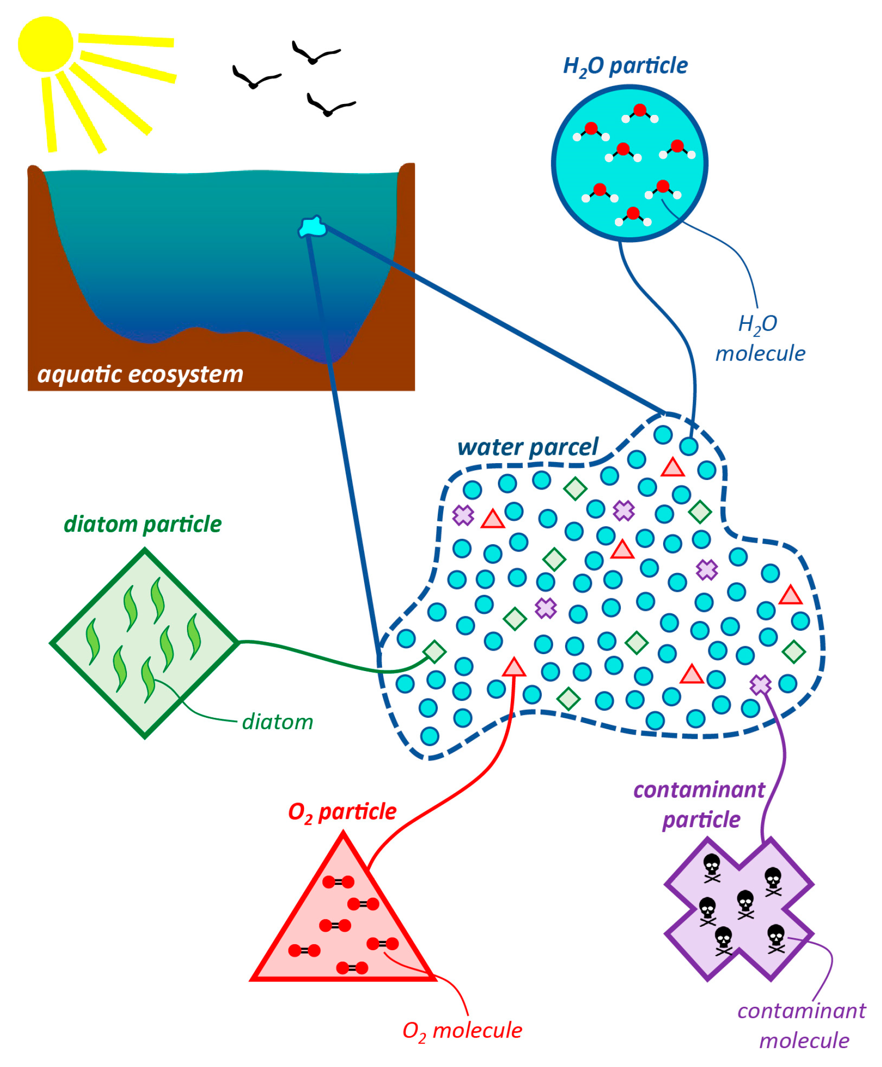
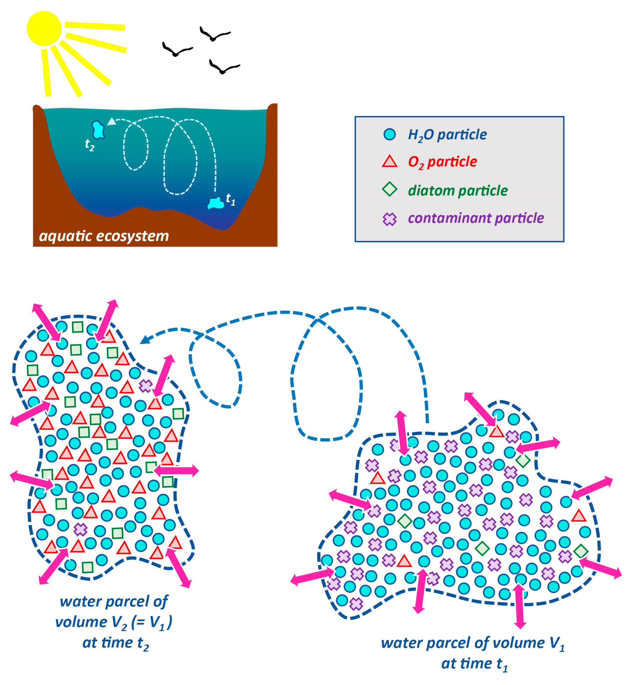
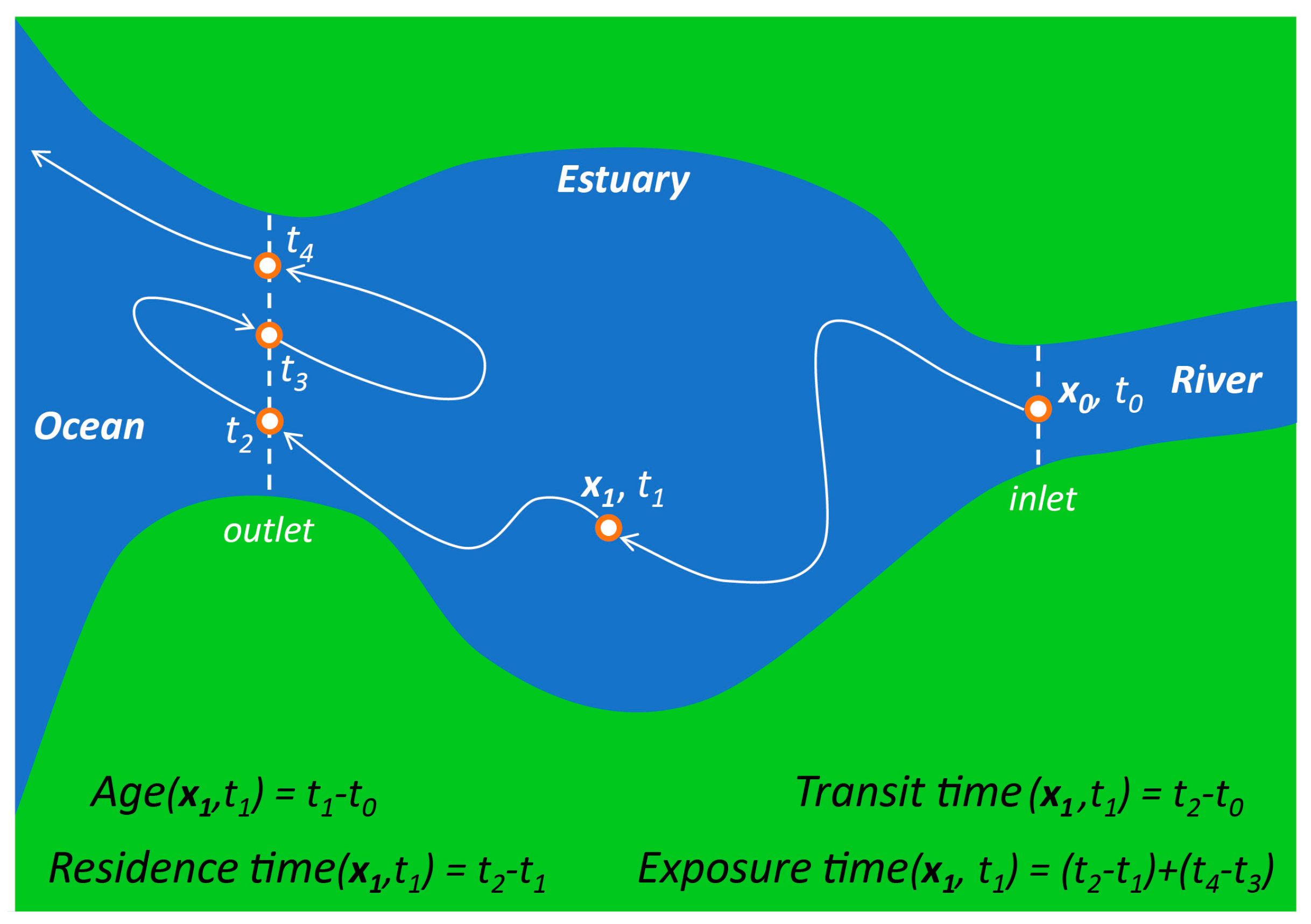
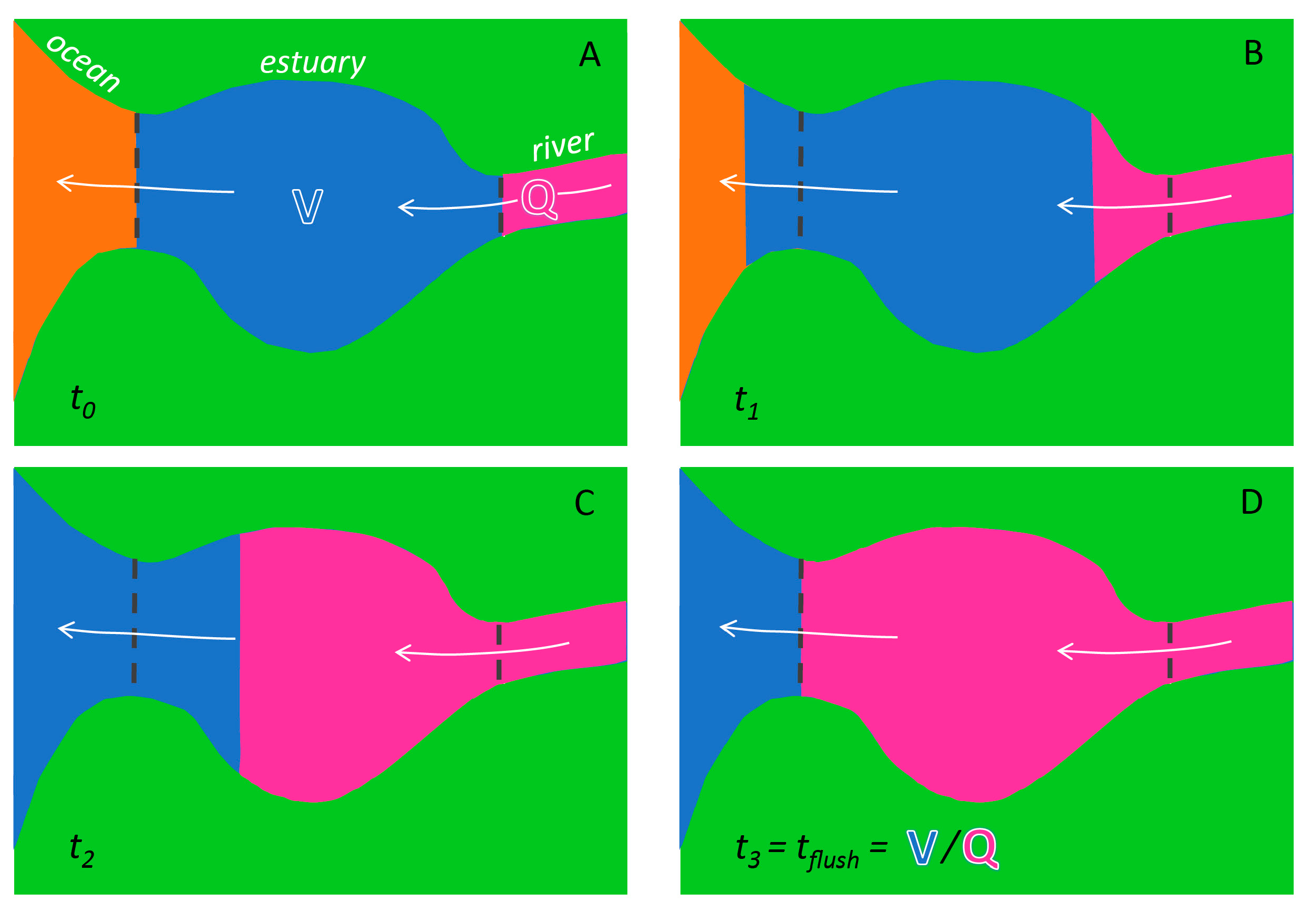
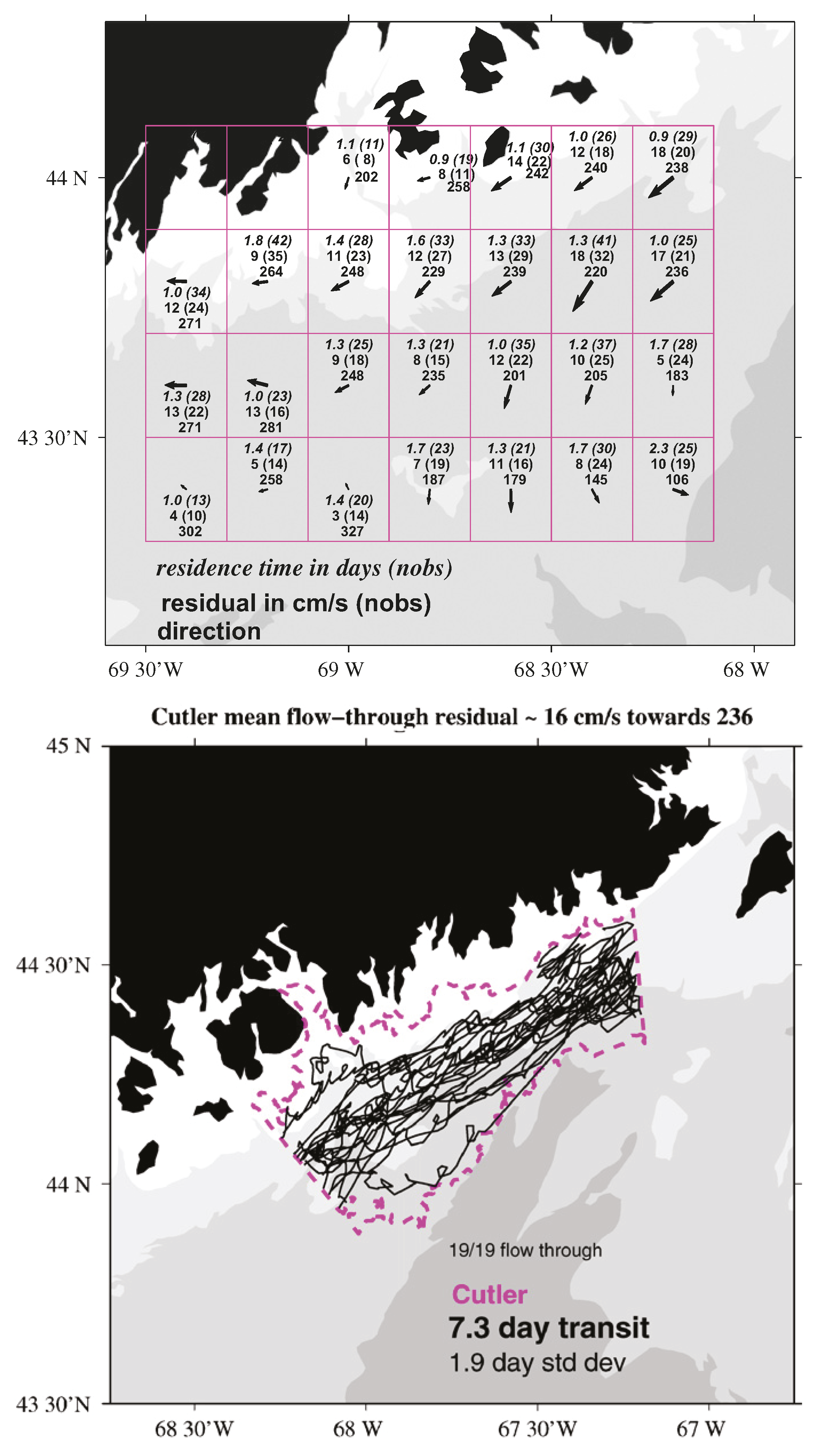
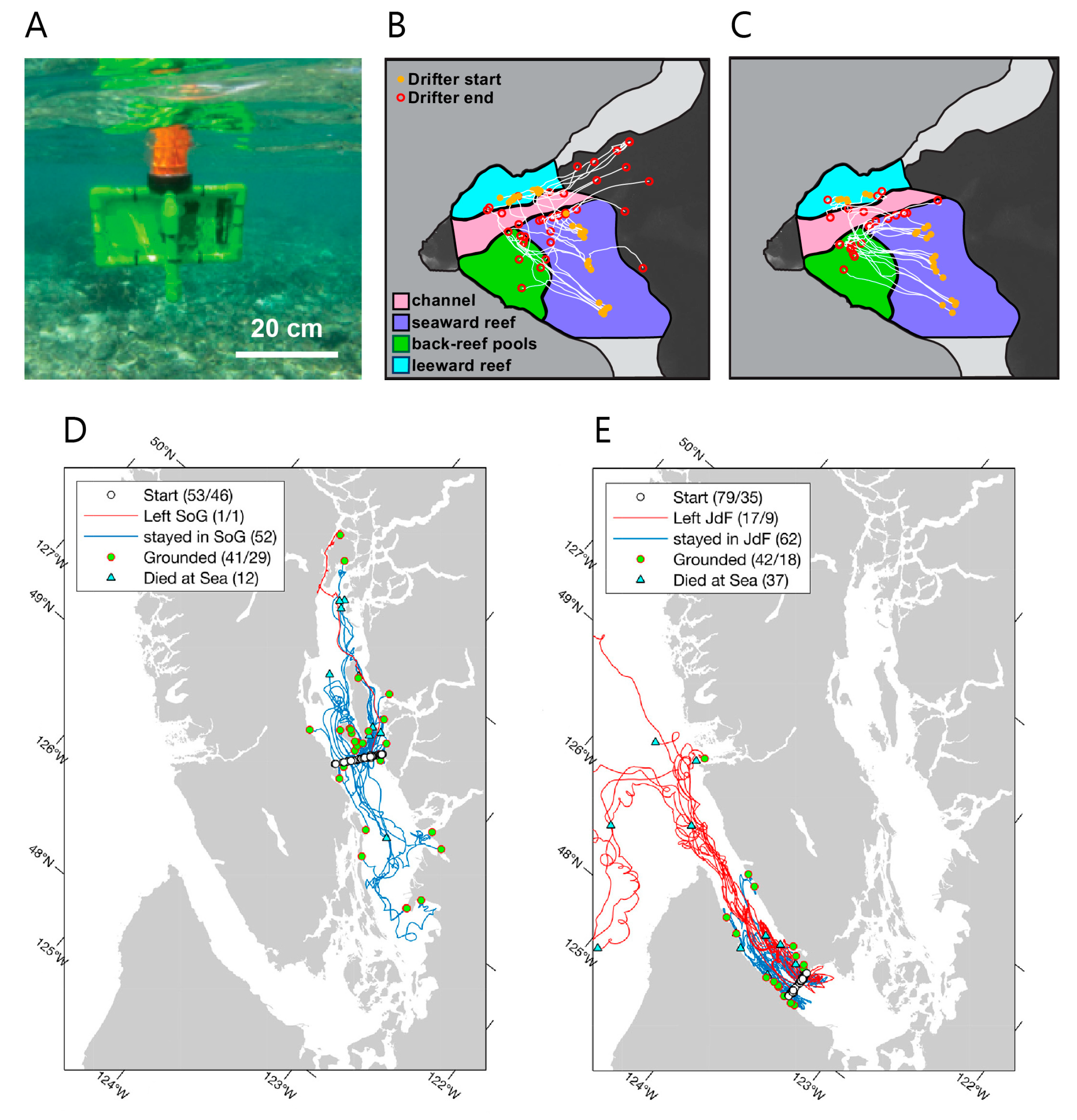
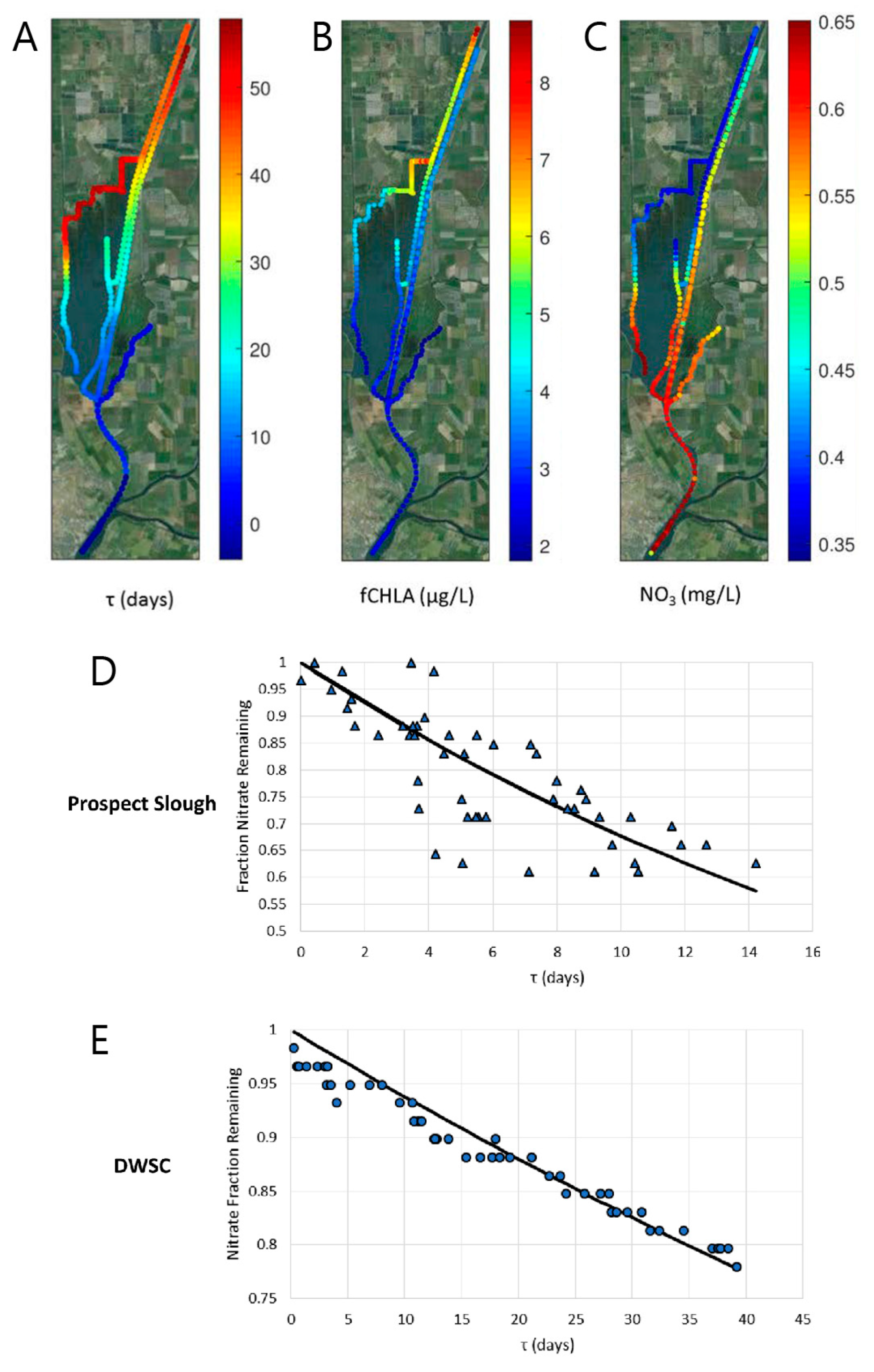
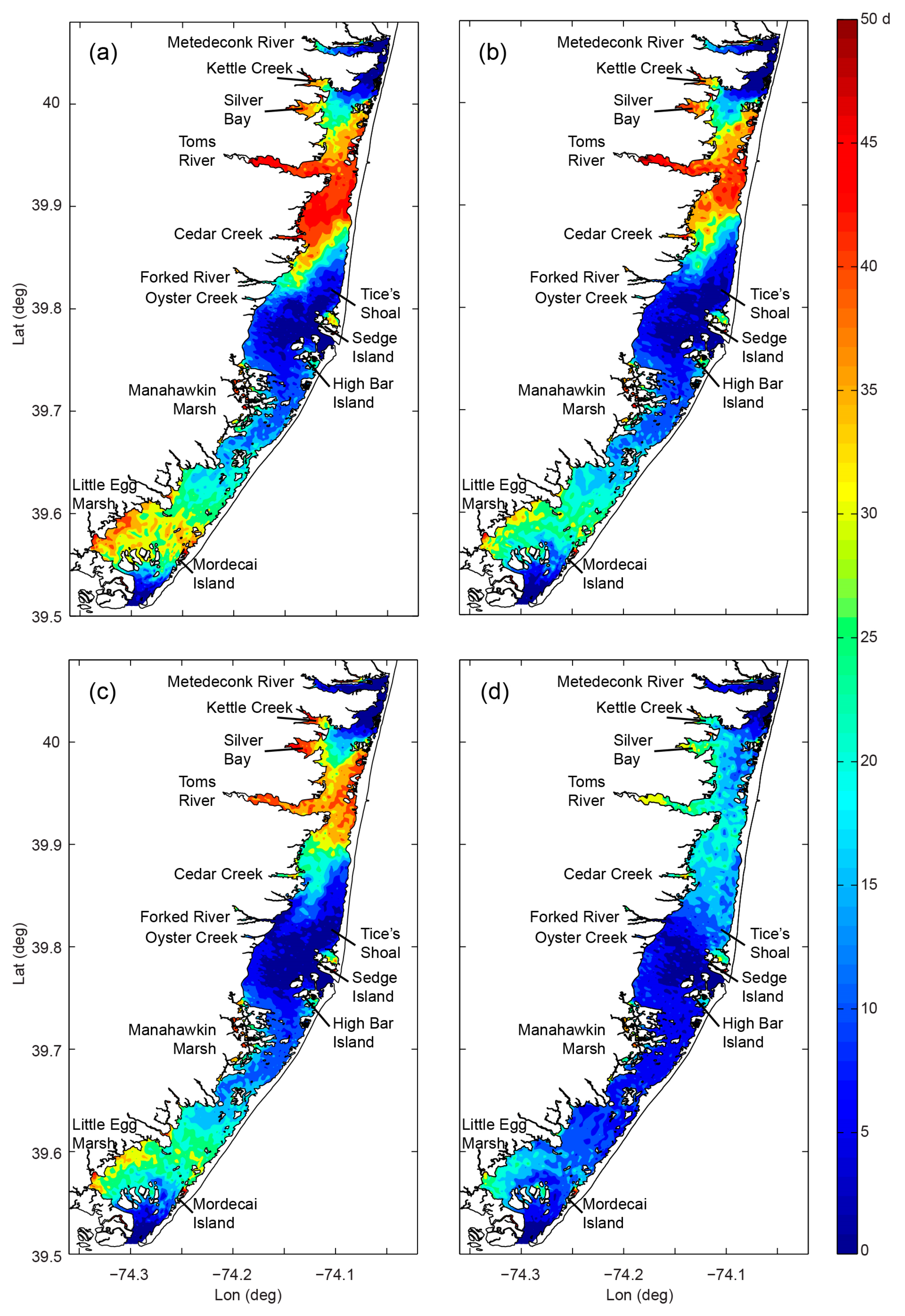
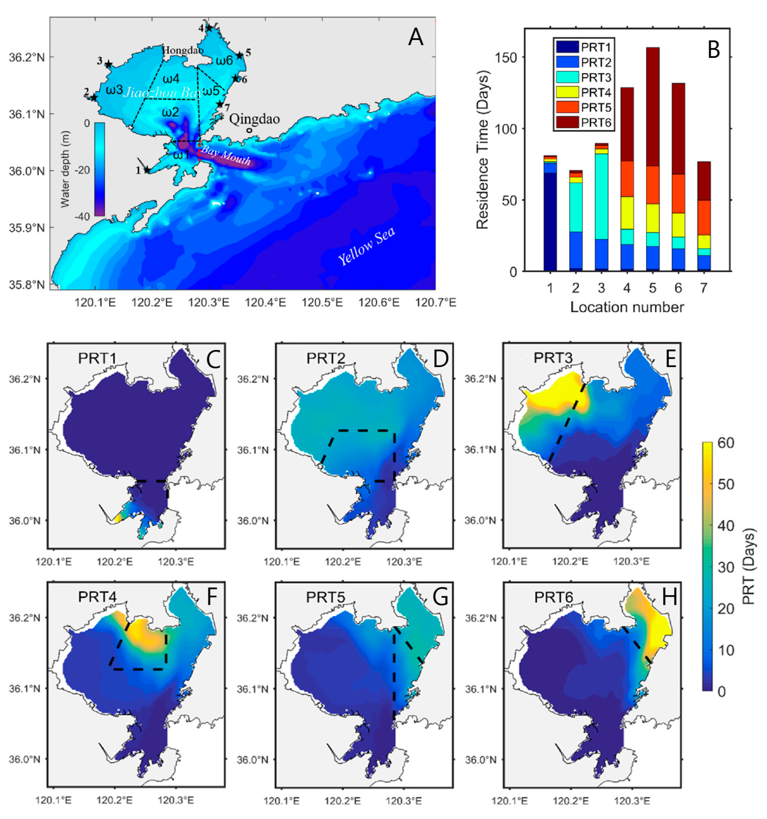
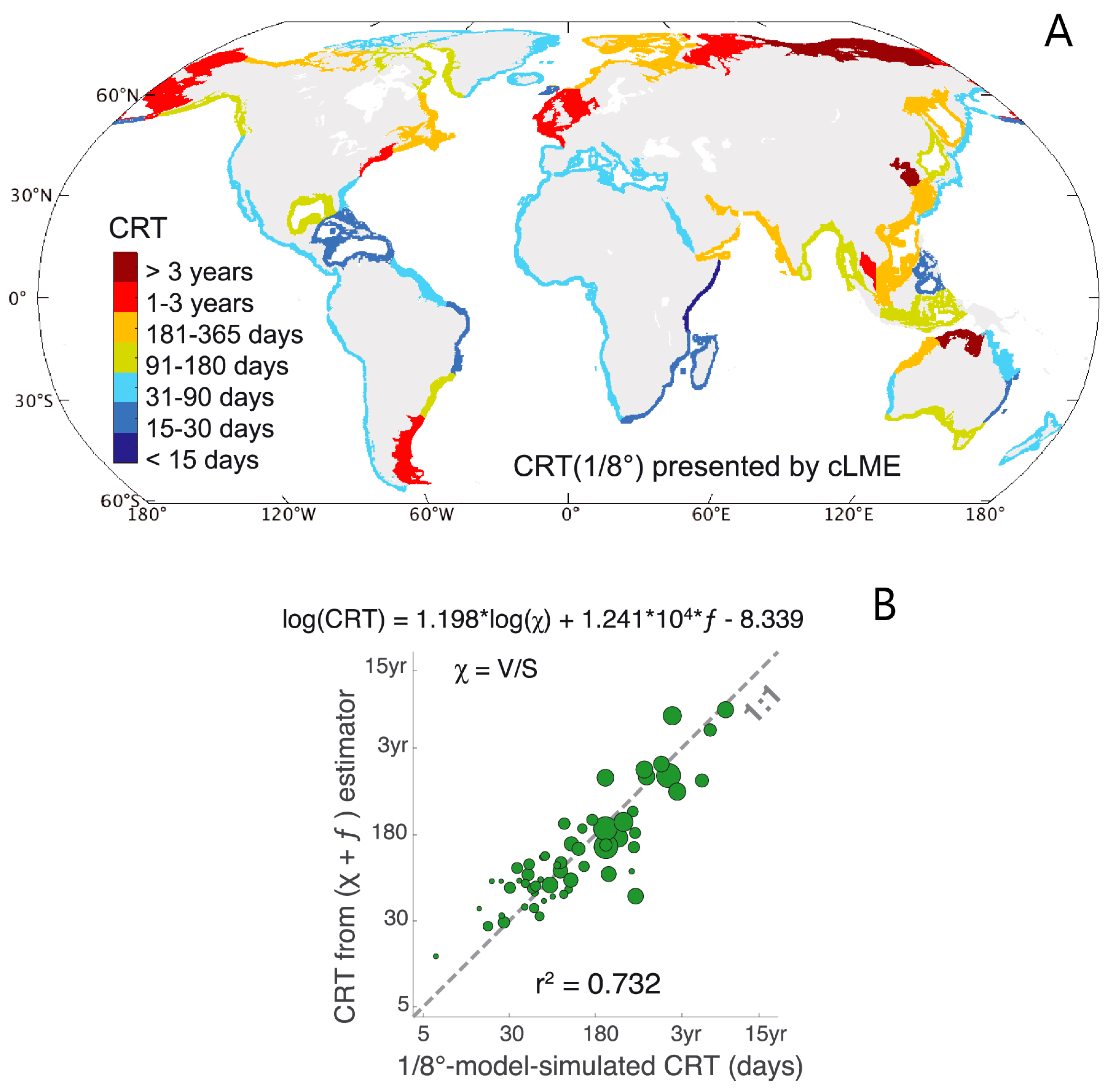
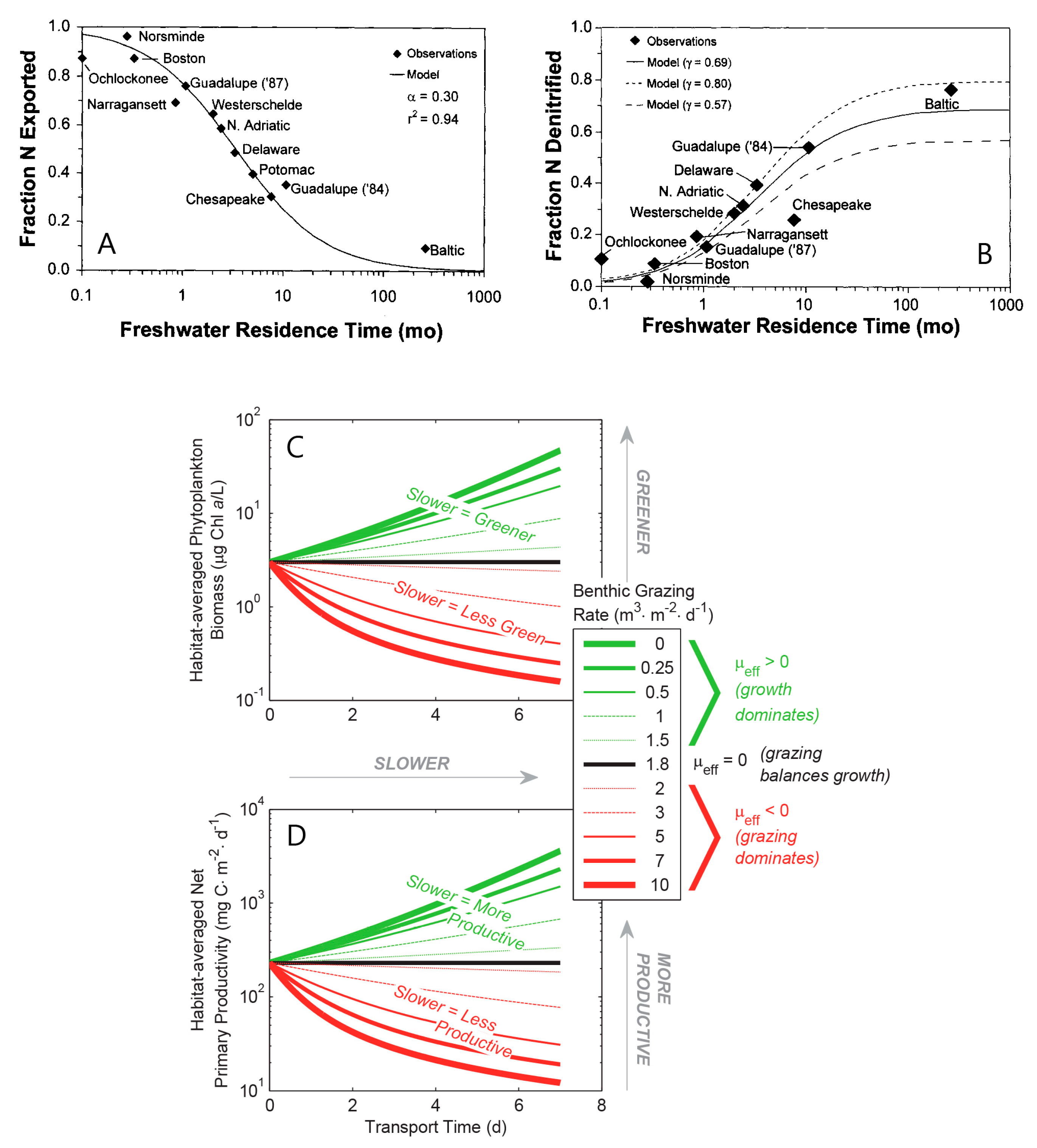
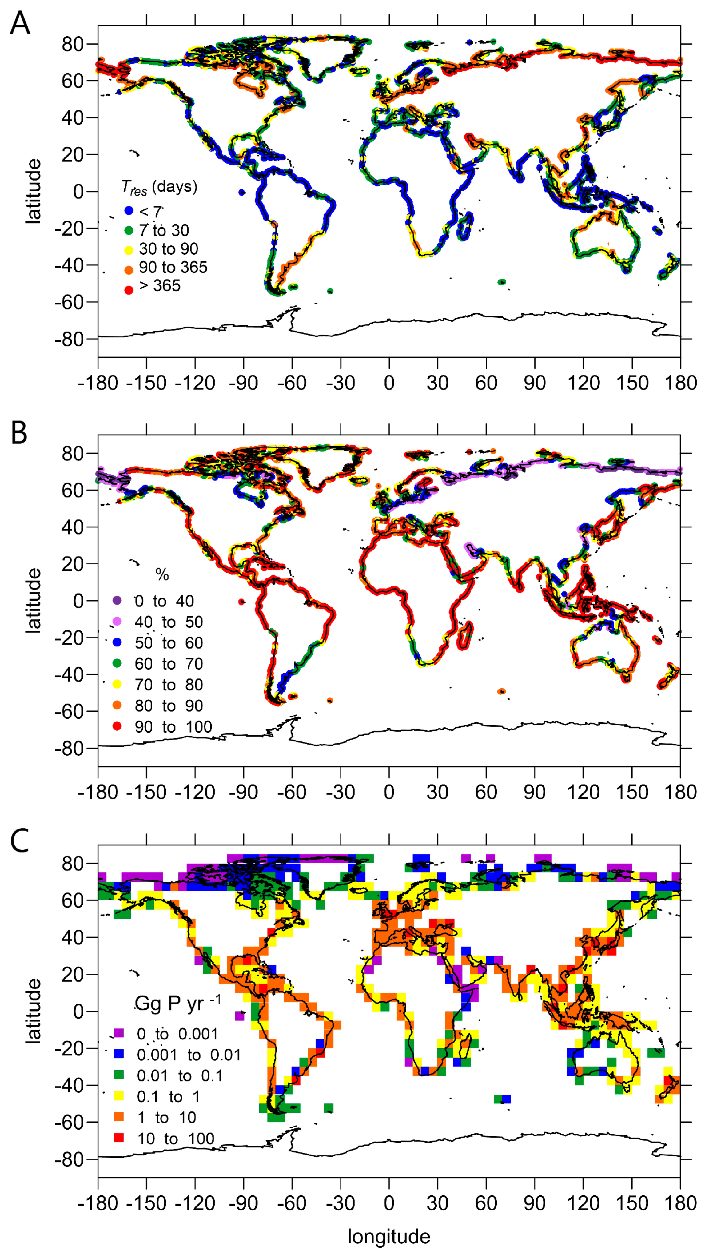
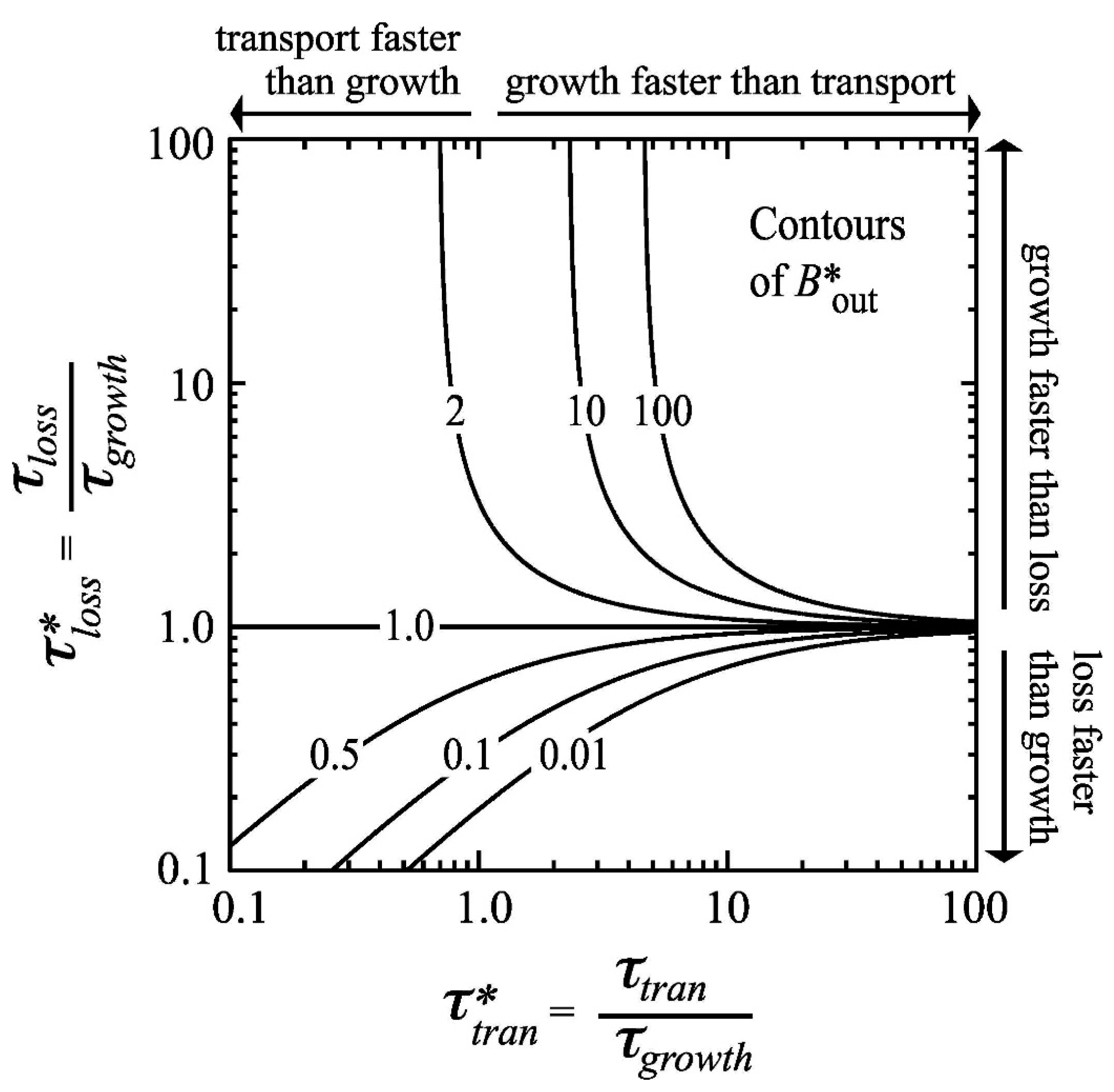
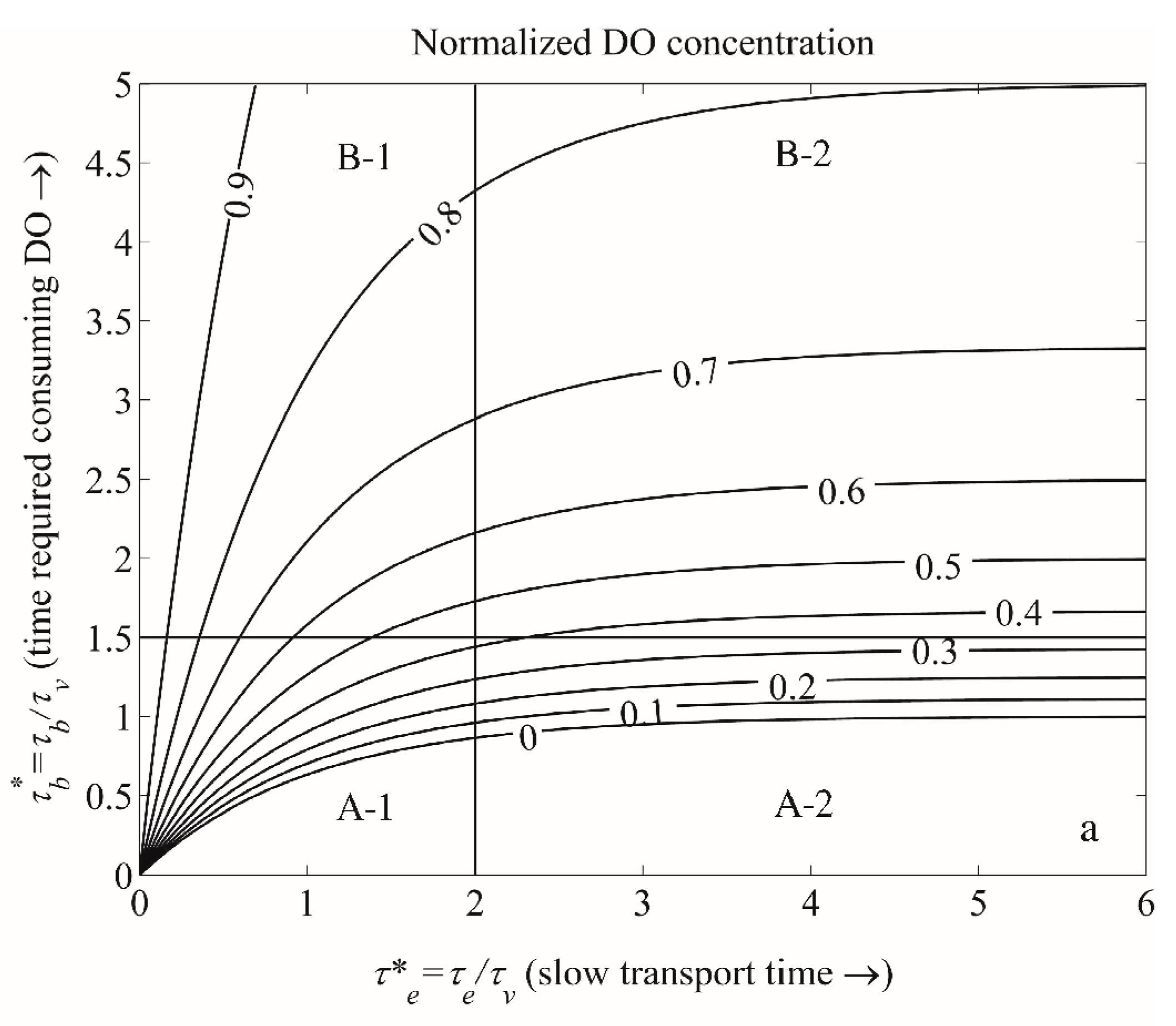
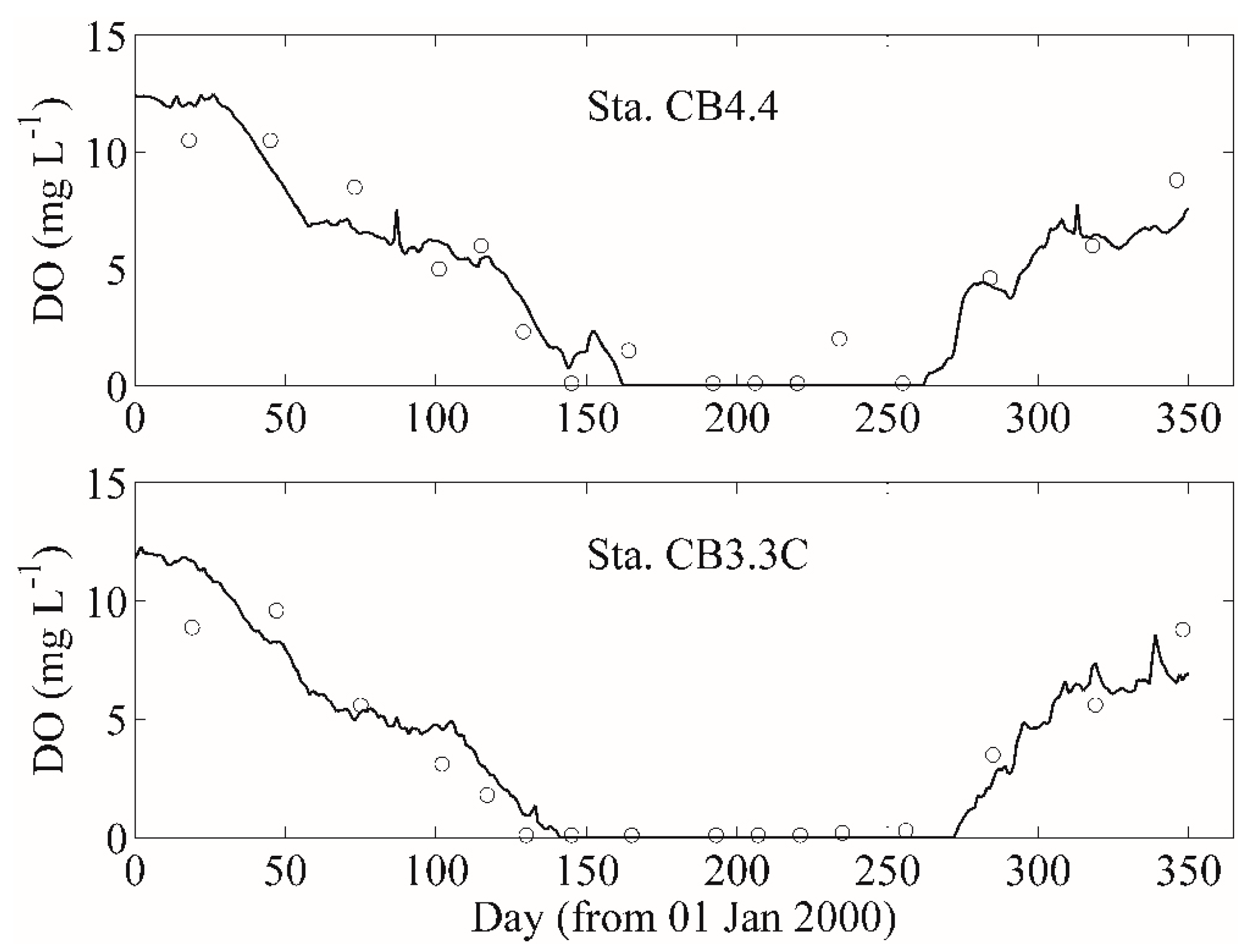
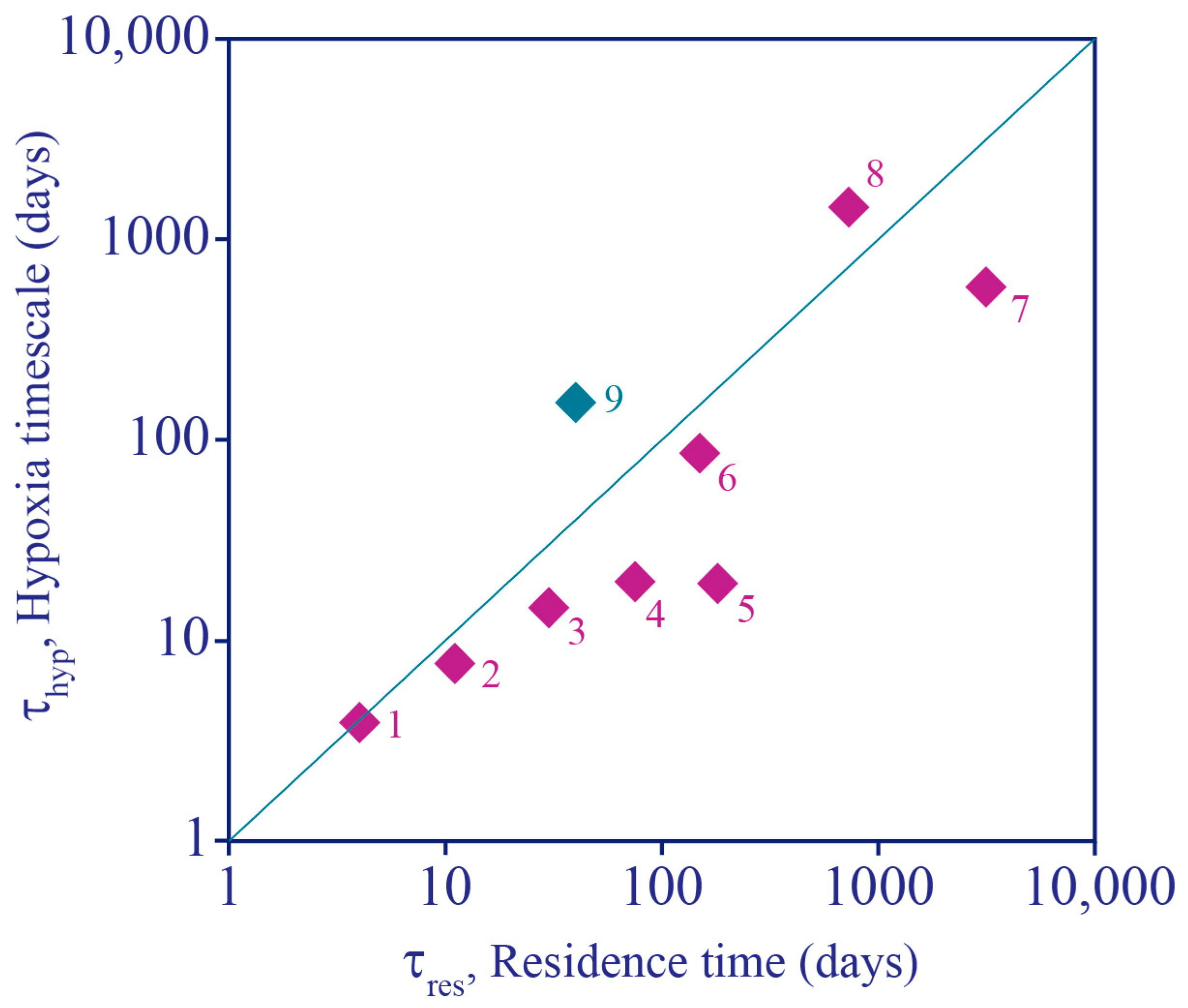
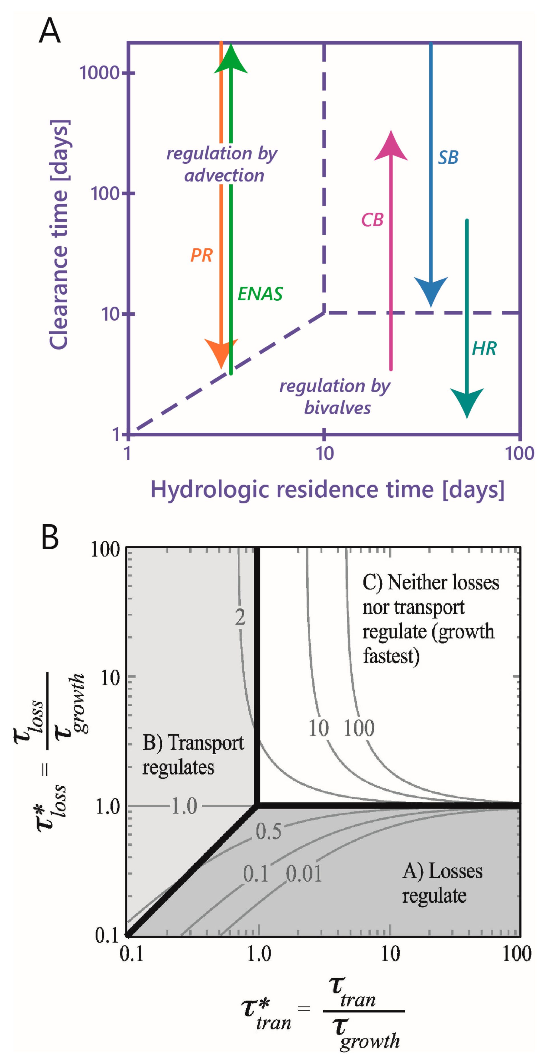
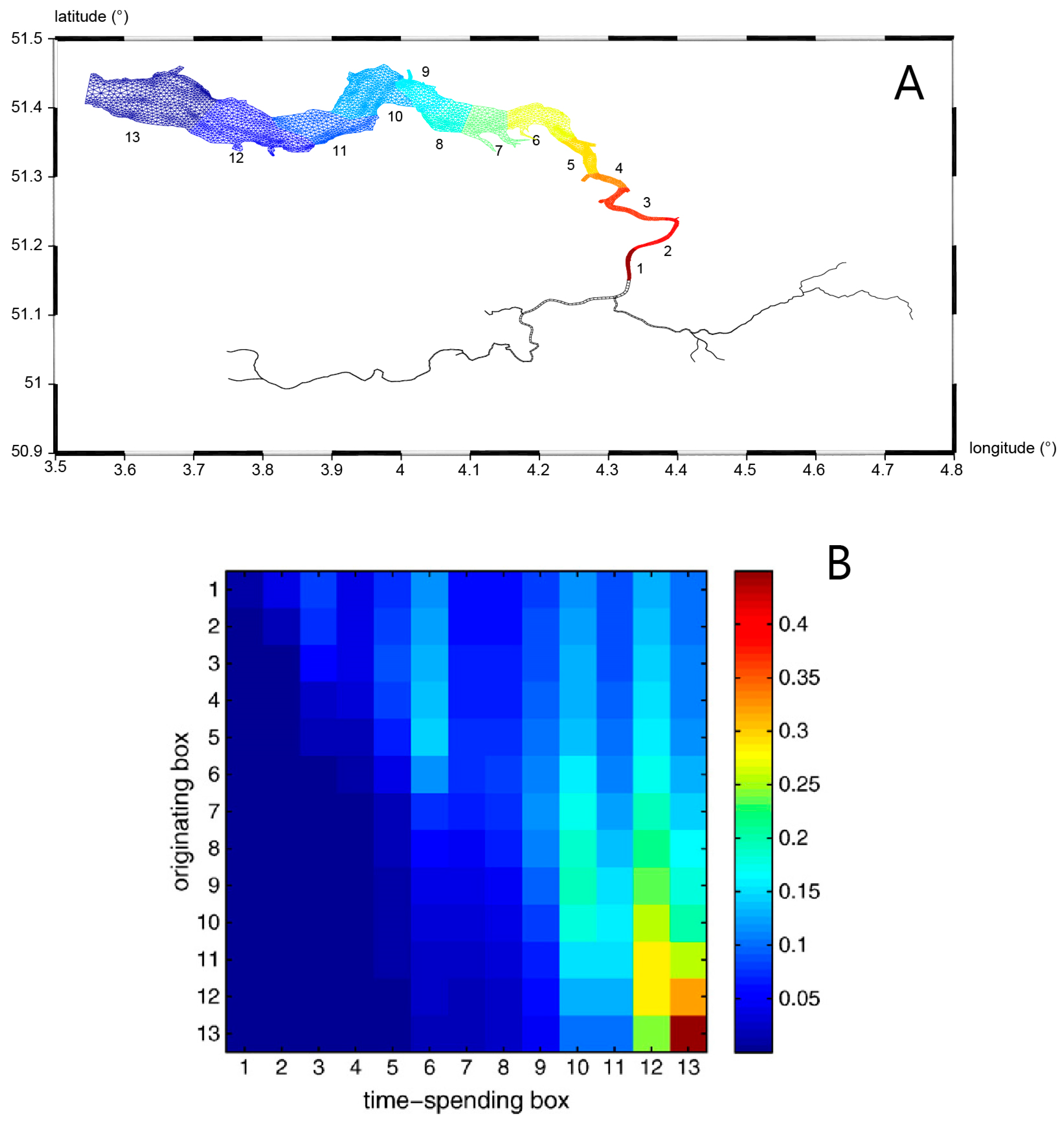
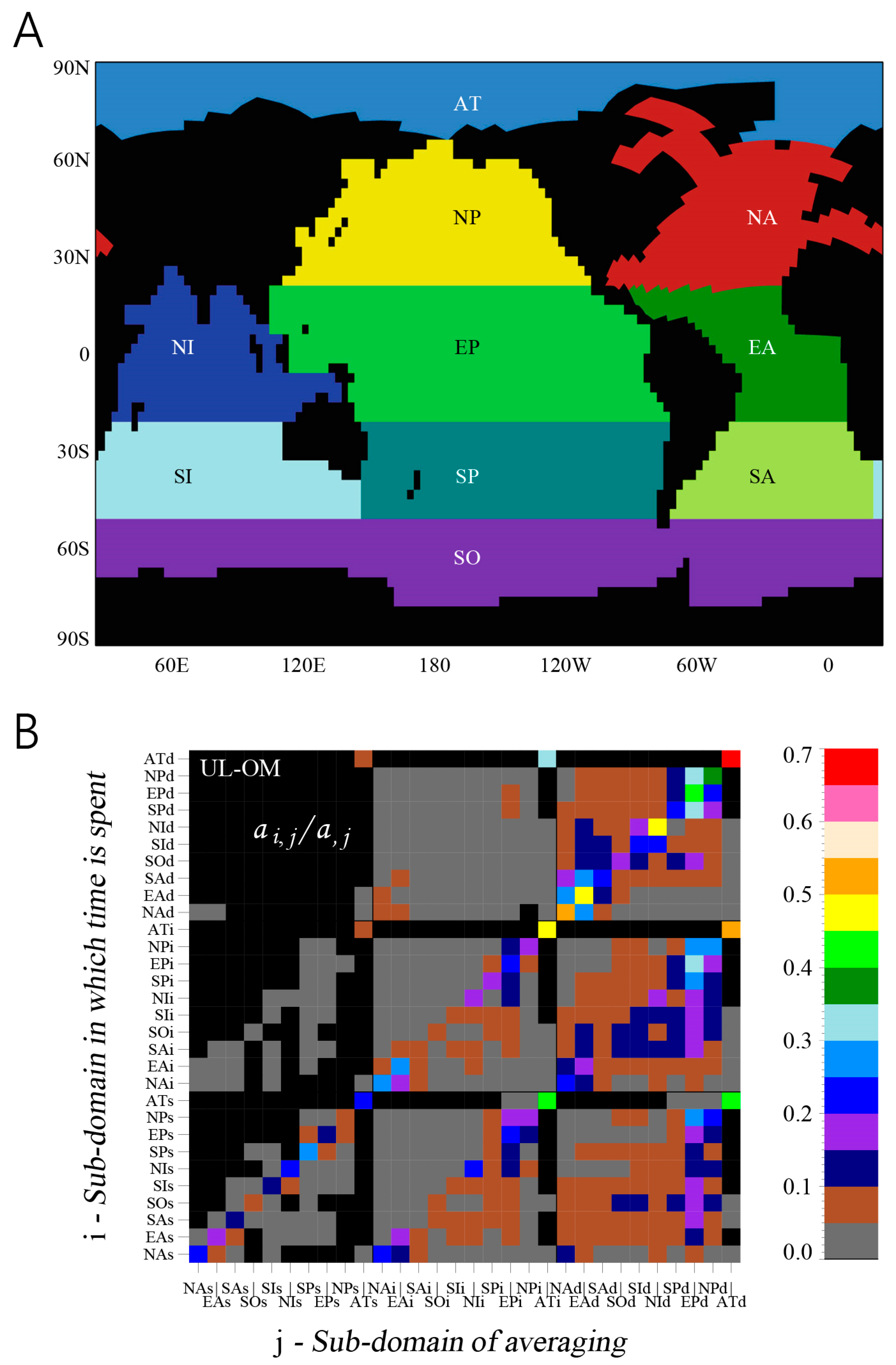
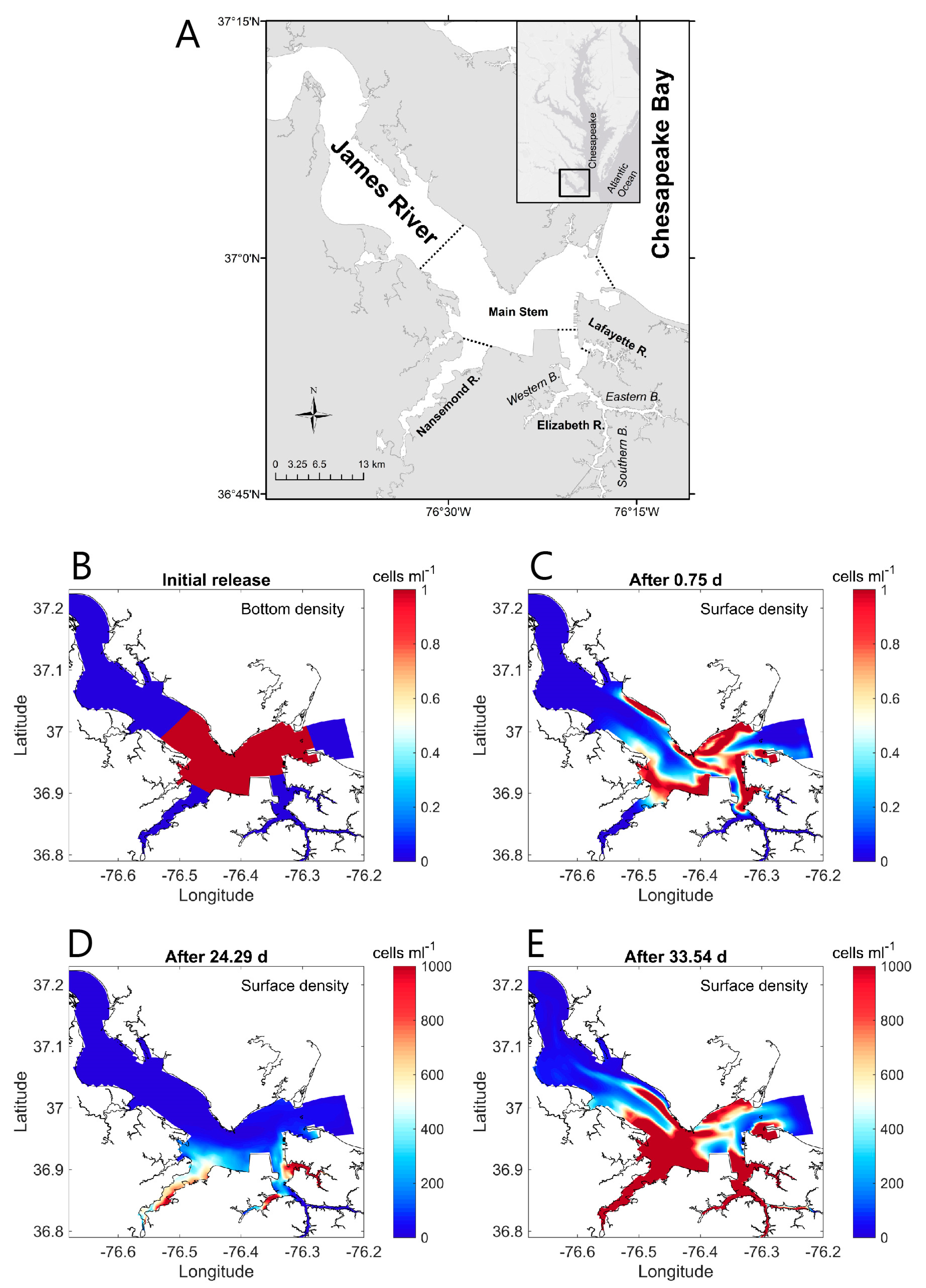
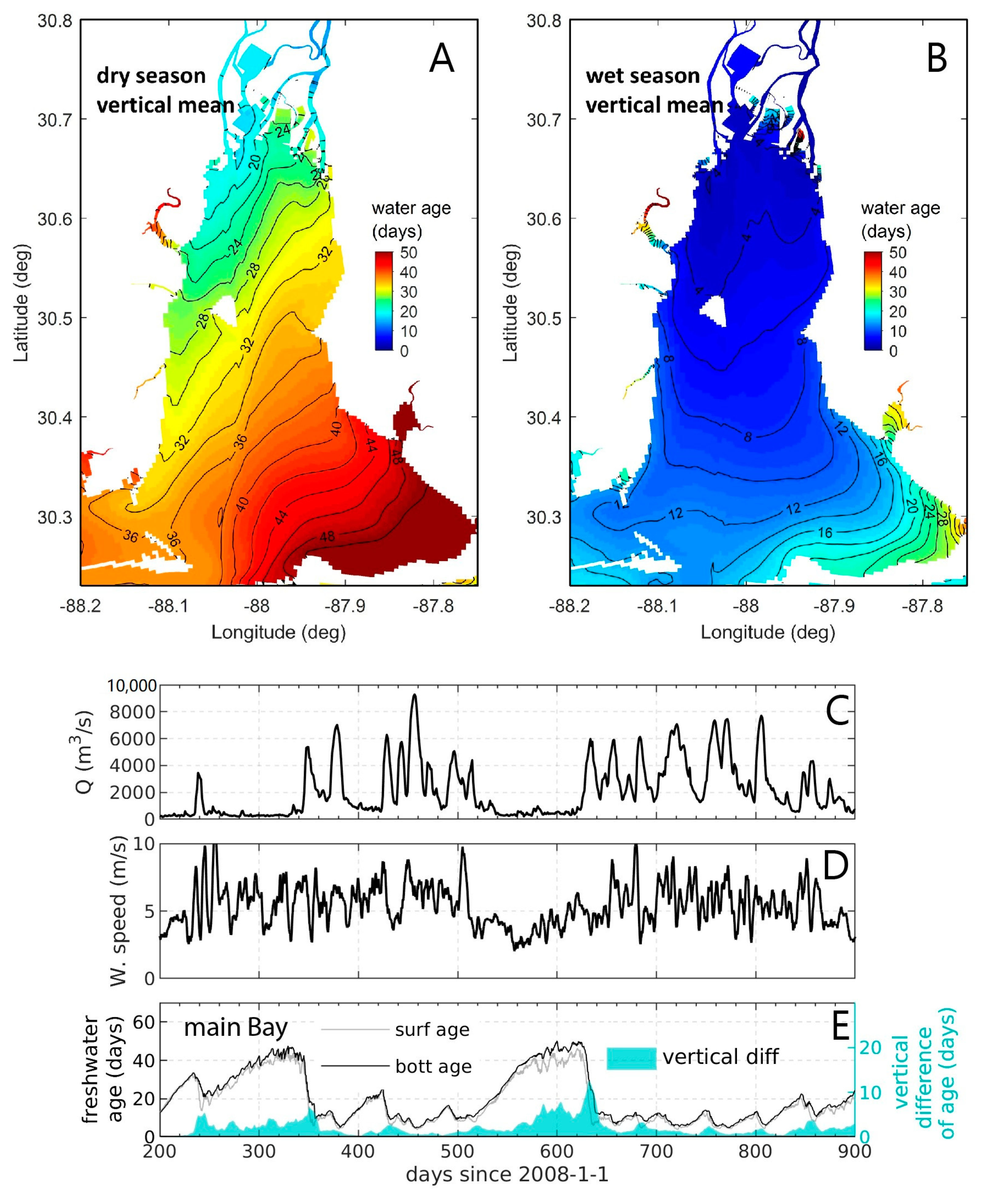
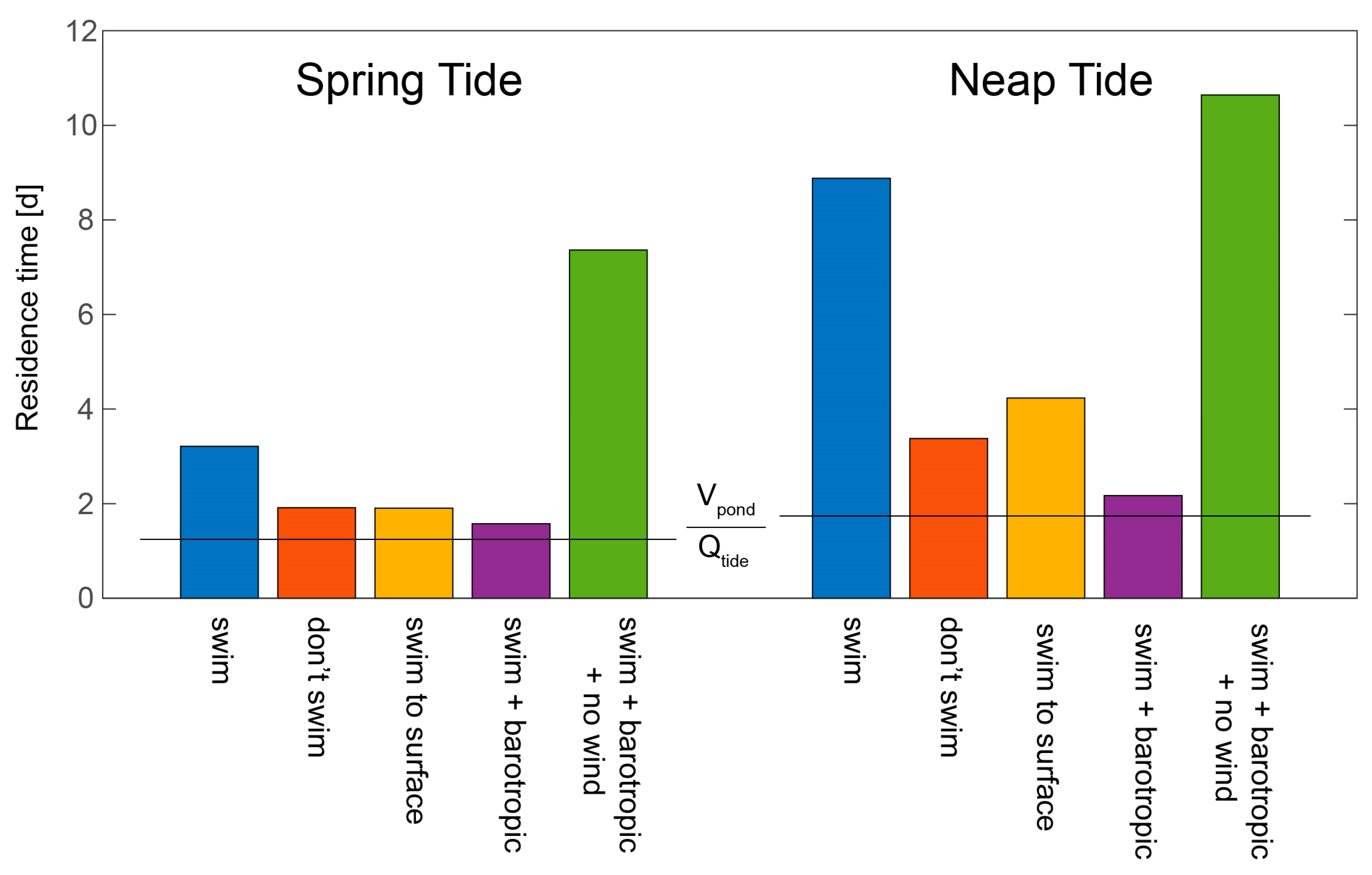
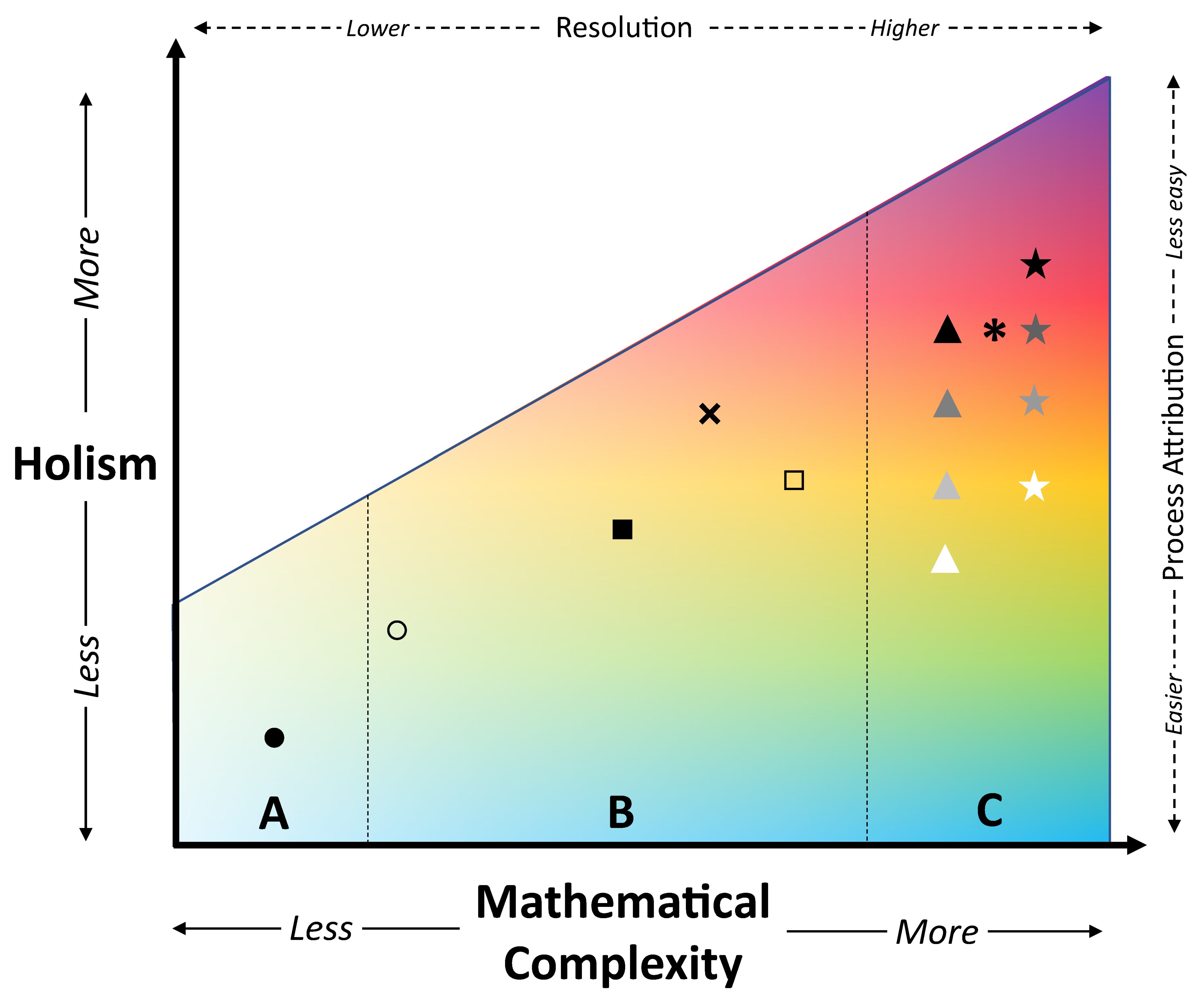
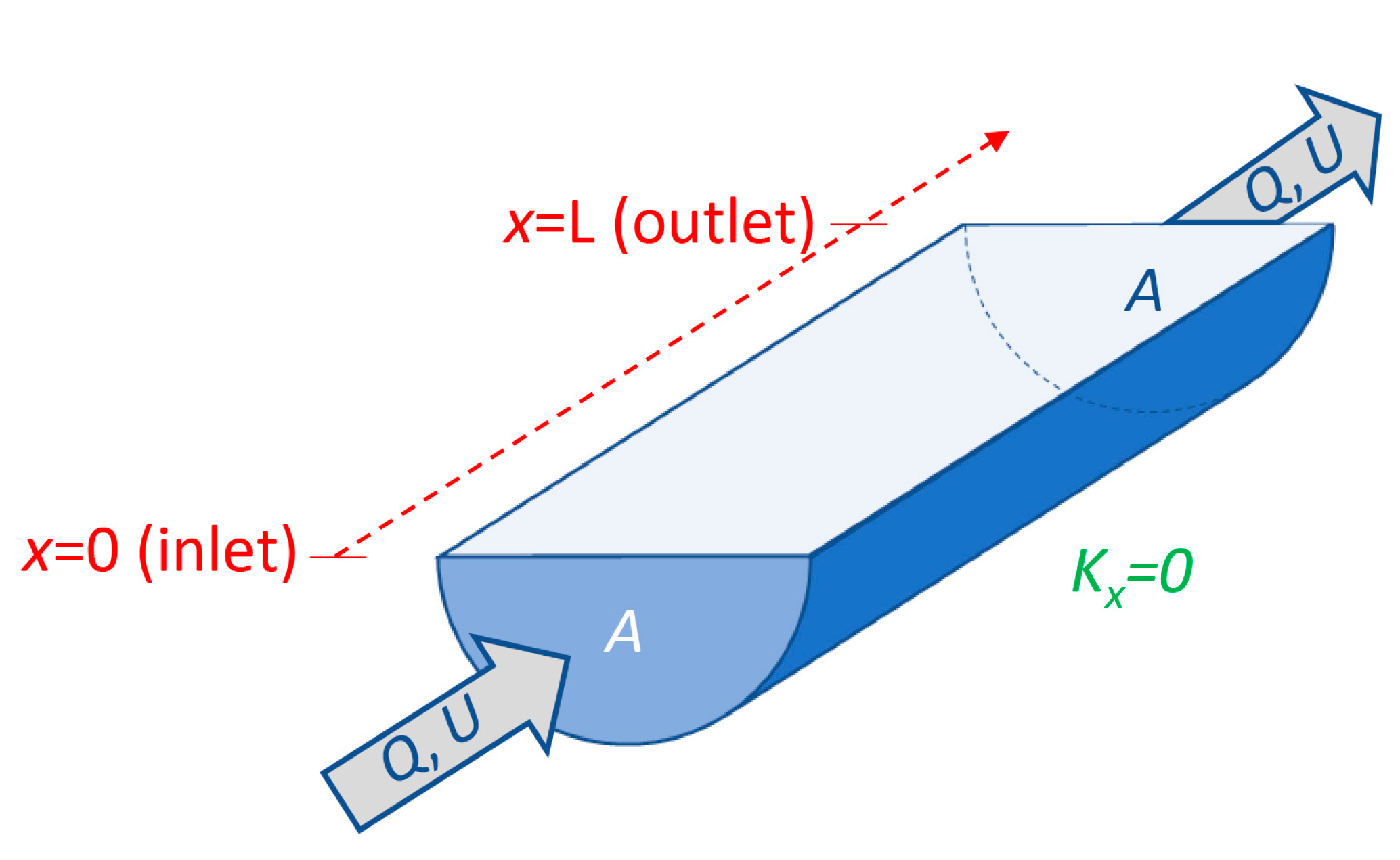
Figure 1. Cartoon depicting the relationships between water parcels, particles, and molecules, cells, etc., as defined herein. A water parcel is a mixture of particles, the most numerous of which are pure water particles. A particle is a material point at which many atoms, molecules, cells, etc., of an individual constituent or aggregate are concentrated. (Following Deleersnijder et al. [63]).
Water 12 02717 g001
Figure 2. Cartoon depicting a water parcel as it is transported through an aquatic ecosystem between times t1 and t2. The water parcel’s volume is constant, but its shape is not. Due to diffusion (magenta arrows), the particles contained within the parcel at t2 are not the same as the particles contained in the parcel at t1. Each “particle” is composed of multiple molecules, atoms, or cells of a particular constituent or aggregate. (Following Deleersnijder et al. [63]).
Water 12 02717 g002
Figure 3. Schematic depicting the relationships between space- and time-dependent age, (strict) residence time, transit time, and exposure time, following Zimmerman [96], Delhez [98], Shen and Haas [121], Viero and Defina [130], Andutta et al. [22], and others. The dots represent successive locations for a single particle following a trajectory passing through locations xi at times ti. x0 and t0 are the initial location and time.
Water 12 02717 g003
Figure 4. Simplified depiction of advective, river-driven estuarine flushing, idealized as plug flow (perfect mixing over the flow cross section, zero mixing in the streamwise direction). Panels (AD) follow a progression through time of river water gradually replacing estuarine water initially present at time t0. V is estuarine volume, and Q is river discharge. River water is depicted as magenta; original estuarine water is blue; water outside the estuary mouth is orange. Gray dashed lines represent upstream and downstream boundaries of the estuary.
Water 12 02717 g004
Figure 5. Based on a series of 45-day numerical particle transport simulations of Galveston Bay (TX, USA) by Rayson et al. [100]: (a) e-folding flushing times for particles initialized on each day for a period spanning mid-March to mid-July 2009. Triangles represent start times for simulations used for exponential fits shown in (b), with the blue triangle representing a high discharge period and the red triangle representing a low discharge period. (b) Example exponential fits for particle -tracking simulations with the three different start times indicated by the triangles in (a). Blue (red) dots and and dashed lines represent the model output and curve fit, respectively, for high (low) discharge periods. (c) RMSE (root mean square error) of the exponential best fit for all times modeled. (Reproduced with permission from M. Rayson, Journal of Geophysical Research: Oceans; published by Wiley, 2016.).
Water 12 02717 g005
Figure 6. Simplified depiction of the e-folding flushing time, driven by river, tidal, and/or other flushing processes. Panels (AD) follow a progression through time of C, the estuarine concentration of a tracer or other constituent. The e-folding mathematical construct is based on the assumption of perfect mixing within the water body of interest (in this case, the estuary). Dark gray dashed lines represent upstream and downstream boundaries of the estuary. Dark purple represents initial estuarine water. Light gray represents replacement water.
Water 12 02717 g006
Figure 7. Results from the drifter field studies of Manning et al. [103] in the Gulf of Maine. Upper Panel: calculated residence times in days (italics), low frequency speed in cm/s, and direction in degrees True. Number of observations (“nobs”) is in parentheses. Lower Panel: tracks of drifters entering waters offshore Cutler Maine from the northeast and heading southwest in the Eastern Maine Coastal Current. Transit time (7.3 d) is the mean time for drifters to traverse the region outlined in purple. (Modified from Manning et al. [103], with permission from Elsevier).
Water 12 02717 g007
Figure 8. From the drifter studies of Storlazzi et al. [102] in Faga’alu Bay (American Samoa): (A) a deployed drifter; individual drifter tracks, with orange symbols representing drifter deployment locations and red circles representing drifter recovery locations for conditions of (B) calm and (C) strong winds. (Modified from Storlazzi et al. [102].) From the drifter field studies of Pawlowicz et al. [104]: tracks for drifters released in (D) the northern Strait of Georgia (SoG) and (E) Victoria Sill in the Salish Sea. Statistics in legends represent the number of tracks for each category; when two numbers are provided separated by a slash, the first is number of tracks, and the second is the number of unique drifter IDs [104]. “JdF” is “Juan de Fuca” Strait. (Modified from Pawlowicz et al. [104] and licensed under CC BY 4.0 (https://creativecommons.org/licenses/by/4.0/)).
Water 12 02717 g008
Figure 9. (A) Water age “τ”, (B) chlorophyll a fluorescence, and (C) nitrate, based on concurrent mapping by Downing et al. [173] aboard a high-speed boat in the Cache Slough Complex of the Sacramento-San Joaquin Delta (USA). Low (high) fCHLA generally corresponded with small (large) τ. Nitrate had roughly the opposite pattern relative to τ. For (D) Prospect Slough and (E) the Sacramento Deep Water Ship Channel (“DWSC”), fits to an exponential relationship between change-in-nitrate versus change-in-water-age along boat tracks, used to estimate total-ecosystem net nitrate uptake rate. Estimated uptake rates were 0.039 d−1 in Prospect Slough and 0.006 d−1 in the DWSC. (Adapted from Downing et al. [173] (https://pubs.acs.org/doi/10.1021/acs.est.6b05745), with permission from American Chemical Society. This is an unofficial adaptation of an article that appeared in an ACS publication. ACS has not endorsed the content of this adaptation or the context of its use. Further permissions related to the material excerpted should be directed to the ACS).
Water 12 02717 g009
Figure 10. Spatially variable residence times computed by Defne and Ganju [101] with coupled 3D hydrodynamic and particle tracking models applied to Barnegat Bay-Little Egg Harbor (NJ, USA). The scenarios shown are (a) tidal forcing only, (b) tidal plus remote coastal forcing, (c) like (b) but with river flow added, (d) like (c) but with meteorological forcing added. Two inlets—Little Egg Inlet at the southern end and Barnegat Inlet near the center—connect the ocean and estuary (see Figure 1 in [101] for detailed site map). (Modified from Defne and Ganju [101]).
Water 12 02717 g010
Figure 11. Lin and Liu’s [141] (A) bathymetry map of Jiaozhou Bay (China), showing six subregions (ω1ω6) in which partial residence times (PRTs) were calculated in (BH), and seven release points (stars) for which PRTs in the subregions are shown in (B). (B) For particles initiated at each of seven locations, PRTs shown are time spent in each of six subregions before leaving the bay. For a given release location, the sum of the PRTs equals the total residence time within Jiaozhou Bay. (CH) Spatial maps for each subregion representing time spent in the subregion for particles initiated at every location in the domain. Dashed lines represent the boundaries of each subregion. (Adapted by permission from Springer Nature Customer Service Center GmbH: Springer Nature, Ocean Dynamics, Partial residence times: determining residence time composition in different subregions, Lin and Liu, 2019. https://www.springer.com/journal/10236).
Water 12 02717 g011
Figure 12. (A) A global map of coastal residence times (CRTs) simulated by Liu et al. [207] using high-resolution, coupled global ocean-ice models and a novel variation on an age tracer approach; (B) simple model of CRT as a function of Coriolis parameter f and a geometric parameter χ, which is the ratio of total coastal system volume to total open boundary area. (Modified with permission from Xiao Liu, Geophysical Research Letters; published by Wiley, 2019).
Water 12 02717 g012
Figure 13. Dettmann’s [214] simple models for fraction of upland nitrogen loading to an estuary that is (A) exported (Equation (2) herein) and (B) denitrified (Equation (3) herein), expressed as functions of “freshwater residence time” and fit to data for several estuaries. “γ” in Dettmann’s [214] denitrification plot (B) is referred to as “ε” in Equation (3) and the text herein. (Modified from Dettmann [214].) Calculations of habitat-averaged phytoplankton (C) biomass and (D) productivity based on Lucas and Thompson’s [215] simple models expressed as a function of transport time (Equation (4) herein for algal biomass). (Modified from Lucas and Thompson [215]).
Water 12 02717 g013
Figure 14. Based on the global scale, simple mathematical modeling of Sharples et al. [210]: (A) average residence time “Tres” on the continental shelf; (B) estimated proportion of riverine DIP (dissolved inorganic phosphorus) exported to the open ocean; (C) estimated annual DIP mass export to the open ocean. The authors performed the same calculations for dissolved inorganic nitrogen and provided uncertainty estimates (not shown here). (Modified with permission from J. Sharples, Global Biogeochemical Cycles; published by Wiley, 2017).
Water 12 02717 g014
Figure 15. Contours of B o u t , the ratio of outgoing algal biomass concentration to incoming concentration, as a function of two dimensionless parameters, τ l o s s (the ratio of the algal loss timescale to the growth timescale) and τ t r a n (the ratio of the transport timescale to the algal growth timescale). Based on the simple, timescale-based mathematical model of [23], Equation (7) herein. (From Lucas et al. [23]).
Water 12 02717 g015
Figure 16. Contours of c:cs (ratio of bottom layer dissolved oxygen concentration (DO) to surface layer DO), as a function of two dimensionless parameters, τ b (the biochemical consumption timescale normalized by the vertical exchange timescale) and τ e (the timescale for transport driven by gravitational circulation normalized by the vertical exchange timescale). Based on the simple, timescale-based mathematical model of Shen et al. [21] (Equation (8) herein). Rectangular regions delineate regimes associated with control of DO by particular processes and/or likelihood of hypoxia. (Reuse and minor adaptation from Shen et al. [21], with permission from Wiley. © 2013, by the Association for the Sciences of Limnology and Oceanography, Inc.)
Water 12 02717 g016
Figure 17. Comparisons of the simple Shen et al. [21] model (solid lines) and DO observations at two stations in the Chesapeake Bay. (Reuse and minor adaptation from Shen et al. [21], with permission from Wiley. © 2013, by the Association for the Sciences of Limnology and Oceanography, Inc.).
Water 12 02717 g017
Figure 18. Hypoxia timescale versus residence time for several hypoxic estuarine and shelf systems, as estimated by Fennel and Testa [132]. Systems falling below the diagonal 1:1 line are consistent with the authors’ hypothesis that γ, the ratio of the hypoxia timescale to the residence time, is less than unity for hypoxia to occur. Systems analyzed: (1) Pearl River Estuary (China); (2) East China Sea; (3) Northern Gulf of Mexico; (4) Long Island Sound (USA); (5) Chesapeake Bay (USA); (6) Northwestern Black Sea; (7) Baltic Sea; (8) Gulf of St. Lawrence (Canada); (9) Namibian Shelf. (Redrawn from Fennel and Testa [132] with the permission of K. Fennel.)
Water 12 02717 g018
Figure 19. (A) The conceptual model of Strayer et al. [232], which extended that of Dame [233] and described three domains of control of phytoplankton (i.e., by advection, bivalve grazing, or phytoplankton growth). Strayer et al. [232] explained that domain boundaries may be different from those shown, depending on phytoplankton net growth rates. Arrows describe how bivalve clearance times in five estuarine, river, and stream ecosystems changed over time as a result of bivalve invasion or population decline. Ecosystems are the following: HR, the Hudson River (NY, USA) after the Dreissena polymorpha (zebra mussel) invasion; SB, Suisun Bay (CA, USA) after invasion by Potamocorbula amurensis; CB, the Chesapeake Bay (USA) after the decline of oyster populations; ENAS, a typical eastern North American stream after unionid decline; and PR, the freshwater tidal Potomac River (MD, USA) after the Corbicula fluminea invasion. (Redrawn from Strayer et al. [232] with the permission of D. Strayer.) (B) Reprise of Figure 15 with shaded areas added to describe domains of control on phytoplankton biomass [23], extending the conceptual model of Strayer et al. [232] in panel (A). Contours represent values of B o u t , the ratio of outgoing algal biomass concentration to incoming concentration. (From Lucas et al. [23].)
Water 12 02717 g019
Figure 20. (A) Zoom-in of the computational mesh of De Brauwere et al. [95], showing subregions of the Scheldt Estuary referred to in (B). Subregions were based on the compartmentalization of [235]. (B) Connectivity matrix based on computations of “subdomain exposure times” with a 2D tracer transport model. Colors represent the relative time spent in a particular subregion numbered on the horizontal axis by tracer initialized in a subregion on the vertical axis. (Modified from De Brauwere [95], with permission from Elsevier).
Water 12 02717 g020
Figure 21. (A) Horizontal partitioning of the world ocean by Mouchet et al. [140] for use with a global ocean circulation model to evaluate connectivity between 30 different subdomains (each horizontal partition is split into three boxes in the vertical dimension, denoted by “s” for surface, “i” for intermediate, or “d” for deep in (B)). (B) Connectivity matrix showing computed “partial age” (ai,j) for all subdomains, i.e., the mean time spent by particles in any subdomain i (vertical axis) before reaching the subdomain of interest j (horizontal axis). Partial age is normalized by the mean (total) water age in the corresponding sub-domain. (Adapted by permission from Springer Nature Customer Service Center GmbH: Springer Nature, Ocean Dynamics, Partial ages: diagnosing transport processes by means of multiple clocks, Mouchet et al., 2016. https://www.springer.com/journal/10236).
Water 12 02717 g021
Figure 22. (A) Map of the lower James River (USA) and its tributaries [199]. From a 3D model simulation performed by Qin and Shen [199], algal cell densities (B) specified as the initial condition (non-zero cell densities initially only in the bottom layer of the lower James River mainstem), and computed cell densities (C) after 0.75 d; (D) after 24.29 d, when average surface density of the entire Lafayette River first reached bloom levels (1000 cells/mL); and (E) after 33.54 d, when the average surface density of the mainstem first reached bloom levels. These results are consistent with observations and with a simple theoretical model indicating that a simple parameter—the ratio of subregion residence time to its volume—can predict where harmful algal blooms are first observed [199]. (Modified from Qin and Shen [199], with permission from Elsevier).
Water 12 02717 g022
Figure 23. From Peierls et al. [57], maps of the (A) New River Estuary (NewRE) and (C) Neuse River Estuary (NRE); for the (B) NewRE and (D) NRE, observation based ln(chlorophyll a) versus flushing time estimated with the “date-specific freshwater replacement method” [239]. (Adapted by permission from Springer Nature Customer Service Center GmbH: Springer Nature, Estuaries and Coasts, Non-monotonic Responses of Phytoplankton Biomass Accumulation to Hydrologic Variability: A Comparison of Two Coastal Plain North Carolina Estuaries, Peierls et al., 2012. https://www.springer.com/journal/12237).
Water 12 02717 g023
Figure 24. Maps of computed vertical mean freshwater age in Mobile Bay for (A) the dry season and (B) the wet season, based on the 3D numerical modeling of Du et al. [243]. Timeseries of (C) river discharge, (D) wind speed, and (E) computed freshwater age averaged over the main bay. For the age timeseries, surface water is gray, bottom water is black, and the vertical age difference is cyan [243]. (Modified with permission from J. Du, Journal of Geophysical Research: Oceans; published by Wiley, 2018).
Water 12 02717 g024
Figure 25. Computed residence times for the toxic alga A. fundyense based on the 3D model of Ralston et al. [127] for a pond within the Nauset Estuary (MA, USA). The different bars represent a variety of swimming and forcing cases under spring and neap tide conditions. “Swim”: diel vertical migration up to 1/kw depth, where kw is the light attenuation coefficient. “Don’t swim”: no vertical migration. “Swim to surface”: diel migration to the surface. “Swim + barotropic”: diel vertical migration to 1/kw with barotropic physics (uniform water density and thus no stratification). “Swim + barotropic + no wind”: diel vertical migration to 1/kw with barotropic physics and zero wind forcing. Horizontal lines: the residence time for tidal exchange assuming a well-mixed pond (volume of pond/tidal volume exchange), shown for reference. (Redrawn from Ralston et al. [127] with the permission of D. Ralston).
Water 12 02717 g025
Figure 26. Schematic of diagnostic timescale holism as a function of the mathematical complexity of the calculation method (for computed timescales only). Timescales based on simple algebraic expressions tend to be less holistic, but potentially more useful for purposes of assessing dominant processes (Regime A). Complex numerical models have the potential to produce highly holistic timescales (Regime C) as well as timescale estimates at high spatial and temporal resolution. The effective level of holism depends on the process richness captured by the model simulation. More holistic timescales may be less useful for disentangling the relative speeds (and potential dominance) of individual processes (“process attribution”). Moderately holistic timescales may be derived from moderately complex numerical models or methods (Regime B) or from complex models that exclude some important processes (mid-region of Regime C). Examples: ●—τadv = L/U or τdiff = L2/K. ○— τ r e s ¯ and τ e x p ¯ from Andutta et al. [22], Equations (9) and (10) herein. Timescales derived from the 1D models of Delhez and Deleersnijder [200] or Vallino and Hopkinson [160] ( ); the 2D depth-averaged model of Monsen et al. [87] (□); the 1D hydrodynamic-biological model of Delhez et al. [189] ( × ); the 3D hydrodynamic and transport model of Gross et al. [174] ( ); the 3D hydrodynamic and particle tracking model described by Defne and Ganju [101], with progressively more physical processes included (starting with white triangle progressing upward to black triangle; also see Figure 10 herein); the 3D hydrodynamic-ecological model of Ralston et al. [127] with progressively more physical processes and dinoflagellate swimming behaviors (starting with white five-pointed star up to black five-pointed star; also see Figure 25 herein).
Water 12 02717 g026
Table 1. Processes operating in aquatic systems, associated native process rates and their units, and common mathematical expressions for their corresponding timescales. Scales combined with process rates to construct timescales include: L (length), Lz (vertical length), V (volume), M (integrated mass within a water body), Bp (phytoplankton biomass concentration), Ba (areal biomass concentration), DO (dissolved oxygen concentration), η (nutrient concentration). Specific growth or decay rate μ may be positive (growth) or negative (decay). Decay rate μdecay is assumed positive. Unless specified otherwise, concentrations here are assumed volumetric. Timescale expressions shown here may be adjusted if available parameters or units are different from those shown.
ProcessNative Process RateUnitsTimescaleRelevant Citations
Diffusion/Dispersion/MixingDiffusion/Dispersion/Mixing Coefficient (K)length2/timeL2/K[42,49,52,59,147]
AdvectionVelocity (U)length/timeL/U[23,49,59]
Flushing by river flowVolumetric flow rate (Q)length3/timeV/Q[87]
Flushing by scalar fluxMass flux rate (F)mass/timeM/F[42]
1 Growth or decaySpecific growth or decay rate (μ)1/time1/|μ|[25]
2 Decay by one-halfSpecific decay rate (μdecay)1/timeln(2)/μdecay[125]
3 Growth by factor of 2Specific growth rate (μgrowth)1/timeln(2)/μgrowth[127]
Sinking/settlingSinking speed (w)length/timeLz/w[59,60]
4 Productivity Areal Productivity (Pa)biomass/(length2-time)Ba/Pa[125]
4 Benthic consumptionGrazing/Filtration/Clearance rate (BG)length3/(length2-time)Lz/BG[23,25,62,124]
Zooplankton grazingZooplankton community grazing rate (ZG)biomass/(length3-time)Bp/ZG[23,148]
Oxygen consumptionNet oxygen consumption rate (CDO)mass O2/(length3-time)DO/CDO[21,132]
4 Nutrient uptakeNutrient uptake rate (υ)mass nutrient/(length3-time)η/υ[90]
1 This timescale is sometimes called an e-folding time or mean life [149] for decaying substances. 2 This timescale is typically called a “half-life.” If the decay rate carries a negative sign, then the applicable expression is ln(0.5)/μdecay. 3 This timescale is typically called a “doubling time.” 4 These timescales are sometimes referred to as “turnover” times.
Table 2. Compilation of transport timescales estimated in previous studies. Data is based on sources in “Author(s)” column. max(τ)/min(τ) is the ratio of the maximum timescale value to the minimum value for a water body and set of conditions. Q is volumetric flow rate. V is water body volume. M is total tracer mass. M ˙ is mass loading rate. L is length. U is mean velocity. U’ is average deviation from depth-mean velocity. Ao is tidal amplitude. TEF is “total exchange flow” [122], an approach for estimating a salinity turnover time. “tc” is tidal cycles. Footnotes provide methodological information. Other specifics such as temporal or spatial averaging of parameters or timescales vary between authors; please see those publications for details.
Author(s) Water BodyTime Period/ConditionsTimescale(approach)Value m a x ( τ ) m i n ( τ )
Jouon et al. [112]SW lagoon of New CaledoniaConstant, moderate trade windV/Q 16.8 d2
Mean residence time 210.8 d
e-folding 311.4 d
Lemagie and Lerczak [110]Yaquina Bay (USA)Q = 10 m3/s, Ao = 125 cmTEF 1,43.96 tc26
Tidal prism 1,41.27 tc
Freshwater fraction 1,412.63 tc
Transit (e-folding) 2,432.6 tc
Flushing (e-folding) 2,45.16 tc
Monsen et al. [87]Mildred Island (USA)June 1999 (low flow)V/Q 531-50 d17–28
e-folding 67.7 d
M / M ˙ 78.3–9.1 d
Mean age 6,81.8 d
Oveisy et al. [147]Bay of Quinte (Canada)Summer 2004e-folding 3,1044 d14
V/Q 1,9,1164 d
Residence time 2,1052 d
Dispersion 3,101.7 y
Rayson et al. [100]Galveston Bay (USA)Mid–late April 2009 (peak flow)Freshwater fraction 1~10 d2
TEF 1,12~20 d
Mean residence time 2,12~20 d
e-folding 2,12~20 d
Mean age 3,12~20 d
Rayson et al. [100]Galveston Bay (USA)Late July 2009 (low flow)Freshwater fraction 1,12~200 d10
TEF 1,12~20 d
Mean residence time 2,12~25 d
e-folding 2,12~50 d
Mean age 3,12~30 d
Tartinville et al. [113]Mururoa atoll Lagoon (French Polynesia)Tides, wind, hoa inflow, stratificationL/U 18.3 d1113
L/U’ 15.3 d
Diffusion 13 5900 d
e-folding 2114 d
1 3D hydrodynamic model. 2 3D model with particle tracking. 3 3D model with tracer(s). 4 Based on power law regression of computed timescales as a function of discharge and tidal amplitude. 5 2D hydrodynamic model. 6 2D model with particle tracking. 7 2D model with tracer. 8 Mean of average ages for two locations and two time periods. 9 Observations. 10 Mean of timescales calculated for individual tributary inflows. 11 Based on total discharge from all main tributaries. 12 Estimated based on visual inspection of published figures. 13 Diffusivity based on Okubo [245].

