Estimation of Water-Use Rates Based on Hydro-Meteorological Variables Using Deep Belief Network

Abstract

This study proposed a deep learning-based model to estimate stream water-use rate (WUR) using precipitation (P) and potential evapotranspiration (PET). Correlations were explored to identify relationships among accumulated meteorological variables for various time durations (three-, four-, five-, and six-month cumulative) and WUR, which revealed that three-month cumulative meteorological variables and WUR were highly correlated. A deep belief network (DBN) based on iterating parameter tuning was developed to estimate WUR using P, PET, and antecedent stream water-use rate (DWUR). The training and validation periods were 2011–2016, and 2017–2019, respectively. The results showed that the PET-DWUR based model provided better performances in Nash–Sutcliff efficiency (NSE), root mean square error (RMSE), and determination coefficient (R²) than the P-PET-DWUR and P-DWUR models. The framework in this study can provide a forecast model for deficiencies of stream water use coupled with a weather forecast model.

1. Introduction

Freshwater resources are stressed within South Korea due to climate variability and climate change [1,2,3]. Unusual severe droughts from 2013 to 2015 in South Korea [4] have resulted in reduced runoff and depleted streams [5]. In addition, many studies have projected more occurrences and severities of droughts in the future [6]. One solution for managing against varying hydroclimate is a hard path approach for constructing water supply infrastructure to meet human and environmental water demands. These hard path solutions are large scale, politically intractable, and require stringent environmental assessments before commissioning [7,8,9].

A soft path solution deals with technologies and policies that aim to improve the overall productivity of water use rather than new supply sources [10]. It delivers diverse water services matched to the users’ needs and works with water users at the community scale level [7,11]. The stream water coordination council (SWCC) operates in South Korea and consists of individual water users and suppliers at the community level. The SWCC faces a substantial challenge, i.e., the improvement of water use efficiency against more intense drought.

A soft path solution has various uncertainty sources, however, the uncertainties can be reduced by collecting and analyzing data [7]. Therefore, the Ministry of Environment in South Korea has collected water-use data from individual facilities since 2011. The necessity for monitoring and predicting stream water use has been recognized for efficient water use, especially under intense drought. Stream water use is a key variable for predicting water availability. In the case of agricultural use of stream water, it has been strongly correlated with meteorological variables, because all types of drought and stream water-use deficiency basically originate from precipitation deficiency [12,13,14].

Deep learning is a multilayered neural network composed of nonlinear modules that can discriminate importance and suppress irrelevance variations of input. It simply starts to represent concepts and learn abstract input variables through higher layers [15,16,17]. Recently, research on building and applying a model for a complex nonlinear relationship using deep learning has been attracting attention in the field of hydrology [17,18,19,20,21,22,23,24,25,26,27]. The deep belief network (DBN) is an algorithm of stacked pretrained restricted Boltzmann machines (RBMs). Thus, DBN is useful when training data is small because it is possible to fine-tune weights through backpropagation or other algorithms after learning the initial weights through prior learning [28].

The DBN has been applied in various fields of hydrology. Chen et al. [29] proposed a DBN model for predicting the standardized precipitation index (SPI) in the Huaihe River basin, China and concluded that drought prediction using the DBN showed better performances than the backpropagation neural network (BPNN). Agana and Homaifar [30] developed a hybrid predictive model using a diagnosed empirical mode decomposition (EMD) and DBN to predict drought. In addition, validation of the proposed model was confirmed with multilayer perceptron (MLP) and support vector regression (SVR) models. Xu et al. [31] proposed a dual-scale DBN for daily urban water demand in Zhuzhou, China and showed that the dual-scale DBN achieved better performances than the autoregressive integrated moving average (ARIMA) model, the feed forward neural network (FFNN) model, and SVR.

Our study identifies the relationships among meteorological variables and stream water-use rates (WUR) based on the assumption that agricultural water intake is affected by natural weather conditions. In addition, a deep learning-based model is proposed to estimate WUR using precipitation and PET. Therefore, it is possible to predict agricultural water use according to changing weather, and the SWCC can improve agricultural productivity by using stream water through prediction data on agricultural water use.

2. Methodology

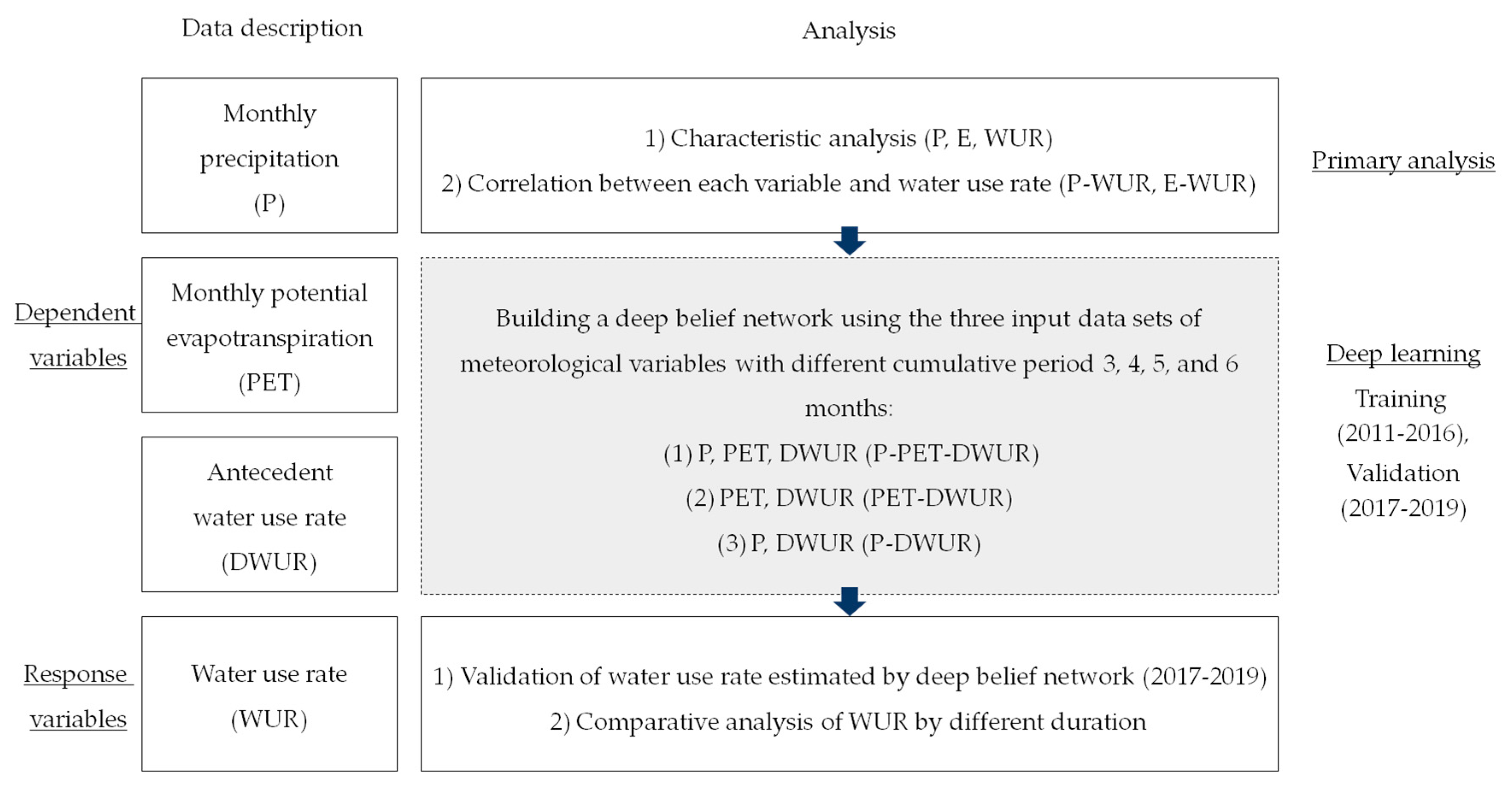
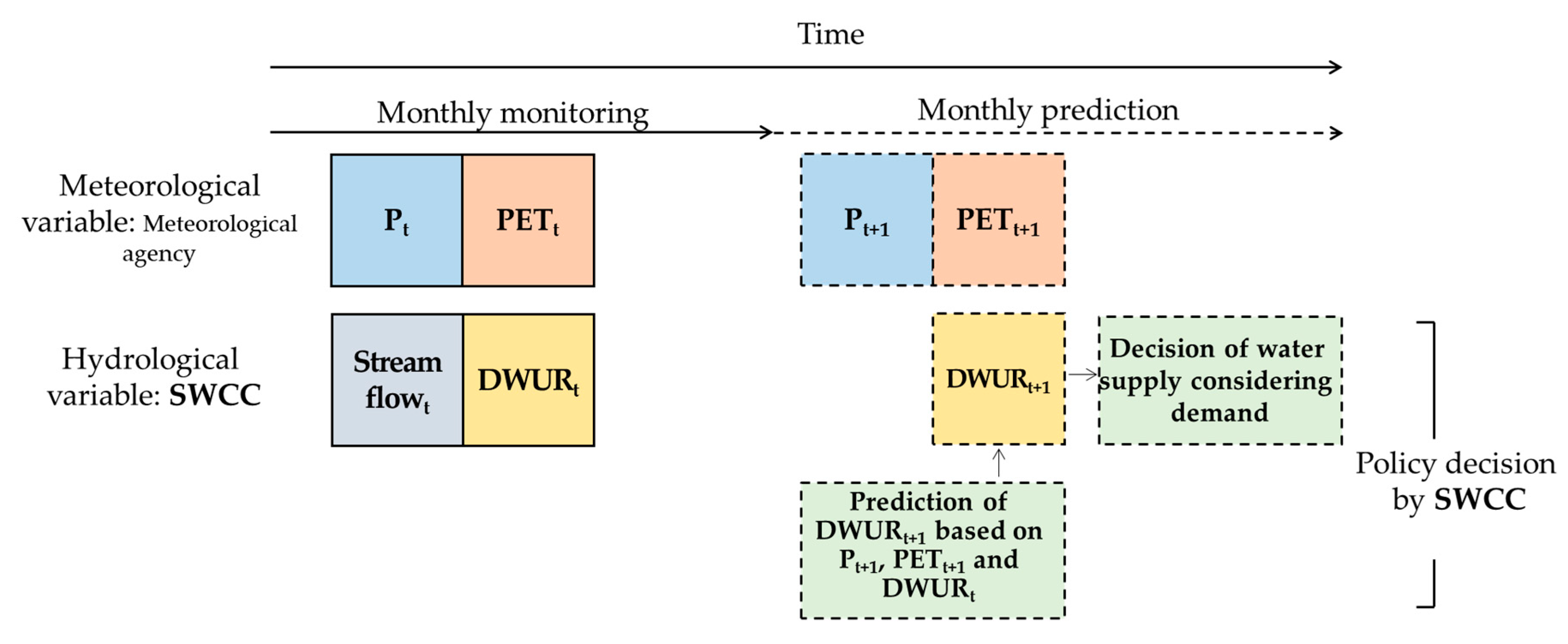
2.1. Experimental Design

This study proposed a deep learning-based prediction model of WUR by considering weather variables and evaluated its reproducibility. We found relationships among WUR and meteorological variables such as precipitation (P) and potential evapotranspiration (PET) for nine years (2011–2019). Moreover, a new model using DBN, an unsupervised method to train with a relatively small dataset, was developed for predicting WUR. The training and prediction periods for the DBN were 2011 to 2016, and 2017 to 2019, respectively. The prediction variable was WUR, and the input variables were combinations of precipitation (P) and PET for various time durations (3-, 4-, 5-, and 6-month cumulative) including DWUR that accounts for a month before the prediction month [32]. Because drought occurs due to an excessive shortage of accumulative precipitation and continuously active evapotranspiration, monthly cumulative P and PET for 3, 4, 5, and 6 months were used as input datasets. Therefore, this study used the following three possible input datasets: (1) P, PET, and DWUR (P-PET-DWUR), (2) PET and DWUR (PET-DWUR), and (3) P and DWUR (P-DWUR). The objectives of this study were to identify the relationships among WUR and meteorological variables and to suggest the DBN-based prediction model with the best input dataset using different cumulative periods in the Yeongsan River basin. Moreover, this prediction model was applied to several water-use facilities for its validation (Figure 1).

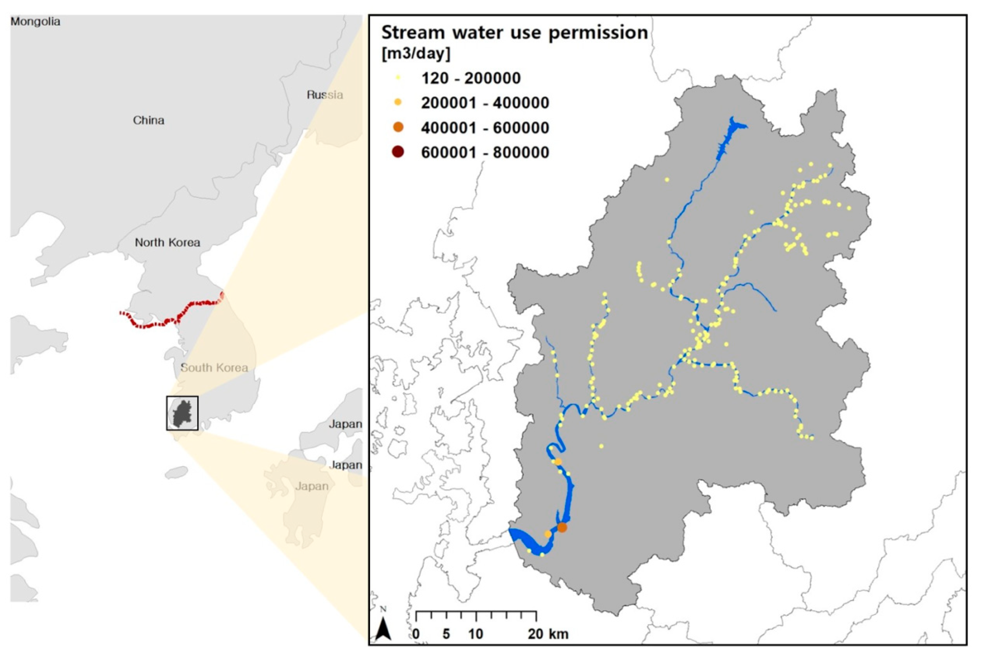
2.2. Study Area and Data

To secure a reliable supply of stream water (i.e., agricultural water), the central government permits and manages stream water in Korea. The upper limit boundary of available stream water use is set as the reference low flow to prevent indiscriminate water use and reduce stream water deficit. The reference low flow is defined by the ten-year frequency streamflow that is maintained for more than 355 days per year [33]. Although use of stream water is permitted below the reference low flow, the water-use facility (WUF) controls the amount of stream water used according to drought severity.

The flood control office has responsibility for managing stream water and adjusting the permitted amount for the WUFs. The amount of permitted stream water for each WUF can be changed every year with consideration of both water demand and water availability by the authority of the institutions. Unlike stream water use, the WUR is defined as stream water use (demand) divided by stream water permit (supply), in the range 0 to 100. Therefore, the WUR was chosen to be the prediction variable instead of stream water use. The Yeongsan River basin located in southwestern Korea is well known as a large-scale agricultural region even after industrialization. Stream water has been highly demanded near the downstream of the river basin where the population is concentrated along the riverside (Figure 2).

In this study, the meteorological variables were precipitation and potential evapotranspiration (PET), observed from twelve automated surface observing systems in the Korea Meteorological Administration. The basin mean monthly precipitation was calculated by using the Thiessen method. Monthly PET was estimated by the Thornthwaite equation [34] using observed monthly mean temperature at the stations in the basin. The stream water use by WUFs was averaged and used for the model input data as antecedent WUR.

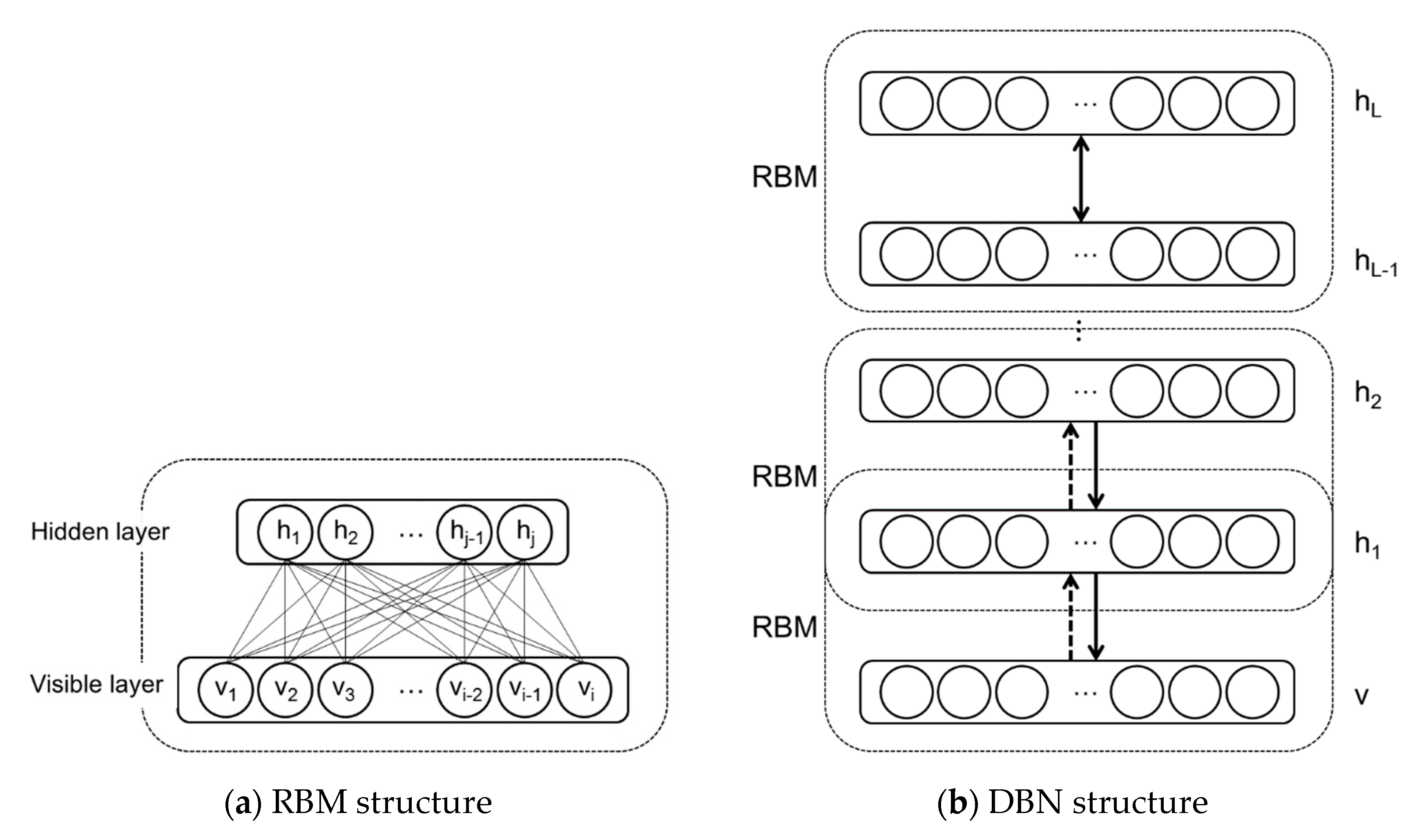
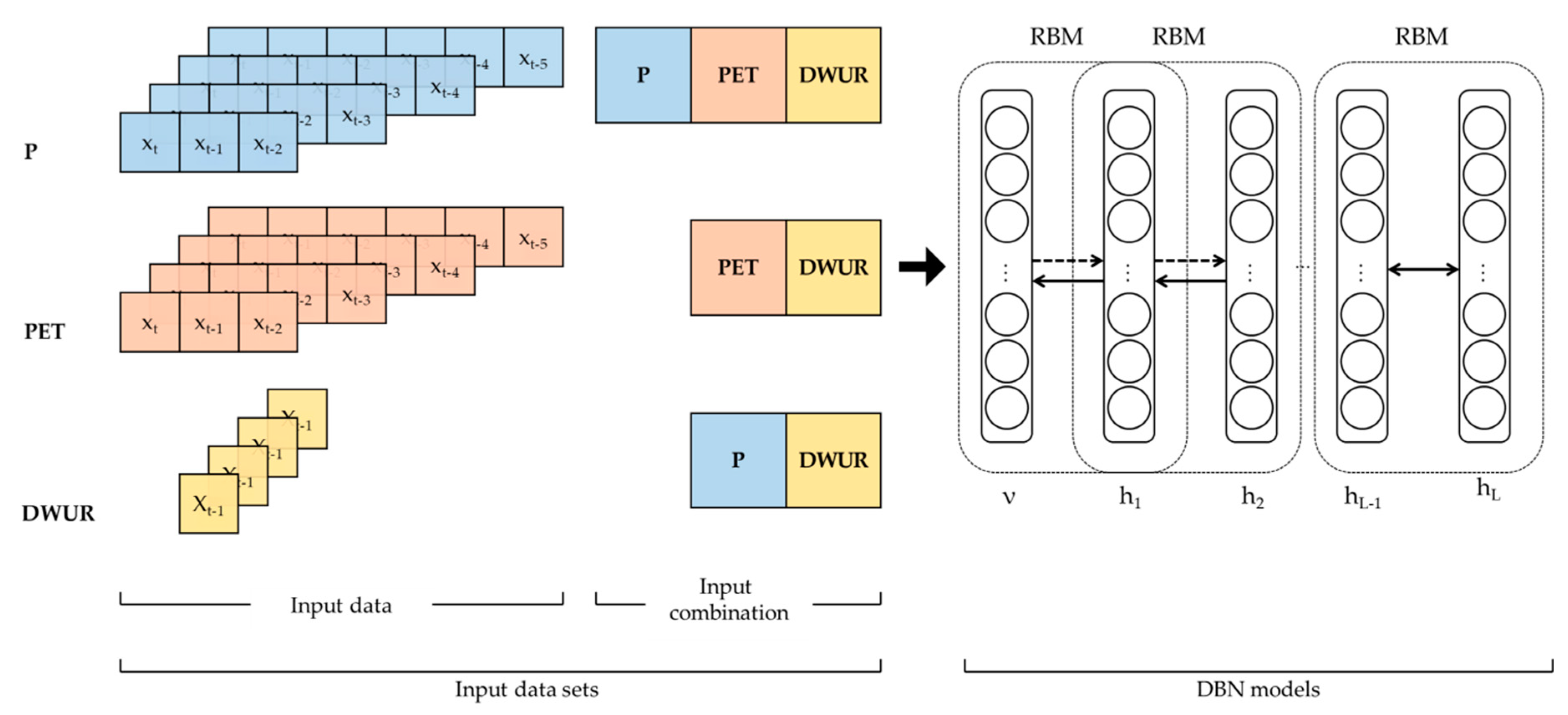
2.3. Deep Belief Network (DBN)

A DBN is a probabilistic generative model that has several stacked RBMs and it trains using the greedy learning method. A RBM is a type of Markov model that has no edges in each layer, unlike Boltzmann machine which has a connection between layers [35]. A RBM expresses a joint probability distribution using a graph consisting of nodes corresponding to random variables and edges representing the relationships among random variables and it consists of one visible layer and one hidden layer. Here, visible units are input data, and hidden units are outputs that improve learning ability (Figure 3a). DBN is a structure that stacks RBM with a simple calculation process, unlike deep Boltzmann machine (DBM) which expresses the entire layer as joint probability, and the rest of the layers, except the last layer, are expressed as conditional probability as follows:

$$P\left(\nu , h^1, \cdots , h^L\right)=\left({{\displaystyle \prod }}_{l=1}^{L-2}P(h^{l-1}|h^l)P\left(h^{L-1},h^L\right)\right),$$

(1)

where $h^0= \nu$, $L$ is number of hidden layers, $P(h^{l-1}|h^l)$ denotes the conditional distribution for the units of the layer $\left(l-1\right)$ given the $l$ units layer, and $P\left(h^L,h^{L-1}\right)$ corresponds to the joint distribution of the top two layers $\left(L-1\right) \mathrm{and} L$.

The input data initializes the weights of the DBN by the pretraining step before the backpropagation algorithm is used to fine-tune the weights in the learning phase. Hence, the initial weight is determined, and the next layer is trained. This process is repeated until all the layers are trained (Figure 3b).

DBN training is a layer-wise pretraining technique that sequentially performs pretraining from the lower layer (the layer close to the input) to the upper layer. The initial weight is pretrained using a layer-by-layer strategy, and the higher-level features are trained from the previous layers.

The DBN training process can be summarized as follows:

1. To initialize the visible units to a training dataset;

2. To express the back-and-forth process as a conditional probability

$$\mathrm{Positive} \mathrm{phase}, P\left(\nu \right)= \sigma \left(c_j+{\displaystyle \sum }{\omega }_{ij}{\nu }_i\right),$$

(2)

$$\mathrm{Negative} \mathrm{phase}, P\left(h\right)= \sigma \left(b_j+{\displaystyle \sum }{\omega }_{ij}{\nu }_i\right)$$

(3)

where $\sigma$ is the activation transfer function, $c_j$ and $b_i$ are the biases, ${\nu }_i$ and $h_j$ are the states of the visible and hidden units, and ${\omega }_{ij}$ represents the connection weight between units i and j;

3. To re-update all of the hidden units in parallel given the reconstructed visible units using Equation (2); and

4. To repeat with all training examples and update the weights (${\omega }_{ij}$) and biases ($c_j$ and $b_i$) using Equations (4)–(6),

$$\mathsf{\Delta }{\omega }_{ij}=\alpha \left({\langle {\nu }_i{h}_j\rangle }_{data}-{\langle {\nu }_i{h}_j\rangle }_{recon}\right),$$

(4)

$$\mathsf{\Delta }{c}_j=\alpha \left({\langle h_j\rangle }_{data}-{\langle h_j\rangle }_{recon}\right),$$

(5)

$$\mathsf{\Delta }{b}_i=\alpha \left({\langle {\nu }_i\rangle }_{data}-{\langle {\nu }_i\rangle }_{recon}\right),$$

(6)

where $\langle ·\rangle$ denotes the expectation of the training data, ${\langle {\nu }_i{h}_j\rangle }_{data}$ refers to the distribution of raw data input to the RBM, ${\langle {\nu }_i{h}_j\rangle }_{recon}$ refers to the distribution of data after the model has been reconstructed, and $\alpha$ is learning rate.

This study applied the DEEPNET library of the R program to estimate the WUR. The proposed DBN settings are shown in

Table 1. Description of deep learning parameter settings.

Items	Detail
Prediction variable	Stream water-use rate (WUR)
Input variable	3-, 4-, 5-, and 6-month cumulative precipitations (P) 3-, 4-, 5-, and 6-month cumulative PETs (PET) Antecedent stream water-use rate (DWUR)
Training parameters	Number of hidden units: 10, 20, 30 Learning rate: 0.1, 0.5, 0.9 Number of epochs: 100, 500, 1000 Batch size: 6, 12, 24

. The prediction variable was the WUR, and the input variables were combinations of precipitation (P) and PET for various time durations (3-, 4-, 5-, and 6-month cumulative) including DWUR that accounts for a month before the prediction month. Each model updated over a different range of hidden units, learning rates, epochs, batch sizes on the same underlying input set to select the optimal parameters. The training period was 2011–2016, and the DBN model was validated from 2017 to 2019. Therefore, twelve models based on combinations of input variables were constructed to estimate the WUR (Figure 4).

3. Results

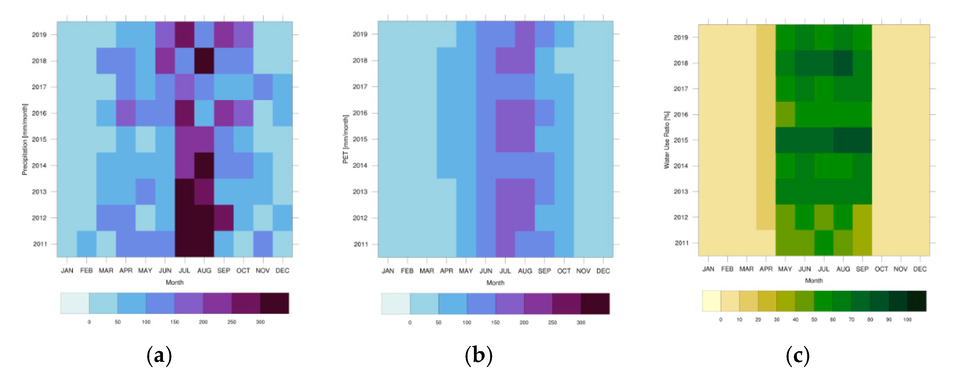
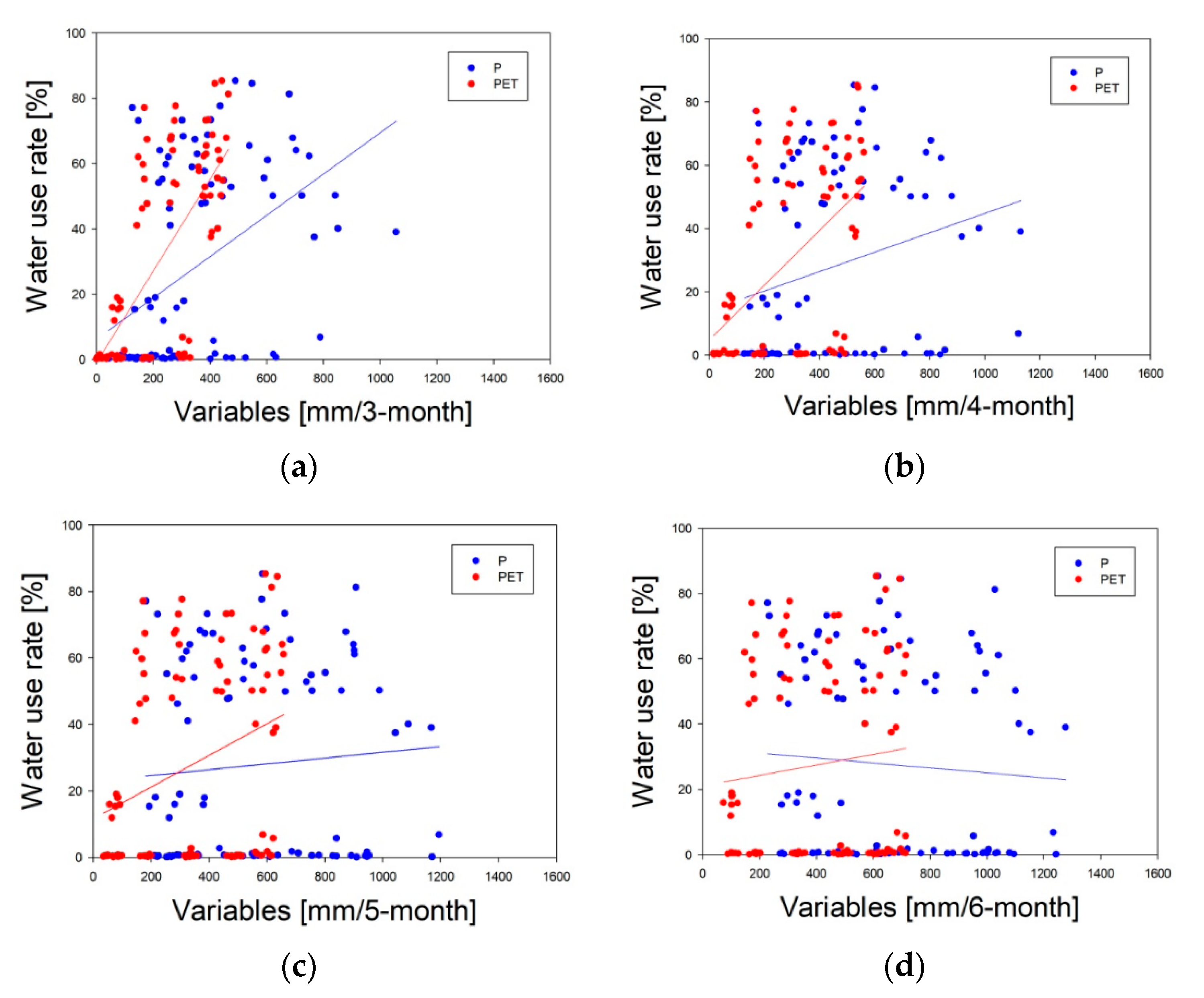
3.1. Relationship between Meteorological Variables and Stream Water-Use Rate

This study used the monthly precipitation, monthly PET, and monthly WUR from 2011 to 2019 (Figure 5). The monthly mean precipitation ranged from 22.9 to 262.4 mm, mainly concentrated in July and August which was 40% (516.79 mm) of the annual precipitation (1301.9 mm) (Figure 5a). The monthly PET started to increase from April and largely occurred in July and August which was 55% (310.4 mm) of the total annual PET (787.8 mm) (Figure 5b). The WUR underwent the annual cycle of agricultural activities, which increased from May to September (Figure 5c). The annual mean WUR was 26.7% with peaks of 63.2% in June. Especially, the highest WUR was in 2015, when extreme drought was experienced in South Korea [4].

Correlation coefficients were obtained to examine the relationships among P/PET and WUR for different durations. The relationship became weaker as the accumulated period was longer (Figure 6). The correlations of WUR with P and PET, for a 3-month duration, were 0.47 and 0.72, respectively; those for the four-, five-, and six-month cumulative durations were 0.28 and 0.54, 0.09 and 0.33, and −0.07 and 0.12, respectively. In particular, the WUR was strongly correlated with accumulated PET over three months, because increased PET caused the soil to be drier, which resulted in the manager of the WUF perceiving an increased demand for the crops. As the cumulative period was extended, the slope of the regression line for precipitation was significantly changed as compared with that of PET. In particular, the six-month cumulative period showed a negative relationship.

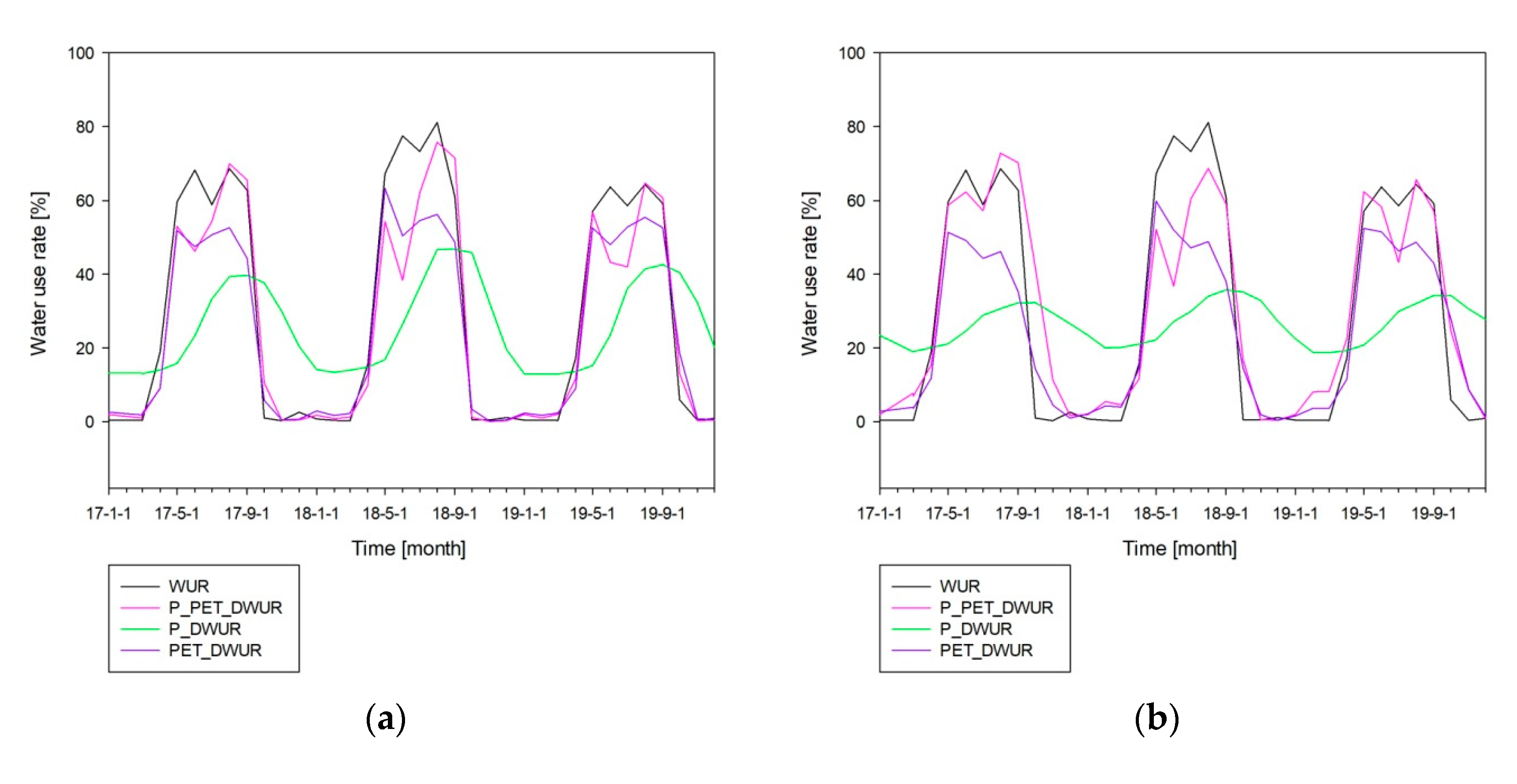
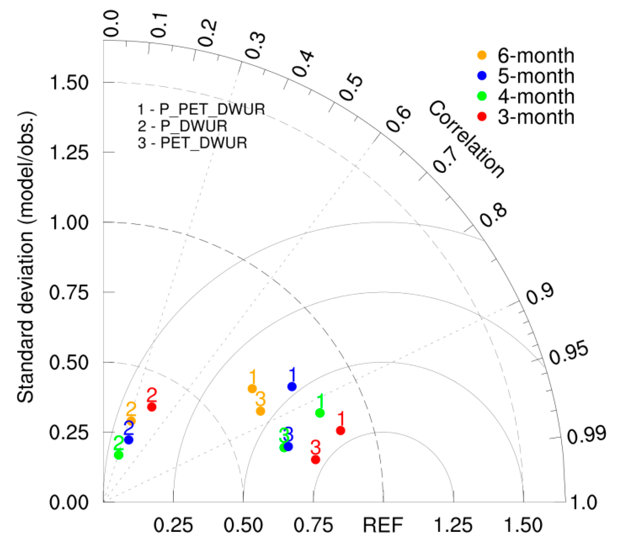
3.2. Estimation of Stream Water-Use Rate

We constructed a DBN-based model using precipitation and PET to estimate WUR. We selected the optimal parameters for the DBN based on the best performance model, as shown in

Table 2. Optimal parameters of the deep belief network (DBN).

Parameters	Duration	P_PET_DWUR	P_DWUR	PET_DWUR
Hidden layer	3 months	20	10	20
	4 months	20	10	30
	5 months	30	30	10
	6 months	10	20	20
Learning rate	3 months	0.9	0.5	0.5
	4 months	0.9	0.9	0.5
	5 months	0.9	0.5	0.9
	6 months	0.5	0.5	0.9
Epochs	3 months	1000	100	1000
	4 months	1000	100	1000
	5 months	1000	1000	1000
	6 months	1000	1000	1000
Batch size	3 months	6	6	6
	4 months	12	24	6
	5 months	12	6	6
	6 months	12	6	6

. The optimal parameters differed by accumulated meteorological variables for various time durations (3, 4, 5, and 6 months).

Figure 7 shows a time series of WUR by different cumulative periods for 3, 4, 5, and 6 months, to compare the estimated three different combinations of meteorological variables for each duration. The precipitation, PET, and DWUR of a three-months cumulative period estimated the most similar to the observations. In addition, the estimated WUR by PET-DWUR for the three-month cumulative period was similar to the observations (Figure 7a). P-DWUR inferred that the estimated WUR was underestimated as compared with the observations, and it showed some lagged response. The longer the cumulative duration of the meteorological variables, the lower the performance skill of the model. Especially, the P-DWUR showed a lower predictability with a relatively shorter cumulative period than the others.

For quantitative performance evaluation of the DBN model based on input data for each duration, it was diagnosed using root mean square error (RMSE), Nash–Sutcliff efficiency (NSE), and determination coefficient (R²) (

Table 3. Results of the prediction model in the validation period.

Duration	Performance Index	P_PET_DWUR	P_DWUR	PET_DWUR
3 months	RMSE	0.12	0.33	0.12
	NSE	0.90	0.18	0.89
	R2	0.92	0.21	0.96
4 months	RMSE	0.14	0.35	0.16
	NSE	0.85	0.07	0.81
	R2	0.85	0.10	0.92
5 months	RMSE	0.19	0.34	0.16
	NSE	0.72	0.12	0.81
	R2	0.73	0.14	0.92
6 months	RMSE	0.23	0.35	0.21
	NSE	0.61	0.10	0.68
	R2	0.63	0.11	0.75

). The RMSEs or NSEs of the estimated WUR with P-PET-DWUR and PET-DWUR, at the three-month cumulative period, were similar, and the R² of WUR between observation and estimation with PET-DWUR was 0.96, which showed a strong positive relationship. This result reflects the phenomenon that WUR increases as PET increases. It can be seen that the model performance decreases as the duration increases. In particular, the correlations among cumulative precipitation and PET, and WUR decreased as the duration increased, as shown in Figure 6b–d. Additionally, as the RMSE increased and the NSE decreased, the performances of the model for different durations were reduced. The scores of inferred WUR by PET-DWUR also decreased according to the increased cumulative duration, but it showed better performance than those of P-DWUR with all performance indices.

The Taylor diagram represents the model performance for the estimated WUR which can reflect the correlation, the ratio of the standardized deviation, and centered RMS difference (CRMSD) [36]. The correlation coefficient between the modeled and the observed data is visualized by cos θ which is the azimuth angle (θ) of each point, and a circle is drawn around the reference point (REF) representing CRMSD. The CRMSD is the RMSD that does not take into account the mean model bias, and CRMSD is divided with observed standard deviation, as shown in Figure 8 Therefore, the most ideal value is at REF, where the correlation coefficient is 1, the ratio of standard deviation is 1, and the CRMSD is 0.

The PET-DWUR model had a higher correlation coefficient than the P-PET-DWUR model for all cumulative periods, while the P-PET-DWUR model had a higher ratio of the standard deviation than the PET-DWUR model for all cumulative periods. The CRMSDs of both the PET-DWUR and P-PET-DWUR models for the three- and four-month cumulative durations were similar, however, the CRMSDs of PET-DWUR for the five- and six-month cumulative durations were lower than those of P-PET-DWUR (Figure 8). The PET-DWUR showed better performance than P-PET-DWUR for five- and six-month cumulative durations. Both P-PET-DWUR and PET-DWUR for the three-month cumulative duration showed the best performance, the correlations were 0.96 and 0.98; the ratios of standard deviation were 0.88, and 0.77; and the CRMSDs were 0.30 and 0.29, respectively. The performance of estimated WUR based on both P-PET-DWUR and PET-DWUR showed close to the REF. The P-PET-DWUR and the PET-DWUR for the four-month cumulative duration showed a similar distance to the REF.

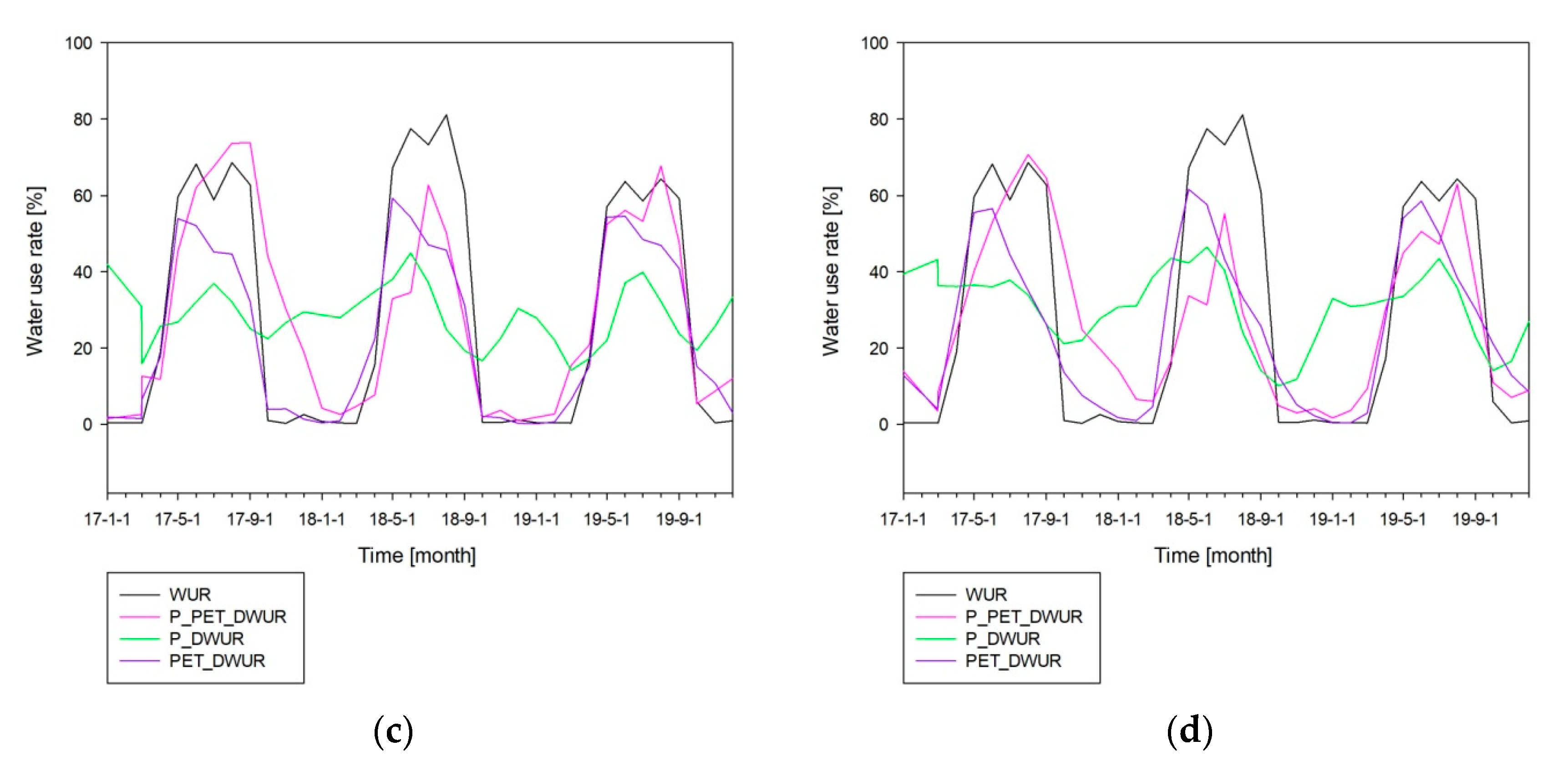
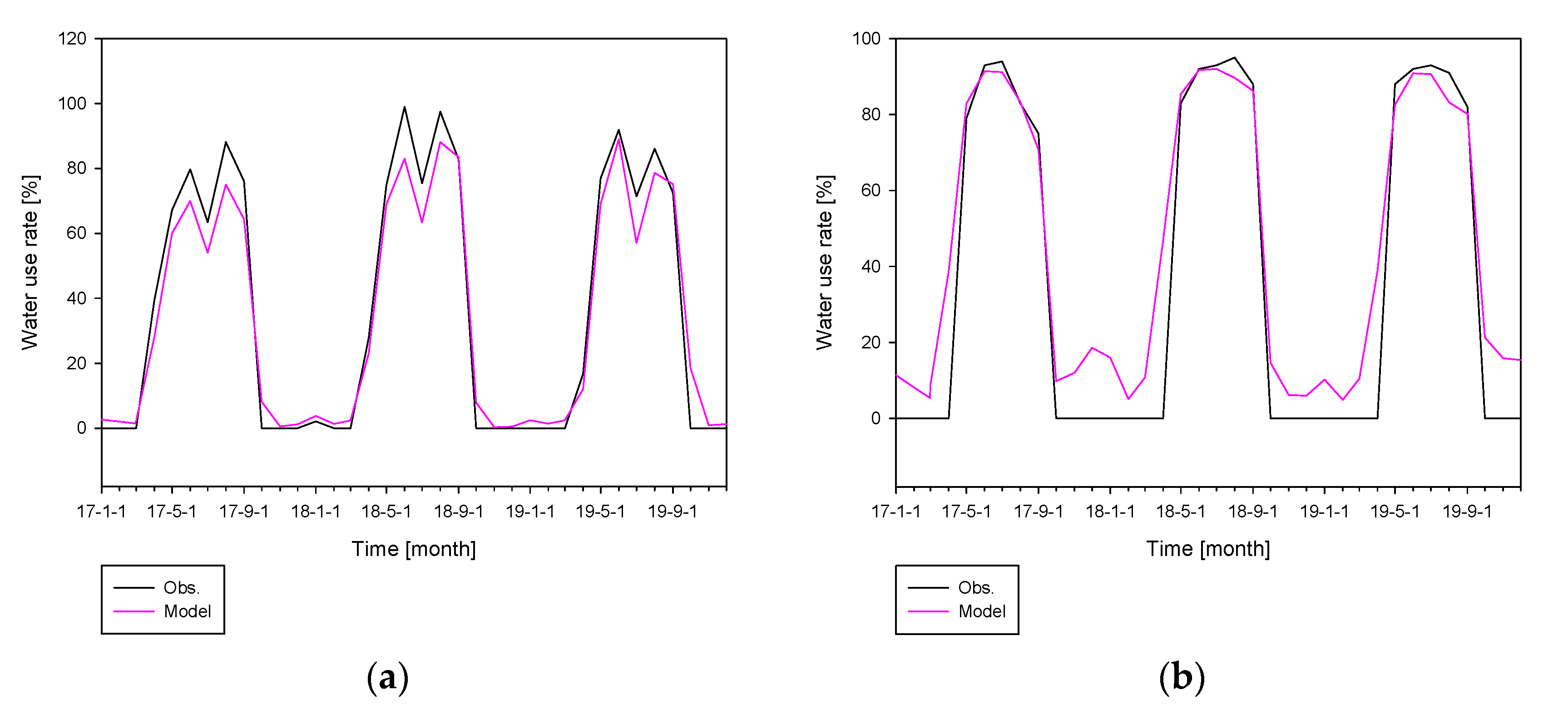
3.3. Estimation of Stream Water-Use Rate on Stream Water-Use Facilities

The model using P-PET-DWUR and PET-DWUR for the three-month cumulative period as input data showed excellent performances for WUR. The inferred WUR is the average of all the WUFs in the Yeongsan River basin. In order to examine the applicability of the DBN model, WUR was estimated by two single facilities. We selected the facilities that had a small annual variance of WUR in the Yeongsan River basin. The stream water-use permits of the selected WUFs, Si-Jong (st. 926) and Wol-Ho (st. 976), were 979,935 and 494,144 m³/day, and WURs were 35.8% and 36.7%, respectively. To examine the effectiveness of the DBN model at each WUF, the DBN model using PET-DWUR for the three-month cumulative period had the best performance as compared with the other durations estimated WUR with the observations from 2017 to 2019 (Figure 9a,b).

The RMSEs of estimated WUR were 0.76 (st. 926) and 0.15 (st. 976), NSEs were 0.96 (st. 926) and 0.88 (st. 976), and R² were 0.97 (st. 926) and 0.94 (st. 976), respectively. The performances of the model showed its excellence to predict WUR at each WUF. However, the irrigation pumping facility, st. 927, withdrew stream water only from May to September and there was no stream water use for the remaining months, which caused the model to overestimate the WUR from October to April. In addition, the accuracy of the inferred WUR from May to September was very high as the WUR tended to constantly be high.

4. Conclusions

This study proposed a DBN-based model to estimate WUR in the Yeongsan River basin with a high proportion of agricultural land use. Specifically, on the basis of relationships among meteorological variables and WUR, a deep learning-based model was developed to estimate WUR using precipitation and PET. For the relationship between WUR and precipitation, PET having three-month cumulative durations was the strongest. Overall, the relationship became weaker as the accumulated period became longer. Within the same cumulative period, the correlation of WUR with PET was higher than with precipitation because most of the basin consisted of well-irrigated paddy fields where the water could be safely supplied even during droughts. The well-irrigated paddy was less sensitive to the lack of precipitation because water could be stably supplied for agricultural use even if the precipitation was relatively small. Therefore, stream water users demand more water when PET increases, leading to dryness of soil moisture.

In this study, stream water use was estimated by applying DBN for the derivation of the relationships among the quantified meteorological variables and WUR. The best performance was for three-month accumulated precipitation and PET. The results using P-PET-DWUR and PET-DWUR showed the best performance, and the P-DWUR based estimate of WUR revealed a relatively poorer performance than PET-DWUR. When the cumulative period was over four months, the estimated WUR with PET-DWUR showed better performance as compared with that of both precipitation and PET. This matches previous results that showed the relationship between WUR and two meteorological variables, precipitation and PET. The SWCC, the governance-based agency in South Korea, can operationally adjust stream water use with a soft-path approach. However, the operation of the SWCC has been ineffective due to difficulty predicting stream water use. The estimation method for WUR was developed based on relationships with meteorological variables, and its applicability was verified. The proposed method showed the possibility for forecasting WUR considering weather conditions, and accordingly, it could be actively used to adjust the amount of stream water use as a soft-path solution (Figure 10).

A limitation of this study was that only agricultural water use was considered, and other water uses were excluded, i.e., residential, environmental, and industrial water use. We confirmed that the proposed model using PET-DWUR could be effectively applied to predict agricultural water-use. However, it is necessary to consider all types of crops that could cause different patterns of stream water use.

References

1. Milly, P.C.D.; Betancourt, J.; Falkenmark, M.; Hirsch, R.M.; Kundzewicz, Z.W.; Lettenmaier, D.P.; Stouffer, R.J. Stationarity is dead: Whither water management? Science 2008, 319, 573–574. [Google Scholar] [CrossRef] [PubMed]
2. Sung, J.H.; Chung, E.S.; Lee, B.; Kim, Y. Meteorological hazard risk assessment based on the detection of trends and abrupt changes in the precipitation characteristics of the Korea peninsula. Theoret. Appl. Climatol. 2017, 127, 305–326. [Google Scholar] [CrossRef]
3. Abdulai, P.J.; Chung, E.S. Uncertainty assessment in drought severities for the Cheongmicheon watershed using multiple GCMs and the reliability ensemble averaging method. Sustainability 2019, 11, 4283. [Google Scholar] [CrossRef] [Green Version]
4. Kwon, H.-H.; Lall, U.; Kim, S.-J. The unusual 2013–2015 drought in South Korea in the context of a multicentury precipitation record: Inferences from a nonstationary, multivariate, Bayesian copula model. Geophys. Res. Lett. 2016, 43, 8534–8544. [Google Scholar] [CrossRef]
5. Sung, J.H.; Chung, E.S. Development of streamflow drought severity-duration-frequency curves using the threshold level method. Hydrol. Earth Syst. Sci. 2014, 18, 3341–3351. [Google Scholar] [CrossRef] [Green Version]
6. Sung, J.H.; Chung, E.S.; Shahid, S. Reliability–resiliency–vulnerability approach for drought analysis in South Korea using 28 GCMs. Sustainability 2018, 10, 3043. [Google Scholar] [CrossRef] [Green Version]
7. Gleick, P.H.; Burns, W.C.G.; Chalecki, E.L.; Cohen, M.; Cushing, K.K.; Mann, A.S.; Reyes, R.; Wolff, G.H.; Wong, A.K. The World’s Water 2002–2003: The Biennial Report on Freshwater Resources; Island Press: Washington, DC, USA, 2002; ISBN 978-1-55963-949-1. [Google Scholar]
8. Cooley, H.; Fulton, J.; Gleick, P.H. Water for Energy: Future Water Needs for Electricity in the Intermountain West; The Pacific Institute: Oakland, CA, USA, 2011; pp. 1–63. [Google Scholar]
9. Wutich, A.; White, A.C.; White, D.D.; Larson, K.L.; Brewis, A.; Roberts, C. Hard paths, soft paths or no paths? Cross-cultural perceptions of water solutions. Hydrol. Earth Syst. Sci. 2014, 18, 109–120. [Google Scholar] [CrossRef] [Green Version]
10. Brooks, D.B.; Holtz, S. Water soft path analysis: From principles to practice. Water Int. 2009, 34, 158–169. [Google Scholar] [CrossRef]
11. Hong, C.-Y.; Chang, H.; Chung, E.-S. Resident perceptions of urban stream restoration and water quality in South Korea. River Res. Appl. 2018, 34, 481–492. [Google Scholar] [CrossRef]
12. Keyantash, J.; Dracup, J.A. The quantification of drought: An evaluation of drought indices. Bull. Am. Meteorol. Soc. 2002, 83, 1167–1180. [Google Scholar] [CrossRef]
13. Vasiliades, L.; Loukas, A. Hydrological response to meteorological drought using the Palmer drought indices in Thessaly, Greece. Desalination 2009, 237, 3–21. [Google Scholar] [CrossRef]
14. Vicente-Serrano, S.M.; Beguería, S.; Lorenzo-Lacruz, J.; Camarero, J.J.; López-Moreno, J.I.; Azorin-Molina, C.; Revuelto, J.; Morán-Tejeda, E.; Sanchez-Lorenzo, A. Performance of drought indices for ecological, agricultural, and hydrological applications. Earth Interact. 2012, 16, 1–27. [Google Scholar] [CrossRef] [Green Version]
15. LeCun, Y.; Bengio, Y.; Hinton, G. Deep learning. Nature 2015, 521, 436–444. [Google Scholar] [CrossRef] [PubMed]
16. Bengio, Y.; Lamblin, P.; Popovici, D.; Larochelle, H. Greedy layer-wise training of deep networks. In Proceedings of the 19th International Conference on Neural Information Processing Systems, Vancouver, BC, Canada, 4–7 December 2006; MIT Press: Cambridge, MA, USA, 2006; pp. 153–160. [Google Scholar]
17. Ranzato, M.; Poultney, C.; Chopra, S.; LeCun, Y. Efficient Learning of Sparse Representations with an Energy-Based Model. In Proceedings of the 19th International Conference on Neural Information Processing Systems, Vancouver, BC, Canada, 4–7 December 2006; MIT Press: Cambridge, MA, USA, 2006; pp. 1137–1144. [Google Scholar]
18. Partal, T.; Cigizoglu, H.K. Estimation and forecasting of daily suspended sediment data using wavelet–neural networks. J. Hydrol. 2008, 358, 317–331. [Google Scholar] [CrossRef]
19. Barua, S.; Perera, B.J.C.; Ng, A.W.M.; Tran, D. Drought forecasting using an aggregated drought index and artificial neural network. J. Water Clim. Chang. 2010, 1, 193–206. [Google Scholar] [CrossRef]
20. Tiwari, M.K.; Chatterjee, C. Development of an accurate and reliable hourly flood forecasting model using wavelet–bootstrap–ANN (WBANN) hybrid approach. J. Hydrol. 2010, 394, 458–470. [Google Scholar] [CrossRef]
21. Adamowski, J.; Chan, H.F. A wavelet neural network conjunction model for groundwater level forecasting. J. Hydrol. 2011, 407, 28–40. [Google Scholar] [CrossRef]
22. Rajaee, T.; Nourani, V.; Zounemat-Kermani, M.; Kisi, O. River suspended sediment load prediction: Application of ann and wavelet conjunction model. J. Hydrol. Eng. 2011, 16, 613–627. [Google Scholar] [CrossRef]
23. Jothiprakash, V.; Magar, R.B. Multi-time-step ahead daily and hourly intermittent reservoir inflow prediction by artificial intelligent techniques using lumped and distributed data. J. Hydrol. 2012, 450–451, 293–307. [Google Scholar] [CrossRef]
24. Kim, S.; Seo, Y.; Singh, V.P. Assessment of pan evaporation modeling using bootstrap resampling and soft computing methods. J. Comput. Civ. Eng. 2015, 29, 04014063. [Google Scholar] [CrossRef]
25. Seo, Y.; Kim, S.; Kisi, O.; Singh, V.P.; Parasuraman, K. River stage forecasting using wavelet packet decomposition and machine learning models. Water Resour. Manag. 2016, 30, 4011–4035. [Google Scholar] [CrossRef]
26. Le, X.-H.; Ho, H.V.; Lee, G.; Jung, S. Application of Long Short-Term Memory (LSTM) neural network for flood forecasting. Water 2019, 11, 1387. [Google Scholar] [CrossRef] [Green Version]
27. Song, Y.H.; Chung, E.-S.; Shiru, M.S. Uncertainty Analysis of Monthly Precipitation in GCMs Using Multiple Bias Correction Methods under Different RCPs. Sustainability 2020, 12, 7508. [Google Scholar] [CrossRef]
28. Hinton, G.E.; Osindero, S.; Teh, Y.-W. A fast learning algorithm for deep belief nets. Neural Comput. 2006, 18, 1527–1554. [Google Scholar] [CrossRef] [PubMed]
29. Chen, J.; Jin, Q.; Chao, J. Design of deep belief networks for short-term prediction of drought index using data in the huaihe river basin. Math. Probl. Eng. 2012, 2012, 235929. [Google Scholar] [CrossRef] [Green Version]
30. Agana, N.A.; Homaifar, A. EMD-based predictive deep belief network for time series prediction: An application to drought forecasting. Hydrology 2018, 5, 18. [Google Scholar] [CrossRef] [Green Version]
31. Xu, Y.; Zhang, J.; Long, Z.; Chen, Y. A novel dual-scale deep belief network method for daily urban water demand forecasting. Energies 2018, 11, 1068. [Google Scholar] [CrossRef] [Green Version]
32. Gers, F.A.; Eck, D.; Schmidhuber, J. Applying LSTM to time series predictable through time-window approaches. In Proceedings of the Neural Nets WIRN Vietri-01, Vienna, Austria, 21–25 August 2001; Tagliaferri, R., Marinaro, M., Eds.; Springer: London, UK, 2002; pp. 193–200. [Google Scholar]
33. Sung, J.H.; Seo, S.B. Estimation of river management flow considering stream water deficit characteristics. Water 2018, 10, 1521. [Google Scholar] [CrossRef] [Green Version]
34. Thornthwaite, C.W. An approach toward a rational classification of climate. Geogr. Rev. 1948, 38, 55–94. [Google Scholar] [CrossRef]
35. Smolensky, P. Information processing in dynamical systems: Foundations of harmony theory. In Parallel Distributed Processing: Explorations in the Microstructure of Cognition, Volume 1: Foundations; MIT Press: Cambridge, MA, USA, 1986; pp. 194–281. ISBN 978-0-262-68053-0. [Google Scholar]
36. Taylor, K.E. Summarizing multiple aspects of model performance in a single diagram. J. Geophys. Res. Atmos. 2001, 106, 7183–7192. [Google Scholar] [CrossRef]
Figure 1. Procedure of this study.
Water 12 02700 g001
Figure 2. Location of Yeongsan River basin with the stream water-use facilities.
Water 12 02700 g002
Figure 3. Structure of (a) restricted Boltzmann machine (RBM) and (b) deep belief network with stacked multiple RBMs.
Water 12 02700 g003
Figure 4. Proposed deep belief network configuration.
Water 12 02700 g004
Figure 5. Matrix plot for monthly (a) precipitation, (b) potential evapotranspiration, and (c) stream water-use rate, from 2011 to 2019.
Water 12 02700 g005
Figure 6. Scatter plots describing the relationships among precipitation and potential evapotranspiration and stream water-use rate for different cumulative durations. (a) 3-month cumulative; (b) 4-month cumulative; (c) 5-month cumulative; (d) 6-month cumulative.
Water 12 02700 g006
Figure 7. Comparison between the observed and estimated stream water-use rate in the validation period. (a) 3-month cumulative; (b) 4-month cumulative; (c) 5-month cumulative; (d) 6-month cumulative.
Water 12 02700 g007aWater 12 02700 g007b
Figure 8. Performance of simulated water-use rate WUR statistics in the validation period over Yeongsan River basin.
Water 12 02700 g008
Figure 9. Comparison between the observed and estimated WUR. (a) At st. 926; (b) At st. 976.
Water 12 02700 g009
Figure 10. Monitoring and decision making by the stream water coordination council (SWCC).
Water 12 02700 g010