Article

Dynamical Modeling of Water Flux in Forward Osmosis with Multistage Operation and Sensitivity Analysis of Model Parameters

1
Department of Chemical and Biomolecular Engineering, KAIST, 291 Daehak-ro, Yuseong-gu, Daejeon 34141, Korea
2
Department of Civil and Environmental Engineering, KAIST, 291 Daehak-ro, Yuseong-gu, Daejeon 34141, Korea
3
Samsung Electronics, 1-1, Samsungjeonja-ro, Hwaseong-si 18448, Gyeonggi, Korea
4
Advanced Biomass R&D Center, #2502 Building W1-3, 291 Daehak-ro, Yuseong-gu, Daejeon 34141, Korea
*
Authors to whom correspondence should be addressed.
Water 2020, 12(1), 31; https://doi.org/10.3390/w12010031
Submission received: 11 November 2019 / Revised: 16 December 2019 / Accepted: 16 December 2019 / Published: 19 December 2019
(This article belongs to the Section Water Use and Scarcity)

Abstract

:
To mathematically predict the behavior of a forward osmosis (FO) process for water recovery, a model was constructed using an asymmetric membrane and glucose as a draw solution, allowing an examination of both phenomenological and process aspects. It was found that the proposed model adequately described the significant physicochemical phenomena that occur in the FO system, including forward water flux, internal concentration polarization (ICP), external concentration polarization (ECP), and reverse solute diffusion (RSD). Model parameters, namely the physiochemical properties of the FO membrane and glucose solutions, were estimated on the basis of experimental and existing data. Through batch FO operations with the estimated parameters, the model was verified. In addition, the influences of ECP and ICP on the water flux of the FO system were investigated at different solute concentrations. Water flux simulation results, which exhibited good agreement with the experimental data, confirmed that ICP, ECP, and RSD had a real impact on water flux and thus must be taken into account in the FO process. With the Latin-hypercube—one-factor-at-a-time (LH–OAT) method, the sensitivity index of diffusivity was at its highest, with a value of more than 40%, which means that diffusivity is the most influential parameter for water flux of the FO system, in particular when dealing with a high-salinity solution. Based on the developed model and sensitivity analysis, the simulation results provide insight into how mass transport affects the performance of an FO system.

Graphical Abstract

1. Introduction

Water shortages have become a key issue facing humanity. According to the United Nations World Water Development Report in 2019, over 2 billion people suffer from severe water shortage, and the global demand for fresh water has been increasing by about 1% annually since the 1980s [1]. Consequently, much effort has been made to secure water, in particular safe water, with low energy consumption. One such means is membrane-based water treatment and desalination technology, which is relatively energy-efficient and independent of the water cycle [2].
Several types of membrane-based desalination technology, including electrodialysis, membrane distillation, reverse osmosis (RO), and forward osmosis (FO), have been developed [3,4]. Among these, FO-based water desalination, of which the driving force is an intrinsic osmotic pressure gradient, has a unique position because (1) it is highly resistant to membrane fouling [5], (2) it requires much lower energy [6] and exerts higher driving force than conventional physical separation methods if proper draw solutes are used, and (3) it does not deteriorate the physical properties of feed solution (e.g., color, taste, aroma, and nutrition) [7,8]. For these reasons, FO is viewed as workable especially for difficult feed water with high salinity or foulants. FO can be applied to treat hypersaline streams that are too concentrated for RO [9]. Special cases in which there is no requirement to regenerate draw solution also have high potential, as draw solute: It is possible to use diluted fertilizer for direct fertigation [10,11,12] including wastewater treatment [13] and food concentration [7,8]. One such case is the use of fertilizer.
However, there are still many difficult barriers to field implementation of the FO process. Typical problems involve intrinsic, performance-reducing properties, including concentration polarization (CP) and reverse solute diffusion (RSD) [14]. Since both sides of the membrane are in contact with two kinds of solutions, feed solution, and draw solution, CP occurs predominantly at the outer surface of the membrane, which is in contact with both solutions. When CP occurs on the exterior of the membrane, the polarization process is termed external concentration polarization (ECP). Because the polarized layer on the feed side is very concentrated, while the layer on the permeate or draw side is more diluted than the bulk solution, the overall process obstructs the mass transfer of water molecules across the selective layer [15]. Solutions to this problem include crossflow and well-designed hydrodynamics, which are known to mitigate ECP to some degree. Another idea with good potential, and which has already been implemented in commercial FO membranes, involves an asymmetric structure of a porous support layer topped by a highly selective layer. Another critical issue is what is called internal concentration polarization (ICP), resulting from the inherent structure of the membrane: The porous support layer is in contact with the draw solution, while the solute that has diffused through pores from the draw solution to the inner part of the membrane reduces the net concentration gradient, which is, in fact, the actual driving force that moves water through the selective layer [16]. Because ICP is inherent to the membrane, it is difficult, if not impossible, to mitigate it [17]. The diffusion of draw solute into the feed solution, reverse solute diffusion (RSD), which occurs due to the solute concentration gradient is another tough challenge [18]. RSD, together with cake foulants on the feed side, worsens ECP [19]. This cake-mediated CP leads to a net concentration difference, reducing water transport across selective layer [20]. All this is closely related to FO performance and has a negative role in industrial-scale FO processing.
To unravel the effects of key physio-chemical factors, modelling has been practiced in a way that connects model parameters or subsets of factors that influence the FO performance to the various physio-chemical phenomena. Loeb et al. [21] suggested an FO model that considered a reverse solute flux (RSF) and Tang et al. [22] improved Loeb’s model by including the concept of reverse solute selectivity, which is described by the ratio of RSF to the water flux. A more advanced model of the reverse flux of a draw solute was developed and validated by Phillip et al. [14]. Suh and Lee [23] furthered Phillip’s model by considering the ECP of both the draw and feed sides; their results were validated with previous experimental data. However, little effort has been made to date to understand the flux behavior of a practical FO system. Models focus on steady-state flux and disregard the kinetics of the development of the fouling layer. In addition, the van’t Hoff equation, while only used for ideal and dilute solutions, has been applied indiscriminately, i.e., regardless of concentration and characteristics of solute, to define the osmotic pressure of solution; what is worse, any model using the van’t Hoff equation shows large deviation compared to experimental data when dealing with high concentrations of draw solutes [23].
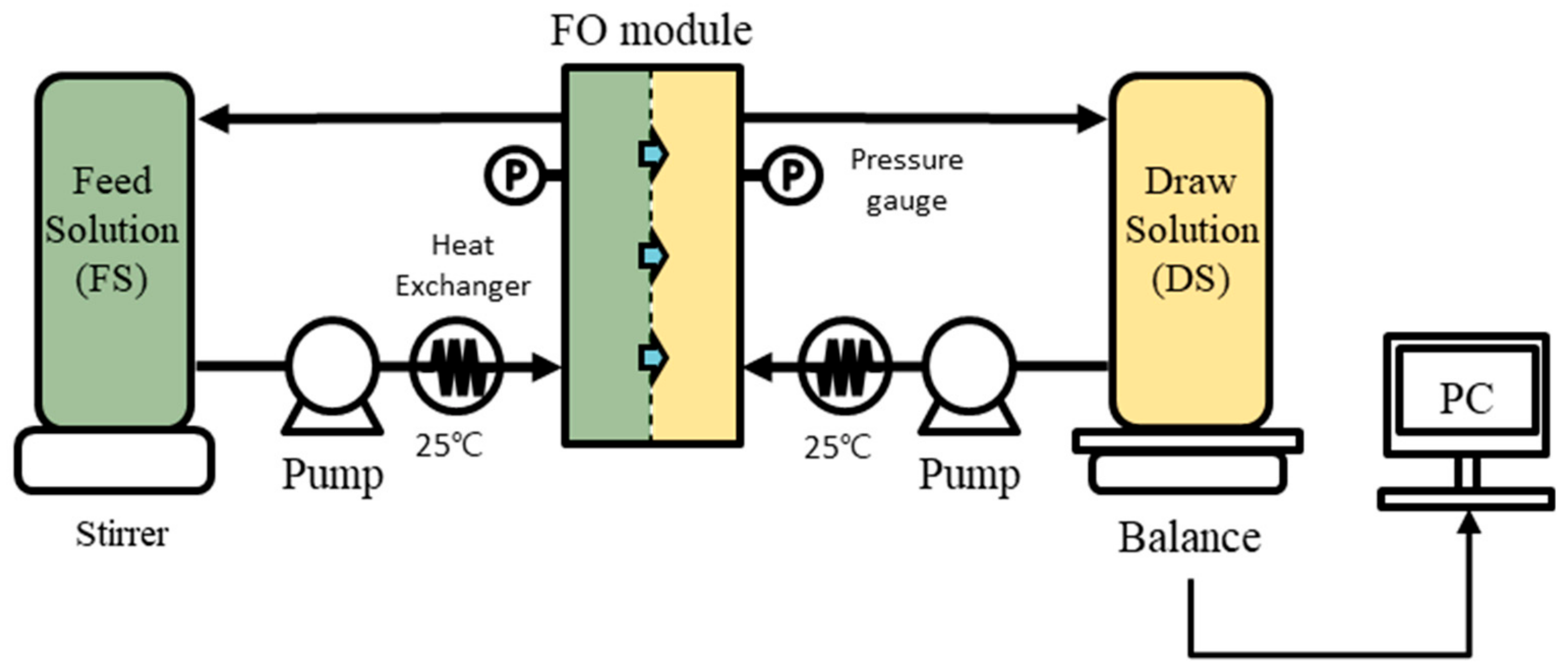
In this study, a more practical and precise model was developed to realize the real-time behavior of the process with a viral equation, represented by concentrations, volumes, and water flux of the system. The model parameters were estimated to reflect the effects of high concentrations of glucose as draw solute. To validate the proposed model, FO filtration experiments were carried out with a commercialized FO membrane in batch mode using glucose as a draw solute and deionized water and glucose solution as a feed solution. For the batch operation of the FO process, the model prediction of the permeate flux profiles was found to be in line with the experimental data. To obtain insight into the dominant factors affecting permeate water flux, global sensitivity analysis using the Latin-hypercube—one-factor-at-a-time (LH—OAT) method was carried out.

2. Modeling Procedures

2.1. Water Flux in Forward Osmosis Process

The transport of water molecules through FO membranes can be represented by irreversible thermodynamics, with the membrane treated as a black box, as has been done for biological membranes [24]. In this approach, the water flux ( J w ) for the FO process (
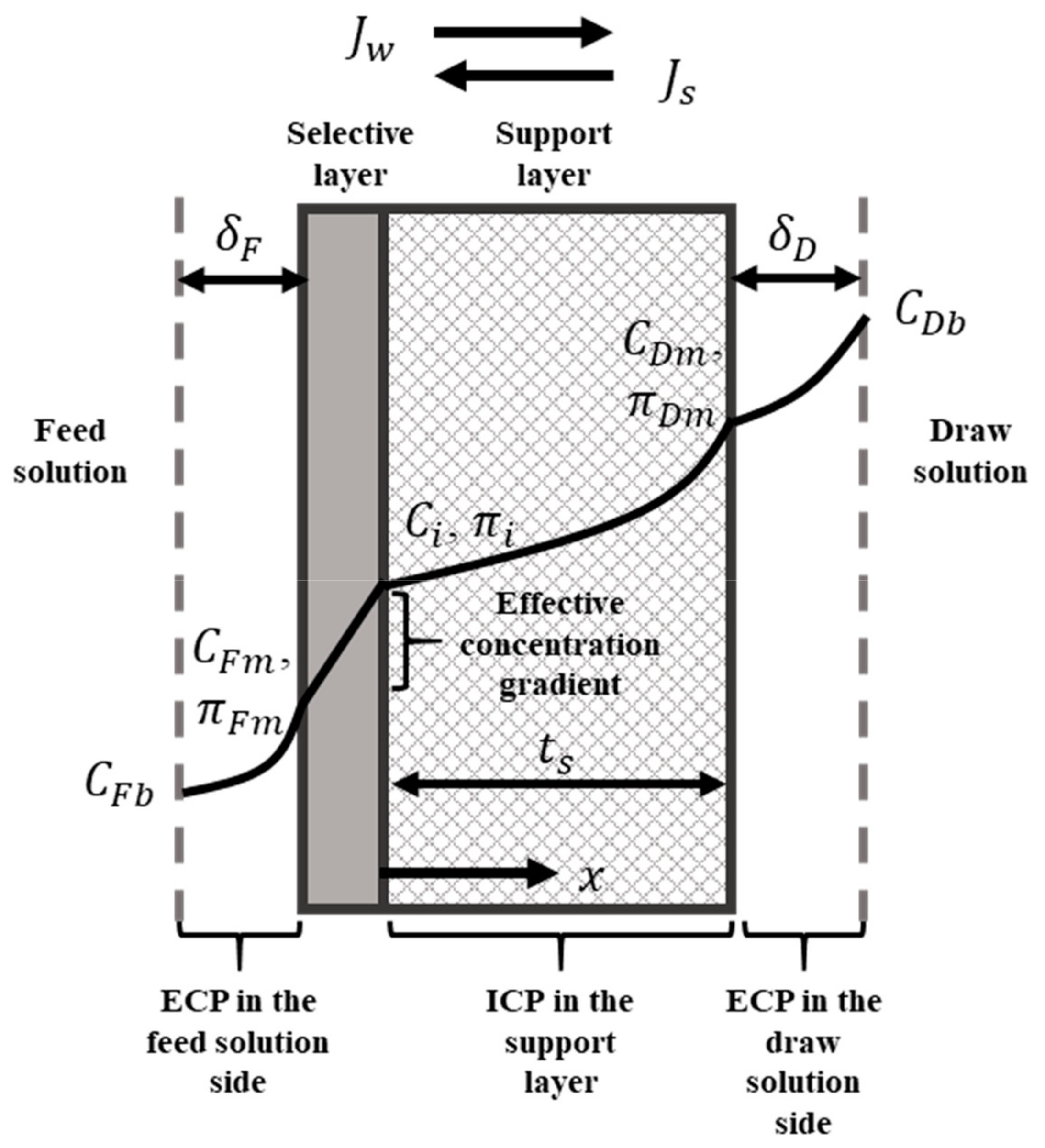
Figure 1), in which hydraulic pressure differences are absent, can generally be described as follows,
J w = A π i   π F m
where A is the water permeability, π i represents the osmotic pressure at the interface between selective layer and support layer, and π F m represents the osmotic pressure at the interface between selective layer and feed solution as shown in Figure 1. This equation indicates that the water flux is linearly proportional to the effective osmotic pressure difference, π i   π F m , across the FO membrane selective layer.

2.2. Osmotic Pressure of Glucose

To establish the relationship between osmotic pressure and solute concentration, the van’t Hoff (1887) equation can be applied for the osmotic pressure ( π ) for an ideal dilute solution [25], that is,
π = n C R T
where n represents the van’t Hoff factor (n = 1 for glucose), C is the solution molar concentration (molarity), R = 0.0821 L·atm·mol−1·K−1 the ideal gas constant, and T is absolute solution temperature (K). Although the van’t Hoff equation is well fitted for dilute and ideal solutions in which ions do not affect each other, this is not applicable to the FO process, which deals with highly concentrated draw and feed solutions [25]. In order to more precisely model the osmotic pressure of general solutions, a modification is made in the van’t Hoff equation, which is then expressed by a virial expansion to a power series [26,27], as follows:
π   = M w 1 c R T   +   B 1 c 2 R T   +   B 2 c 3 R T +   B 3 c 4 R T  
In this equation, the value c represents the solution concentration (g·L−1), Mw is the solute molecular weight, and B1, B2, and B3 are virial osmotic coefficients. It is possible to obtain these virial coefficients empirically by using Equation (3) to fit the experimental osmotic pressure data. It is generally accepted that it is sufficient to determine the coefficients up to the second coefficient (B1 and B2) for the purpose of reproducing the observed osmotic pressure [28].

2.3. Concentration Polarization

Many experimental and theoretical studies have demonstrated that observed water flux values are significantly smaller than those calculated on the basis of difference in bulk concentration. The reason behind this discrepancy is the formation of ICP and ECP; both decrease the effective concentration slope across the FO membrane selective layer; as a result, the value of water flux that is observed, J w , is inevitably lower than expected [29].

2.3.1. Internal Concentration Polarization

It is known that ICP in the support layer can cause severe degradation of cross-membrane water permeation in the FO process [17]. For a porous support layer, in which draw solution is in contact with the porous support, there is a concentration gradient that is steeper than that found in bulk solution. This happens because of decreased solute diffusivity due to porosity and tortuosity. This dilutive ICP brings about a decrease in the net concentration difference across the selective layer and results in a corresponding decline in water flux [29]. According to previous studies [14,23], the solute concentration at the interface between support and selective layers ( C i ) can be described as follows:
C i = C D m exp J w t s D s J s J w 1 exp J w t s D s = C D m exp J w S D J s J w 1 exp J w S D .
Here, C D m represents the concentration of the solute on the surface of the support layer membrane and t s indicates thickness of the support layer D s is the reduced solute diffusivity in the porous support layer [30]. S denotes the membrane structural parameter of the support layer, described as follows [14],
S = t s τ ε  
Equation (5) pertains to the effective distance of the support layer through which a solute must pass to move to the selective layer from the boundary area of the support layer and the draw solution. In experiments using both RO and FO, the average distance of S can be determined and has been described in the literature [14].

2.3.2. External Concentration Polarization

ECP is of great importance in any pressure-driven desalination process, e.g., reverse osmosis [31]. This holds true for the FO system, as the presence of ECP lowers the water movement via a reduced effective concentration gradient through the membrane. This phenomenon was reflected even in some early FO models, such as those of Phillip [14] and Suh and Lee [23]. In fact, because the FO membrane is in contact with two different solutions, ECP can arise on both sides of the membrane surface. To elaborate, the feed side membrane surface faces a concentrated feed solution, a phenomenon termed concentrative ECP; the permeate side membrane surface faces a diluted solution, a phenomenon termed dilutive ECP. According to previous studies [14,23], the solute concentrations at the membrane surface on the support layer ( C D m ) and selective layer ( C F m ) can be estimated as follows,
C D m = C D b exp J w δ D D   J s J w 1 exp J w δ D D ,
C F m =   C F b exp J w δ F D +   J s J w exp J w δ F D 1 .
Here, C D b and C F b are the bulk solute concentration of draw and feed solutions, respectively. D δ can be described in relation to mass transfer coefficient (k); this value has a direct relationship to the Sherwood number (Sh), and also corresponds to the hydrodynamics of the system ( d h ), which can be estimated in the previous studies [14,19,23,31].

2.4. Reverse Solute Flux (RSF)

J s can also be described as shown below [16]:
J s = B C i C F m .
Here, B is the salt permeation coefficient. Substituting Equations (4) and (7) for C i and C F m into Equation (8) can represent the effective solute flux existing between the draw solution and the feed solution, with measurable variables,
J s = B C D b + J s J w exp J w S D exp J w δ D D C F b + J s J w exp J w δ F D .
Note that Equation (9) contains the proportion of RSF to water flux J s / J w as a repetitive term, referred to as the specific RSF [32]. Past research has demonstrated that the specific value of RSF ( J s / J w ) can be replaced by a constant [14,27,33], meaning that more water flux leads to more draw solute moving through the membrane. Philip et al. [14] and Suh and Lee [23] also dealt with the selectivity of reverse flux ( J w / J s ), which is designated as the reverse form of the specific value of RSF; they also validated the dependency of the reverse flux selectivity ( J w / J s ) on the characteristics of the membrane selective layer (water (A) and solute (B) permeability values in the Appendix A), as follows:
J w J s A B n R T .
This result provides insight into the selectivity of the reverse flux, showing that it is independent of the concentration of the bulk draw solute, the crossflow velocity, and structural parameter S, and can be handled as a constant coefficient determined in experiments, provided that these experiments are conducted with the same membrane, the same draw solutes, and identical temperature. Thus, the specific RSF ( J s / J w ) can be described as a constant model parameter:
J s w = J s J w .
Finally, the equation of reverse solute flux and forward water flux for the FO system can be rearranged as follows:
J w = A n R T C i 1 + B 1 C i + B 2 C i 2 C F m 1 + B 1 C F m + B 2 C F m 2 .
It should be noted that for Equation (12), C D b and C F b are easily measurable independent variables, and A, D , S , and J s w are model parameters. Before simulating FO performance, these model parameters should be determined by experiments. Then, only one unknown dependent variable of the equation remains, namely J w . However, Equation (12) is implicit forms with regard to J w , and cannot be solved explicitly. Consequently, recursive numerical procedures must be used to solve these implicit flux equations.

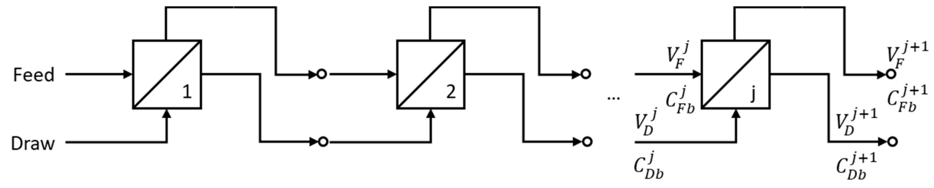
2.5. Mass Balance for Dynamic Modeling (Multistage Operation)

When FO is carried out as a batch operation in such a way that there is an increase of the draw volume and a decrease of the feed volume, such that water molecules continually traverse the FO membrane from feed solution to draw solution, as shown in Figure 2, the time profile for the entire system changes analogously depending on the actual time and can, if the observation time interval (or sampling time interval) of each stage is sufficiently short but not too short (because mass transfer should be reached in quasi-steady state), be expressed as a discrete multistage process, as shown in Figure 3. Considering module length and average crossflow velocity of solution, we set the observation time interval or sampling time interval to 0.5 s because the water molecule takes 0.5 s after entering to exit the FO module. It is assumed that the FO system reaches quasi-steady state at each stage during this sampling time interval. The mass balance of solutes for feed and draw solutions at the j-th stage (or at the j-th sampling in Figure 3) of the FO unit for batch operation can be represented by
C D b j + 1 V D j + 1 = C D b j V D j   J S j t s A m
and
C F b j + 1 V F j + 1 = C F b j V F j   J S j t s A m .
Here, C represents the concentration of individual components, V is the volume, Js is the reverse solute flux, Am is the effective area of the membrane, ts is the time interval, the subscript Fb is the bulk feed solution, the subscript Db is the bulk draw solution, the subscript D is the draw solution, the subscript F is the feed solution, and the superscript j is the sampling index.
The total volume of the system, including the feed and draw solutions, remains constant because the volume loss of the feed solution via transverse-FO-membrane water flux permeation is included in the draw solution volume. This relationship is presented below.
V D j + 1 = V D j   +   J w j t s A m
and
V F j + 1 = V F j   +   J w j t s A m .
Here, Jw is forward water flux.

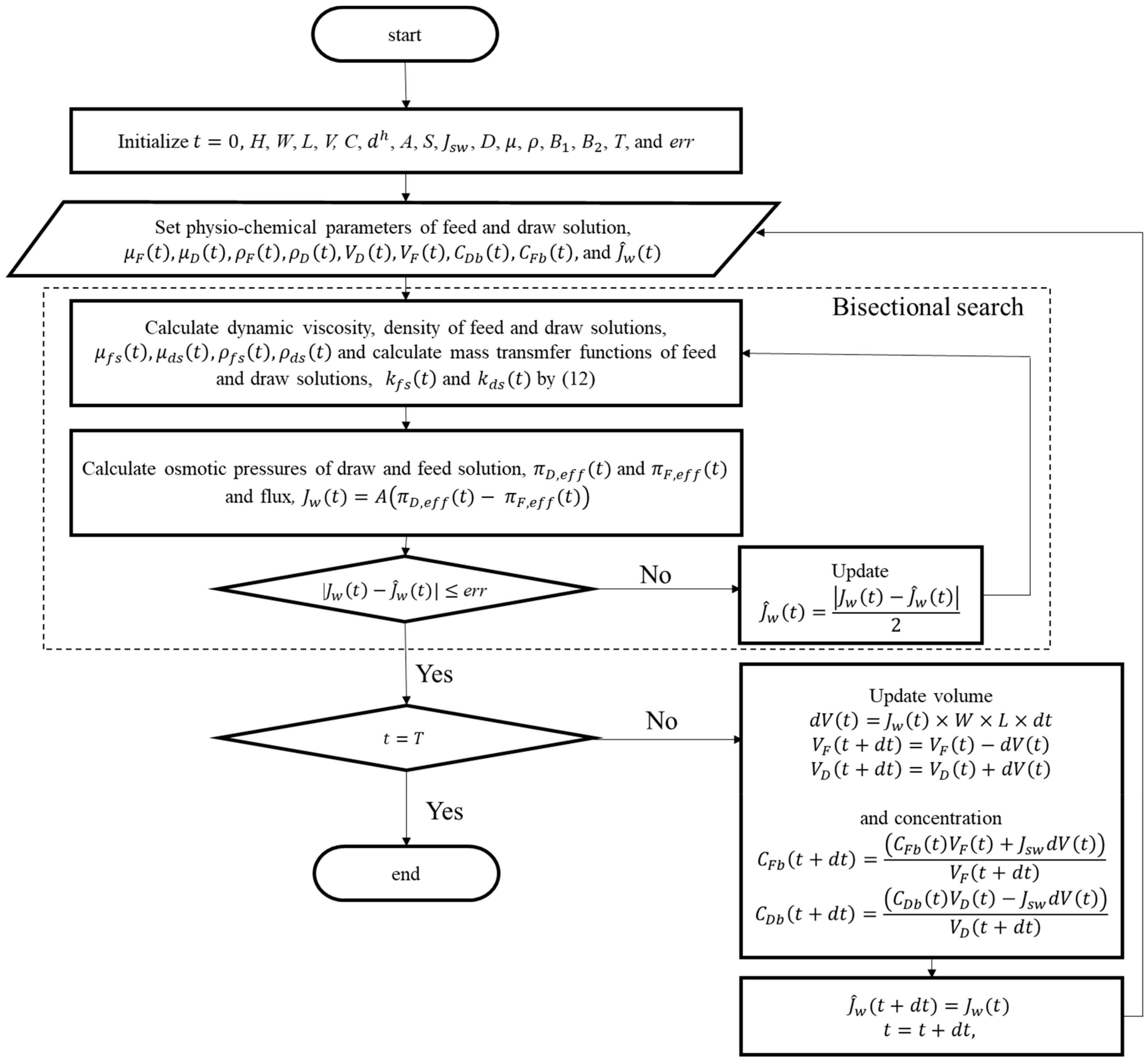
2.6. Numerical Simulations

Using the proposed model for the FO process, all iterative calculations for the water flux profile were conducted with MATLAB software under conditions identical to those of the batch operation experiments described above. Figure 4 provides a flow chart of the proposed multistage FO modeling procedure. First, the timer was reset, and invariant variables were initialized. Then, the initial physio-chemical parameters of the feed and draw solutions of the j-th stage are set. In this step, the initial estimate of water flux j ^ w t was also properly set. With the given physio-chemical variables and j ^ w t , calculations of the dynamic viscosity, density, and mass transfer functions of the feed solution and the draw solution were performed, yielding feed and draw solution osmotic pressure values. From the obtained osmotic pressures, the water flux J w t was obtained. This calculation was repeated with the updated J ^ w t using the mean value of J ^ w t and J w t until the error tolerance condition, J w t J ^ w t e r r , was satisfied. The implicit equation in the proposed model was solved using the bisectional method: The embedded MATLAB ‘fzero’ function [23]. If this j-stage is not reached by the final stage, as we had hoped, i.e., t = T , the volume and feed and draw solution concentrations were revised using the value of J w t determined for the next stage.

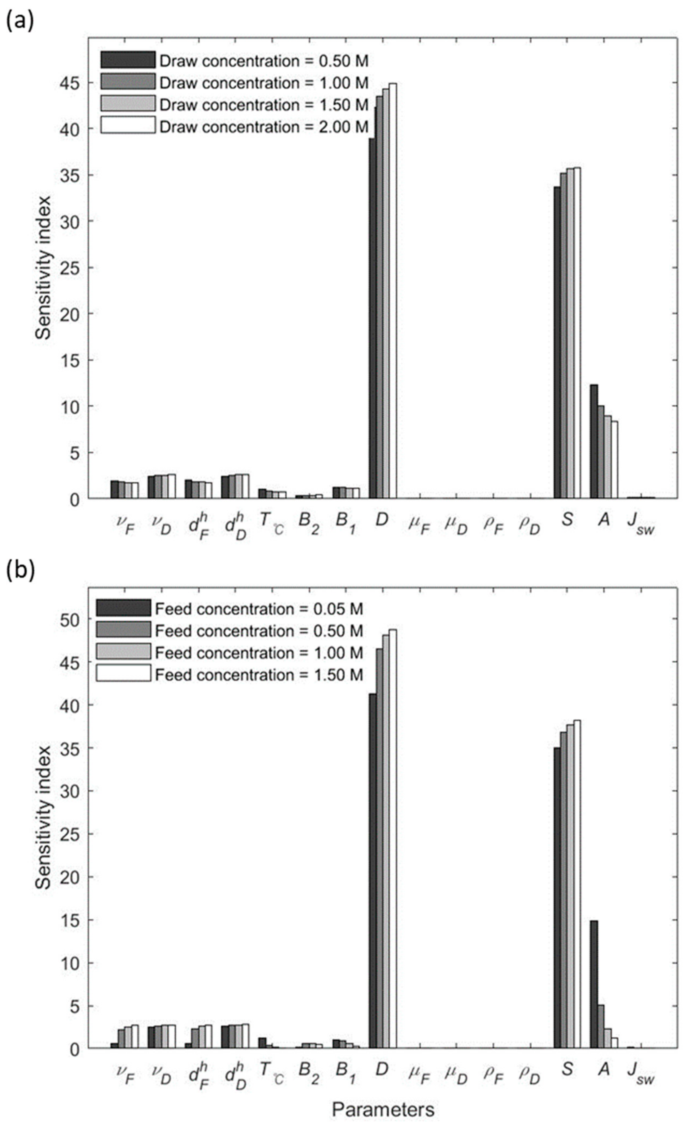
2.7. Sensitivity Analysis Using Latin-Hypercube—One-Factor-at-a-Time (LH–OAT) Method

Sensitivity analyses of model parameters and operating conditions were executed with the Latin-hypercube—one-factor-at-a-time (LH–OAT) method [34], combing Latin-hypercube (LH) sampling [35] and one-factor-at-a-time methods (OAT) [36]. In the LH method, proposed by McKay for use instead of the Monte Carlo method, the parameter space is divided into N intervals with the same probability, and only one variable is randomly extracted from each interval and analyzed by multivariate linear regression. Though this method is advantageous compared to other global sensitivity analyses in that its computational calculation is efficient [34,37], it has limitations in that a linear regression analysis is assumed and the sensitivity to one specific individual variable cannot be identified [34]. To analyze the sensitivity in the OAT method, on the other hand, only one variable in the parameter space is sequentially selected for a small change of the selected parameter, while other parameters are fixed as constant [36,38]. In general, the OAT method has been widely used as an efficient method of local sensitivity analysis. One downside is that it does not give any information on global sensitivity for the whole parameter space. By combining LH sampling and OAT design, therefore, the merits of both methods can be exploited [39]. The process begins with sampling N LH points randomly for N intervals as initial points; this is followed by OAT analysis, in which each of the P parameters is changed [34]. For sensitivity analysis, parameters affecting FO performance were investigated by changing figures with standard deviations of 10%.
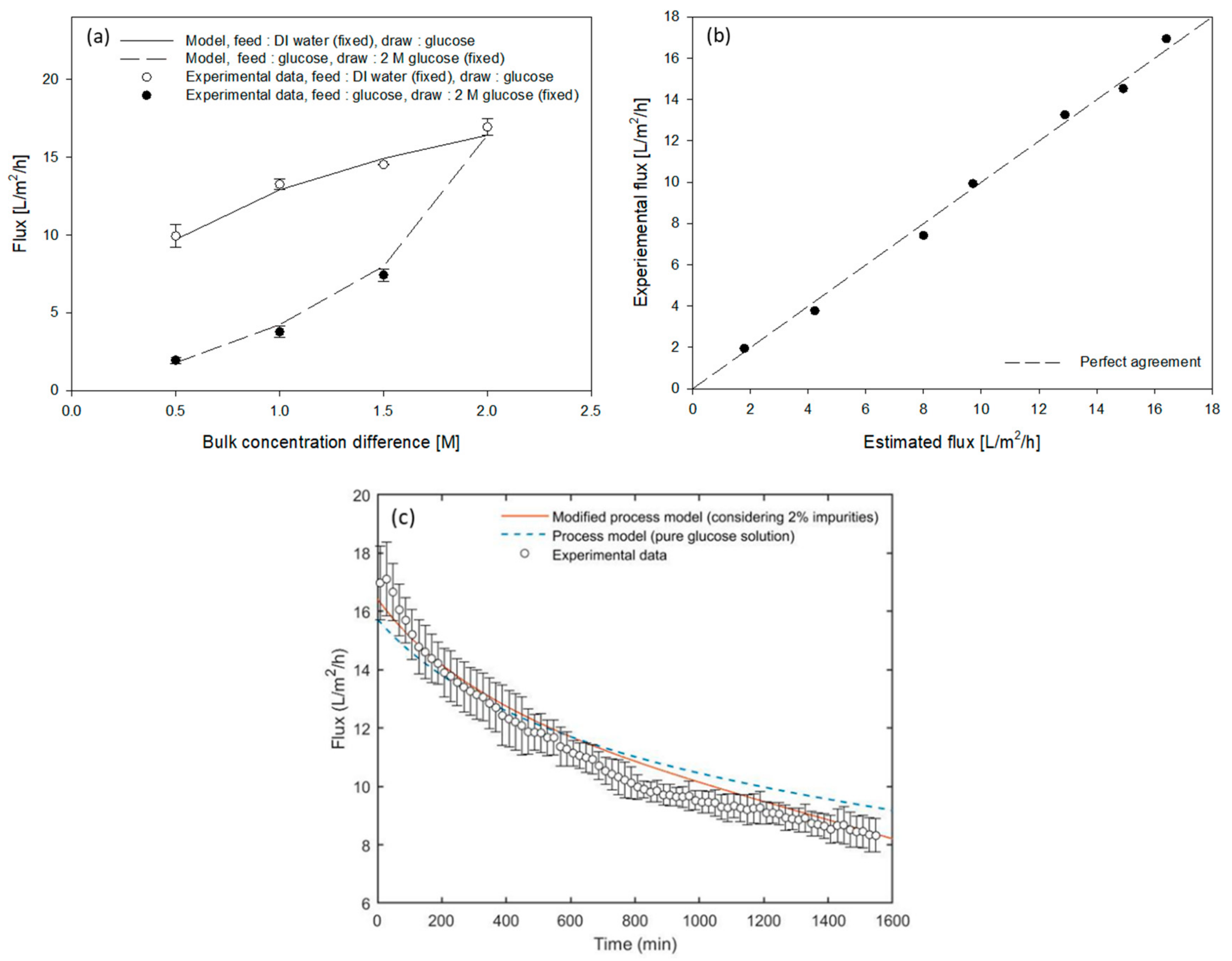
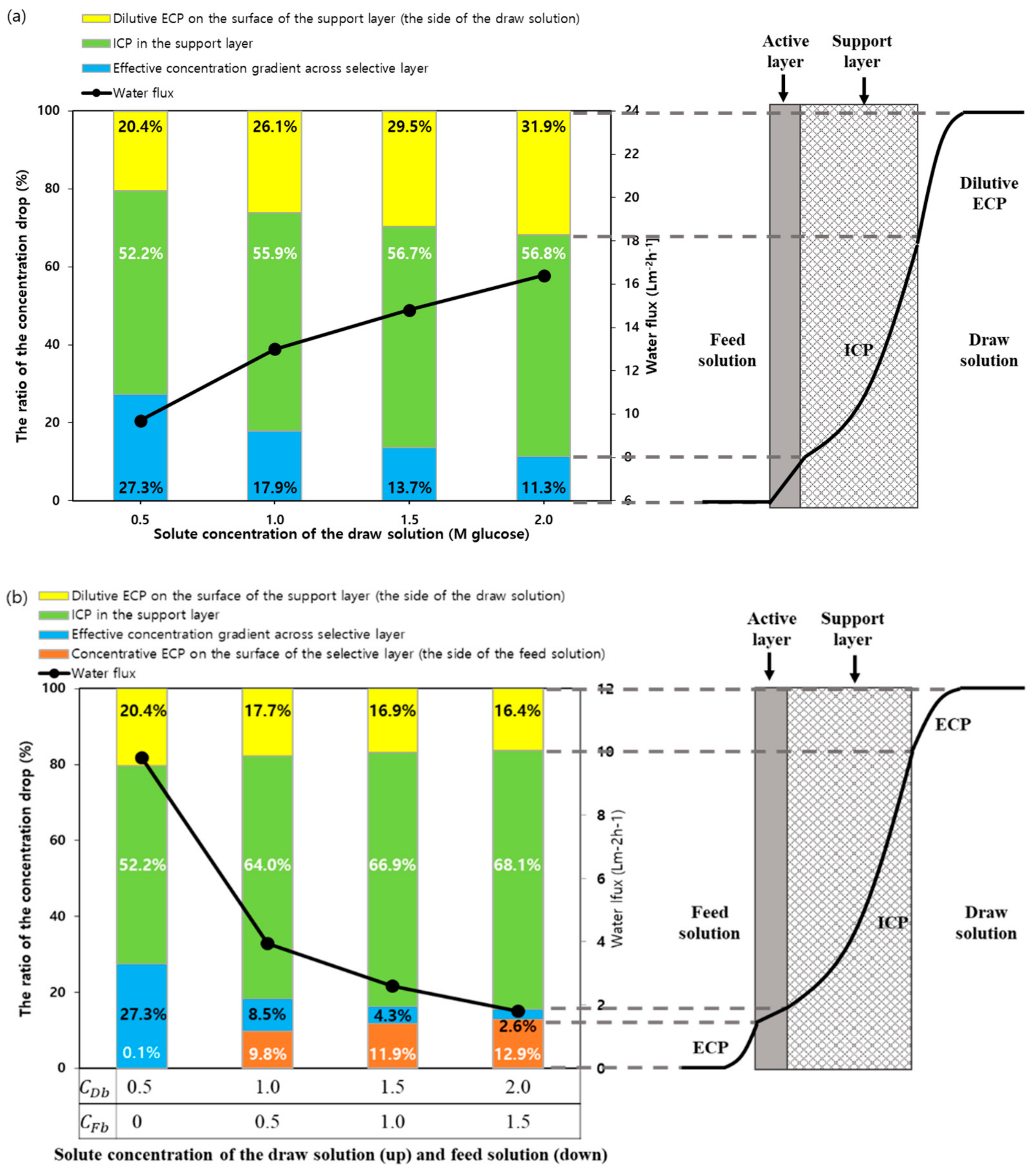
3. Materials and Methods

3.1. Preparation of Feed and Draw Solution

ACS grade glucose (Daejung Chemicals and Metals Co. Ltd., Busan, Korea), which is neutral and highly soluble in water, was utilized as a draw solute. For all empirical procedures, glucose was dissolved in deionized (DI) water (Merck, Daejeon, Korea), which has a resistance value of 18.2 MΩcm at concentrations in the range of 0 to 2.0 M. Viscosity and osmotic pressures for each concentration were measured using a viscosity meter, SV-10 (A&D, Seoul, Korea) and an osmometer, Osmomat 0300-D (Gonotec, Berlin, Germany), respectively. Binary bulk diffusion coefficients for glucose and DI water were maintained at a constant value   ( 6.7 × 10 10 m2/s) [40,41]. The density of each glucose solution was calculated using the Aspen HYSYS® (Cambridge, MA, USA) chemical database. The characteristics of glucose solutions are summarized in Table 1.

3.2. Membrane Preparation and Crossflow Setup

A commercial thin-film composite (TFC) membrane (Porifera, Hayward, CA, USA), known for use in osmotically driven processes, was employed for the FO experiments. This membrane, which has a flat-sheet form, has an asymmetric structure of porous support layer and dense selective layer. This membrane has seen wide use in past research [42,43,44]. Referring to previous studies [42,43], the intrinsic performance parameters of the membrane are summarized in Table 2. The purchased membrane was preserved in DI water at a temperature of 4 °C and was rinsed with DI water prior to use.
A widely used bench-scale FO set up was constructed and used to estimate the permeated water flux [11]. The crossflow membrane unit (2.6 cm width × 0.9 cm length × 0.3 cm depth) consisted of an FO cell with channels present on the two membrane sides to promote the flow of feed and draw solutions. As can be seen in Figure 2, the feed solution moved into and out of the feed chamber via a gear pump (Cole-Parmer, Daejeon, Korea). Simultaneously, the draw solution presents in the reservoir circulated into the draw chamber via the same type of pump. Directions of the flow of feed solution and draw solution in the FO module were co-current. The flow rate was maintained at 1.5 L/min by use of a flow meter OM006 (Corea Flow, Daejeon, Korea). The temperature was maintained at 25 ± 1 °C using a heat exchanger (Thermo Fisher, Seoul, Korea A) with a constant-temperature bath. The resulting permeate water flowing through the FO membrane was quantified using a computer-linked analytical balance (CAS, Daejeon, Korea). Operating conditions for simulations and experiments are summarized in Table 3.

3.3. Forward Osmosis Runs for Model Validation

After the membrane was loaded into the unit module with FO mode orientation, the FO system was first operated using deionized water for the feed and draw solutions for 0.5 h; this was done to achieve temperature equilibrium and operational stabilization. Then, to achieve the necessary concentration, a designated quantity of stock glucose solution (4 M) was put into the draw solution tank; the permeated water flux was then quantified. After measuring the water flux, a certain amount of glucose stock solution was put into the draw solution tank to establish the next desired concentration. The aforementioned procedure was continued in a consecutive manner to draw solution concentrations of 0.5, 1, 1.5, and 2 M glucose. After measuring the flux for the last and highest concentration (i.e., 2 M) with a feed solution of DI water, a certain amount of the stock 4 M glucose solution was put into the feed solution to obtain the required feed solution concentration. Flux was measured at 0.5, 1.0, and 1.5 M concentrations of glucose with the draw solution concentration fixed at 2.0 M.

4. Results and Discussion

4.1. Parameter Estimation

Among the model parameters, the following physiochemical properties of the glucose solution were explored: Osmotic pressure ( π ) , viscosity ( μ ), and density ρ . As shown in Figure 5a, the osmotic pressure of the glucose solution, which was measured experimentally using an osmometer, was different from that obtained by van’t Hoff equation calculation in the region of the high glucose concentration. A more precise prediction can be achieved by means of a virial equation using a power series, as shown Equation (3). Using the second-order polynomial regression of π c R T and the glucose concentration, the virial coefficients B1 and B2 in Equation (3) can be estimated from the experimental osmotic pressure measured at different glucose concentrations, as shown in Figure 5b and Table 1. The viscosity of the solution affects the mass transfer during filtration. The decreased mass transfer rate due to the high viscosity aggravates ECP and thereby ends in a reduction of the water flux. Using a second-order polynomial regression, the viscosity ( μ ) of the glucose solution can be empirically shown to be a function of the molar concentration (C), as shown in Figure 5c and Table 1. Their relationship can be obtained as follows, in which the coefficients are obtained by the second-order polynomial regression
μ = 8.60 × 10 1 +   2.58 × 10 1 C + 4.63 × 10 1 C 2 .
According to data sourced from the Aspen HYSYS® (Cambridge, MA, USA) chemical database, the density ( ρ ) of the glucose solution also increased slightly in line with its molar concentration (C). This relationship can be expressed as shown below for which the coefficients are obtained by a second-order polynomial regression
ρ = 997.1679 +   27.0967 C + 3.6 × 10 4 C 2 .
Among the model parameters, the physio-chemical properties of the FO membrane (Porifera, USA) have been thoroughly studied, with several reports in the literature [42,43,44] focusing on the following: The water permeability (A), the structural parameter (S), and the specific reverse solute (glucose) flux ( J s w ) of the membrane. The water permeability and structural parameter were sourced from the literature [43]. The specific reverse solute (glucose) permeability of the membrane J s w was found in another work [42]. These physiochemical properties of FO are summarized in Table 2.

4.2. Model Verification

Figure 6 shows the model verification process, which relied on comparisons of predicted data obtained using the proposed model and experimental data obtained under identical conditions for FO operations in the FO mode orientation described above. Water flux was plotted against the net concentration difference of the bulk feed and glucose draw solutions (Figure 6a). Dilutive ICP and ECP are on the side of the draw solution. The solid line and the white circle indicate the flux; the feed solution is DI water. When concentrative ECP, dilutive ECP, and ICP are present, the dashed line and black circle show the flux, with glucose solution as the feed. The model predictions of the flux, depicted as solid and dashed lines, agreed well with the empirical results, depicted as white and black circles. More specifically, the experimental flux data were plotted against the data for the estimated flux shown in Figure 6b. The slope of this relationship lies near the dashed line (slope = 1), which means that the model predictions and the experimental results are in perfect agreement. The mean squared error (MSE) between the predicted water flux and the experimental flux data is 0.09, and the R-squared value (R2) is 0.99.
The water flux profiles for the batch operation plotted against time are shown in Figure 6c. The blue dashed line represents the process model flux; this is based on the assumption that the glucose solute used is 100% pure. The model prediction of the water flux, represented as the blue dashed line in Figure 6c, initially agreed to a moderate degree, within ±1.0%, with the empirical data; however, over time, this value diverged from the experimental data. This unexpected discrepancy might be due to impurities that were actually contained (around 2%) in the supposedly pure chemical; worse yet, all compounds were ionic compounds, which was not taken into consideration in the modeling process. There is the possibility that the unknown compounds diffused from the draw solution to the feed solution and as a result, were able to build up, in a gradual manner, in the feed solution, impacting considerably the net driving concentration gradient. It is not uncommon that FO models pay too little attention to impurities, and rightly so, seeing that the primary goal is to obtain values for the instantaneous water flux or initial water flux of the FO system, and not the flux change over time. In this study, the 2% impurities were treated as an ionic pure chemical of NaCl, and their behavior was reflected in the modified process model. With the properties of NaCl as listed in Table 4, the modified process model can be depicted by the red solid line in Figure 6c. The modified model prediction of water flux showed better fit to the experimental data than did the unmodified model prediction. All of this demonstrates that the model precisely represents the practical mass transfer phenomenon occurring in the FO membranes.

4.3. Effects of Changes in the Concentration Difference on Concentration Polarization

The developed FO model was used to investigate how changes in the bulk concentration differences influence the concentration polarization and water flux. Using deionized water as a feed solution and glucose as a draw solution, with concentrations in the range of 0.5 to 2.0 M, Figure 7 shows the proportion of each concentration polarization and resultant water flux. All model conditions were identical to those in the previous parameter estimation and model validation. The side view of Figure 7a shows a profile of solution concentration change across the membrane when 2 M glucose is used for the draw solution; it can be interpreted that the water flux increment was reduced as the draw solution concentration increased. The percentage of effective concentration difference for water transfer across the selective layer decreased from 27.3% to 11.3% when the concentration of the draw solution was increased; on the other hand, the proportions of dilutive ICP and ECP increased. The decline in the increase of the slope of the water flux can be explained in terms of the comparatively increased ratio of ECP on the support layer surface and support layer ICP.
The most likely reason behind the driving force reduction is probably the presence of internal ICP [22,29,45]. In addition, the ratio of ICP increased from 52.2% to 56.8% with the increase of the draw solution concentration shown in Figure 7a. Surprisingly, there was a significant increment of the dilutive ECP in the draw solution side boundary layer; the increase was in the range of 20.4% to 31.9% as the solute concentration of the draw solution increased. Dilutive ECP may have a crucial role under certain circumstances, e.g., when a mixed solution is applied and/or when low crossflow velocities or high water flux levels are used [46,47]. However, the effect of ECP in a concentrative form on the side of the feed solution, with deionized water as a feed solution, was found to be insignificant for all conditions of the draw solution concentration because the simulation also clearly revealed that the concentrative ECP decreased from 0.07% to 0.03%, which is not shown in Figure 7.
Figure 7b shows the ratio of each concentration polarization and resultant water flux when the concentration difference of the bulk solution was maintained at 0.5 M glucose across the membrane, with a range of different feed solute concentrations (0, 0.5, 1, and 1.5 M glucose) and draw solution concentrations (0.5, 1, 1.5, and 2 M glucose). By maintaining the net concentration gradient of the bulk solution, this simulation attempted to discern the effects of the utilized non-dilute feed and draw solutions. All other conditions were identical to those in the previous simulation. The side view of Figure 7b shows the concentration change profile of the solution across the membrane with 1.5 and 2.0 M glucose solutions as the feed and draw solutions, respectively.
As presented in Figure 7b, when the concentration of the feed solution surpasses a certain level, the ratio of the concentrative ECP increased from 0.1% to 12.9% under the condition of the ideal net concentration difference in bulk phase, which implies that the concentrative ECP should not be assumed to have little influence on the water flux; rather, it is because the absolute concentrations of the two solutions, both the feed and the draw, was increased. Furthermore, the ICP was increased from 52.2% to 68.1% when the draw solution concentration was increased from 0.5 to 2.0 M, suggesting that the concentration of the draw solution has a direct effect on the severity of the ICP. Resultantly, both processes end up slowing down the diffusional movement of water molecules. When the feed solution is highly concentrated, the draw solution concentration has to be correspondingly high in order for water permeation to take place, all because of natural osmotic pressure. However, Figure 7b reveals that the high salinity of both solutions worsens the level of ICP and concentrative ECP. This result is consistent with the results of previous studies involving NaCl as a draw solution [23].

4.4. Sensitivity Analysis

In the proposed model, parameters that can possibly affect the permeated water flux can be categorized into operating conditions, membrane properties, and solution properties, as listed in Table 1, Table 2 and Table 3. In this study, the bulk diffusion coefficient of glucose (D), the first and second virial coefficients (B1 and B2), the viscosities of the feed and draw solutions ( μ F and μ D ), the densities of the feed and draw solutions ( ρ F and ρ D ), the water permeability (A), the structural parameter (S), the specific reverse solute flux for glucose ( J s w ), the linear velocities of the feed and draw solutions ( ν F and ν D ), the hydraulic diameters of the feed and draw channels ( d F h and d D h ), and the system temperature ( T ) were selected for the sensitivity analysis. This sensitivity analysis was meant to provide relative and quantified indices of influential factors and thereby insight into the characteristics of the FO process.
Figure 8 shows the sensitivity indices of the 15 parameters under different conditions. Similar to previous studies [23,48], four different feed concentrations, for which the glucose concentration of the draw solution varies from 0.5 to 2.0 M while maintaining the 0.25 M glucose concentration of the feed solution, were applied while the draw concentration was kept constant at 2.0 M (Figure 8a), and four different draw concentrations were used when the feed concentration was fixed at 0.25 M (Figure 7b). Under all different combinations of the feed and draw concentrations, the diffusivity of the draw solute (D) had the highest sensitivity index, followed by S and A. An increase of S negatively affects the permeated water flux, while increases in D and A positively improve it. Similarly, because D over S ( D S ) is closely tied to the solute mass transfer in the support layer, as described in Equation (4), this value can have a dominant effect on the ICP; that is, an increase of D S alleviates the ICP. As discussed above based on the simulation results, the ICP was a dominant hindrance that caused the water flux to drop. Thus, these sensitivity analysis results, showing that D and B are the parameters that have the most influence on the permeated water flux, are indeed in line with previous simulation results and other studies [23,48]. These results prove that not only developing a support layer but also choosing an appropriate draw solute is important when it comes to FO performance.
When either the feed solution concentration was raised while keeping the draw solution fixed, or the draw solution concentration was increased while keeping the feed solution fixed, the sensitivity indices D and S rose while that of A decreased, as shown in Figure 7. As mentioned for the previous simulation, the ICP and ECP have specific effects on the water flux that increase according to the concentrations of the feed and draw solutions, implying that D and B are more related to the ICP and ECP compared to A. Thus, when dealing with high salinity solutions, the augmentation of D S is probably the best method of maximizing the water flux.

5. Conclusions

In this paper, a numerical dynamic model was established, capable of predicting results for a process of forward osmosis (FO). After a parameter estimation process, the model was found to be capable of describing significant physio-chemical phenomena during the FO process, such as the internal (ICP) and external concentration polarization (ECP), as well as diffusion of the reverse draw solute. The proposed model was verified through comparisons with experimental data. The results of our simulation agree well with the empirical data. Furthermore, the influences of the ICP and ECP on the FO system water flux were investigated with different solute concentrations. The simulation results indicate that the influences of the ICP, ECP, and reverse draw solute flux must be taken into account for FO systems. It was also observed that the concentrative ECP on the selective layer surface does not need to be taken into account when deionized water is used as a feed solution. However, the concentrative ECP is not negligible if the salinity of the feed solution exceeds a certain point. Similarly, the high salinity of a draw solution can affect the dilutive ECP on the support layer surface, because the changes in the ECP can have an effect on the support layer dilutive ICP. Furthermore, with the verified model, a global sensitivity analysis was used to consider the effects of certain model parameters on the FO performance. The simulation results confirmed solute diffusivity is the most influential parameter for water flux; the reason is that the solute diffusivity directly affects both ECP and ICP.

Author Contributions

H.R., A.M., E.P., K.K., Y.K.C., and J.-I.H. were involved in the design and perform of the experiment, to the analysis of the results, and to the writing and revising of the manuscript.

Funding

This research was funded by the Advanced Biomass R&D Center (ABC) of Global Frontier Project of Korea, grant number ABC-2010-0029728 and ABC-2011-0031348. The Advanced Biomass R&D Center (ABC) of Global Frontier Project of Korea was funded by the Ministry of Science and ICT.

Conflicts of Interest

The authors declare no conflict of interest. The funders had no role in the design of the study; in the collection, analyses, or interpretation of data; in the writing of the manuscript, or in the decision to publish the results.

Appendix A

Table A1. Abbreviation.
AWater Permeability
A m effective area of membrane
Bsolute permeability
B1first virial coefficient
B2second virial coefficient
Cmolar concentration
cmass concentration
Dbinary bulk diffusion coefficient of solute in water
d h hydraulic diameter
J s reverse solute flux
J s w specific reverse solute flux
J w forward water flux
kmass transfer coefficient
Lchannel length
Mwmolecular weight
nnumber of dissolved species (van’t Hoff factor)
Rideal gas constant
ReReynolds number
Sstructural parameter of support layer
ScSchmidt number
ShSherwood number
Tabsolute Temperature
T temperature in Celsius degree
t s thickness of support layer
v D average crossflow velocity of draw solution
v F linear crossflow of feed solution
Table A2. Symbols.
Table A2. Symbols.
δ Boundary Layer
ε porosity of support layer
μ viscosity of solution
π osmotic pressure
ρ density of solution
τ tortuosity of support layer
Table A3. Subscripts.
bbulk solution
Ddraw solution
Ffeed solution
gluglucose
Iinterface between selective and support layers
mmembrane surface
ssolute
wwater
Table A4. Superscript.
jsampling index

References

  1. Nations, U. The United Nations World Water Development Report; UNESCO: Paris, France, 2019. [Google Scholar]
  2. Shannon, M.A.; Bohn, P.W.; Elimelech, M.; Georgiadis, J.G.; Mariñas, B.J.; Mayes, A.M. Science and technology for water purification in the coming decades. Nature 2008, 452, 301–310. [Google Scholar] [CrossRef] [PubMed]
  3. Monnot, M.; Nguyên, H.T.K.; Laborie, S.; Cabassud, C. Seawater reverse osmosis desalination plant at community-scale: Role of an innovative pretreatment on process performances and intensification. Chem. Eng. Process. Process Intensif. 2017, 113, 42–55. [Google Scholar] [CrossRef]
  4. Al Hawli, B.; Benamor, A.; Hawari, A.A. A hybrid electro-coagulation/forward osmosis system for treatment of produced water. Chem. Eng. Process. Process Intensif. 2019, 143. [Google Scholar] [CrossRef]
  5. Nguyen, T.-T.; Kook, S.; Lee, C.; Field, R.W.; Kim, I.S. Critical flux-based membrane fouling control of forward osmosis: Behavior, sustainability, and reversibility. J. Membr. Sci. 2018, 570, 380–393. [Google Scholar] [CrossRef] [Green Version]
  6. Gulied, M.; Al Momani, F.; Khraisheh, M.; Bhosale, R.; AlNouss, A. Influence of draw solution type and properties on the performance of forward osmosis process: Energy consumption and sustainable water reuse. Chemosphere 2019, 233, 234–244. [Google Scholar] [CrossRef]
  7. Petrotos, K.B.; Quantick, P.; Petropakis, H. A study of the direct osmotic concentration of tomato juice in tubular membrane – module configuration. I. The effect of certain basic process parameters on the process performance. J. Memb. Sci. 1998, 150, 99–110. [Google Scholar] [CrossRef]
  8. Petrotos, K.B.; Quantick, P.C.; Petropakis, H. Direct osmotic concentration of tomato juice in tubular membrane – module configuration. II. The effect of using clarified tomato juice on the process performance. J. Memb. Sci. 1999, 160, 171–177. [Google Scholar] [CrossRef]
  9. Roy, D.; Rahni, M.; Pierre, P.; Yargeau, V. Forward osmosis for the concentration and reuse of process saline wastewater. Chem. Eng. J. 2016, 287, 277–284. [Google Scholar] [CrossRef] [Green Version]
  10. Phuntsho, S.; Shon, H.K.; Majeed, T.; El Saliby, I.; Vigneswaran, S.; Kandasamy, J.; Hong, S.; Lee, S. Blended Fertilizers as Draw Solutions for Fertilizer-Drawn Forward Osmosis Desalination. Environ. Sci. Technol. 2012, 46, 4567–4575. [Google Scholar] [CrossRef]
  11. Chekli, L.; Kim, Y.; Phuntsho, S.; Li, S.; Ghaffour, N.; Leiknes, T.; Shon, H.K. Evaluation of fertilizer-drawn forward osmosis for sustainable agriculture and water reuse in arid regions. J. Environ. Manage. 2017, 187, 137–145. [Google Scholar] [CrossRef] [Green Version]
  12. Zou, S.; He, Z. Enhancing wastewater reuse by forward osmosis with self-diluted commercial fertilizers as draw solutes. Water Res. 2016, 99, 235–243. [Google Scholar] [CrossRef] [PubMed] [Green Version]
  13. Xie, M.; Shon, H.K.; Gray, S.R.; Elimelech, M. Membrane-based processes for wastewater nutrient recovery: Technology, challenges, and future direction. Water Res. 2016, 89, 210–221. [Google Scholar] [CrossRef] [PubMed] [Green Version]
  14. Phillip, W.A.; Yong, J.S.; Elimelech, M. Reverse draw solute permeation in forward osmosis: Modeling and experiments. Environ. Sci. Technol. 2010, 44, 5170–5176. [Google Scholar] [CrossRef] [PubMed]
  15. McCutcheon, J.R.; Elimelech, M. Influence of concentrative and dilutive internal concentration polarization on flux behavior in forward osmosis. J. Memb. Sci. 2006, 284, 237–247. [Google Scholar] [CrossRef]
  16. Lee, K.L.; Baker, R.W.; Lonsdale, H.K. Membranes for power generation by pressure-retarded osmosis. J. Memb. Sci. 1981, 8, 141–171. [Google Scholar] [CrossRef]
  17. Yang, X.; Wang, S.; Hu, B.; Zhang, K.; He, Y. Estimation of concentration polarization in a fluidized bed reactor with Pd-based membranes via CFD approach. J. Memb. Sci. 2019, 262–269. [Google Scholar] [CrossRef]
  18. Touati, K.; Tadeo, F. Study of the Reverse Salt Diffusion in pressure retarded osmosis: Influence on concentration polarization and effect of the operating conditions. Desalin. 2016, 389, 171–186. [Google Scholar] [CrossRef]
  19. She, Q.; Wang, R.; Fane, A.G.; Tang, C.Y. Membrane fouling in osmotically driven membrane processes: A review. J. Memb. Sci. 2016, 499, 201–233. [Google Scholar] [CrossRef]
  20. Hoek, E.M.V.; Kim, A.S.; Elimelech, M. Influence of Crossflow Membrane Filter Geometry and Shear Rate on Colloidal Fouling in Reverse Osmosis and Nanofiltration Separations. Environ. Eng. Sci. 2004, 19, 6. [Google Scholar] [CrossRef] [Green Version]
  21. Loeb, S.; Titelman, L.; Korngold, E.; Freiman, J. Effect of porous support fabric on osmosis through a Loeb-Sourirajan type asymmetric membrane. J. Memb. Sci. 1997, 129, 243–249. [Google Scholar] [CrossRef]
  22. Tang, C.Y.; She, Q.; Lay, W.C.L.; Wang, R.; Fane, A.G. Coupled effects of internal concentration polarization and fouling on flux behavior of forward osmosis membranes during humic acid filtration. J. Memb. Sci. 2010, 354, 123–133. [Google Scholar] [CrossRef]
  23. Suh, C.; Lee, S. Modeling reverse draw solute flux in forward osmosis with external concentration polarization in both sides of the draw and feed solution. J. Memb. Sci. 2013, 427, 365–374. [Google Scholar] [CrossRef]
  24. Kedem, O.; Katchalsky, A. Thermodynamic analysis of the permeability of biological membranes to non-electrolytes. BBA Biochim. Biophys. Acta 1958, 27, 229–246. [Google Scholar] [CrossRef]
  25. Snoeyink, V.L.; Jenkins, D. Water chemistry; John Wiley & Sons Ltd.: Hoboken, NJ, USA, 1980; ISBN 9780471051961. [Google Scholar]
  26. Rudin, A.; Choi, P. The Elements of Polymer Science and Engineering; Elsevier Science: Amsterdam, The Netherlands, 2013. [Google Scholar]
  27. Johnson, D.J.; Suwaileh, W.A.; Mohammed, A.W.; Hilal, N. Osmotic’s potential: An overview of draw solutes for forward osmosis. Desalin 2018, 434, 100–120. [Google Scholar] [CrossRef] [Green Version]
  28. Yokozeki, A. Osmotic pressures studied using a simple equation-of-state and its applications. Appl. Energy 2006, 83, 15–41. [Google Scholar] [CrossRef]
  29. Hsiang Tan, C.; Ng, Y. Modified models to predict flux behavior in forward osmosis in consideration of external and internal concentration polarizations. J. Memb. Sci. 2008, 324, 209–219. [Google Scholar]
  30. Dullien, F.A.L. Porous Media: Fluid Transport and Pore Structure.; Elsevier Science: Amsterdam, The Netherlands, 1991. [Google Scholar]
  31. Mulder, M. Basic Principles of Membrane Technology; Springer: Berlin/Heidelberg, Germany, 1996. [Google Scholar]
  32. Phuntsho, S.; Shon, H.K.; Hong, S.; Lee, S.; Vigneswaran, S. A novel low energy fertilizer driven forward osmosis desalination for direct fertigation: Evaluating the performance of fertilizer draw solutions. J. Memb. Sci. 2011, 375, 172–181. [Google Scholar] [CrossRef]
  33. Tan, C.H.; Ng, H.Y. A novel hybrid forward osmosis - nanofiltration (FO-NF) process for seawater desalination: Draw solution selection and system configuration. Desalin. Water Treat. 2010, 13, 356–361. [Google Scholar] [CrossRef]
  34. Van Griensven, A.; Meixner, T.; Grunwald, S.; Bishop, T.; Diluzio, M.; Srinivasan, R. A global sensitivity analysis tool for the parameters of multi-variable catchment models. J. Hydrol. 2006, 324, 10–23. [Google Scholar] [CrossRef]
  35. Beckman, R.J.; Conover, W.J. A Comparison of Three Methods for selecting Input Variables in the Analysis of Output from a Computer code. Technometrics 2010, 42, 55–61. [Google Scholar]
  36. Morris, M.D. Factorial Sampling Plans for Preliminary Computational Experiments. Technometrics 1991, 33, 161–174. [Google Scholar] [CrossRef]
  37. Jung, Y.W.; Oh, D.-S.; Kim, M.; Park, J.-W. Calibration of LEACHN model using LH-OAT sensitivity analysis. Nutr. Cycl. Agroecosyst. 2010, 87, 261–275. [Google Scholar] [CrossRef]
  38. Huang, J.; Xu, J.; Xia, Z.; Liu, L.; Zhang, Y.; Li, J.; Lan, G.; Qi, Y.; Kamon, M.; Sun, X.; et al. Identification of influential parameters through sensitivity analysis of the TOUGH + Hydrate model using LH-OAT sampling. Mar. Pet. Geol. 2015, 65, 141–156. [Google Scholar] [CrossRef]
  39. Holvoet, K.; van Griensven, A.; Seuntjens, P.; Vanrolleghem, P.A. Sensitivity analysis for hydrology and pesticide supply towards the river in SWAT. Phys. Chem. Earth, Parts A/B/C 2005, 30, 518–526. [Google Scholar] [CrossRef]
  40. Gray, G.T.; McCutcheon, J.R.; Elimelech, M. Internal concentration polarization in forward osmosis: role of membrane orientation. Desalin. 2006, 197, 1–8. [Google Scholar] [CrossRef]
  41. Yong, J.S.; Phillip, W.A.; Elimelech, M. Coupled reverse draw solute permeation and water flux in forward osmosis with neutral draw solutes. J. Memb. Sci. 2012, 392, 9–17. [Google Scholar] [CrossRef]
  42. Kim, D.I.; Choi, J.; Hong, S. Evaluation on suitability of osmotic dewatering through forward osmosis (FO) for xylose concentration. Sep. Purif. Technol. 2018, 191, 225–232. [Google Scholar] [CrossRef]
  43. Gwak, G.; Kim, D.I.; Hong, S. New industrial application of forward osmosis (FO): Precious metal recovery from printed circuit board (PCB) plant wastewater. J. Memb. Sci. 2018, 552, 234–242. [Google Scholar] [CrossRef]
  44. Blandin, G.; Vervoort, H.; Le-Clech, P.; Verliefde, A.R.D. Fouling and cleaning of high permeability forward osmosis membranes. J. Water Process Eng. 2016, 9, 161–169. [Google Scholar] [CrossRef]
  45. Wang, F.; Tarabara, V.V. Coupled effects of colloidal deposition and salt concentration polarization on reverse osmosis membrane performance. J. Memb. Sci. 2007, 293, 111–123. [Google Scholar] [CrossRef]
  46. McCutcheon, J.R.; Elimelech, M. Modeling water flux in forward osmosis: Implications for improved membrane design. AIChE J. 2007, 53, 1736–1744. [Google Scholar] [CrossRef]
  47. Sagiv, A.; Semiat, R. Finite element analysis of forward osmosis process using NaCl solutions. J. Memb. Sci. 2011, 379, 86–96. [Google Scholar] [CrossRef]
  48. Park, P.-K.; Lee, C.-H.; Lee, S. Determination of cake porosity using image analysis in a coagulation–microfiltration system. J. Memb. Sci. 2007, 293, 66–72. [Google Scholar] [CrossRef]
Figure 1. Schematic of flux behaviors and concentration profile for an asymmetric membrane with an orientation of a selective layer that faces the feed solution, or forward osmosis (FO) mode. The internal concentration polarization (ICP) and external concentration polarization (ECP) are considered in the support layer and on both solution sides, respectively. The concentration of the bulk draw solution ( C D b ) is higher than that of the bulk feed solution ( C F b ); this difference in concentration simultaneously creates two opposite directional fluxes: Forward water flux ( J w ) and reverse solute flux ( J s ). With the presence of a concentration gradient, draw solute is diffused into feed solution across the boundary layers ( δ D and δ F ), across the support layer with thickness t s , and across the selective layer. C D m ,   C i , and C F m represent the solute concentrations at the interfaces between (1) the draw solution and the support layer, (2) the support layer and the selective layer, and (3) the selective layer and the feed solution, respectively. π D m , π i , and π F m represent the osmotic pressure of solute concentrations at each interface.
Water 12 00031 g001
Figure 2. Schematic diagram of forward osmosis (FO) system for batch operation.
Water 12 00031 g002
Figure 3. Forward osmosis (FO) system that changes analogously can be expressed as discrete multistage version of the FO model for batch operation. V F j and V D j represents volumes of feed and draw solution, respectively, in the j-th stage. C F b j and C D b j indicates concentrations of feed and draw solution, respectively, in the j-th stage. V F j + 1 and V D j + 1 represent volumes of feed and draw solutions, respectively, in the j+1-th stage. C F b j + 1 and C D b j + 1 represents concentrations of feed and draw solution, respectively, in the j+1-th stage.
Water 12 00031 g003
Figure 4. Flow chart of calculation procedure. MATLAB software was used to solve implicit equations for the given operational conditions.
Water 12 00031 g004
Figure 5. Physio-chemical properties of the glucose solution: (a) Osmotic pressure ( π ) variation with glucose concentration (0.1–1.0 M) at 25 . The white circle represents the osmotic pressure predicted by the van’t Hoff equation. The black circle represents the osmotic pressure measured using an osmometer with the freezing depression method. (b) π c R T plotted as a function of the glucose solute concentration (18.02–180.16 g/L) to determine the osmotic virial coefficients (B1 and B2). (c) The viscosity of the glucose solution plotted as a function of the glucose concentration (0–2.0 M) at 25 . The black square represents the solution viscosity measured using a viscometer (SV-10 VIBRO, Japan). (d) Solution density plotted as a function of the concentration of glucose (0–2.0 M) at 25 . The white triangle represents the solution density calculated using the Aspen HYSYS® (Cambridge, MA, USA) chemical database. Osmotic pressures and viscosities are shown in terms of the mean ± standard deviation, with n = 2.
Water 12 00031 g005
Figure 6. Model validation after comparing the model predictions and water flux empirical results: (a) Solid and dashed lines indicate model predictions; circles indicate empirical data. Using the proposed model and the corresponding physiochemical properties of glucose, as presented in Figure 4, along with the values of the transport parameters from Table 1, the predicted water flux is calculated at 25 ℃ after 5 min. (b) The dashed line (slope = 1) shows excellent agreement between the predictions from the model and the empirical data. The mean squared error (MSE) and R-squared (R2) values are 0.09 and 0.99, respectively. Experimental fluxes are shown in terms of the mean ± standard deviation, with n = 2. (c) Time profile of the water fluxes; under identical experimental conditions, the solid line indicates model prediction and the circles indicate empirical data. Time profiles of experimental fluxes are shown in terms of the mean ± standard deviation, with n = 5.
Water 12 00031 g006
Figure 7. Proportions of the concentration polarization and water flux against the concentration differences of feed and draw solutions based on the simulation results using the proposed model: (a) When a using feed solution of deionized water and draw solutions with various concentrations of glucose (0.5, 1.0, 1.5, and 2.0 M glucose). (b) When the solute concentration difference was held constant, with 0.5 M glucose with various feed solution concentrations (0, 0.5, 1.0, and 1.5 M glucose) and draw solution concentrations (0.5, 1.0, 1.5, and 2.0 M glucose).
Water 12 00031 g007
Figure 8. Sensitivity analysis of the parameters affecting the permeated water flux, obtained using the Latin-hypercube one-factor-at-a-time (LH–OAT) method: (a) Sensitivity indices were simulated by changing the glucose concentration of draw solution from 0.5 to 2.0 M while maintaining the 0.25 M glucose concentration as the feed solution. (b) Sensitivity indices were simulated by changing the glucose concentration in the feed solution from 0.05 to 1.5 M and keeping the 2.0 M glucose concentration of the draw solution. ν is average crossflow velocity, d h is hydraulic diameter of channel, T is temperature ( ) of system, D is diffusivity, μ is solution viscosity, ρ is solution density, S is structural parameter of membrane, A is water permeability of membrane, and J s w is specific reverse solute flux. The subscripts F and D indicate feed solution and draw solution, respectively.
Water 12 00031 g008
Table 1. Model parameters for glucose properties.
ConditionDescriptionUnitValue
D g l u Bulk binary diffusion coefficient of glucosem2·s−1 6.7 × 10 10 (refers to [40,41])
J s w Specific reverse solute flux for glucoseg·L−12.7 × 10 1 (refers to [42])
B11st order virial coefficient- 6.37 × 10 6
B22nd order virial coefficient- 2.16 × 10 8
μ F Feed solution viscositycP 8.60 × 10 1 +   2.58 × 10 1 C + 4.63 × 10 1 C 2
μ D Draw solution viscositycP 8.60 × 10 1 +   2.58 × 10 1 C + 4.63 × 10 1 C 2
ρ F Feed solution densitykg·m−3 997.17 + 27.1 C + 3.6 × 10 4 C 2
ρ D Draw solution densitykg·m−3 997.17 + 27.1 C + 3.6 × 10 4 C 2
Table 2. Model parameters for membrane properties.
ParameterDescriptionUnitValue
AWater permeability coefficientm · Pa−1 · s−1 7.64 × 10 12 (refers to [43])
SStructure parameterm 2.63 × 10 4 (refers to [43])
J sw Specific reverse solute flux for glucoseg · L−12.7 × 10 1 (refers to [44])
J sw Specific reverse solute flux for NaClg · L−14.1 × 10 1 (refers to [44])
Table 3. Operating conditions for simulations and experiments.
ConditionDescriptionUnitValue
d F h Hydraulic diameter of feed channelm 5.4 × 10 3
d D h Hydraulic diameter of draw channelm 5.4 × 10 3
v F Cross-flow velocity of feed solutionm · s−1 3.2 × 10 1
v D Cross-flow velocity of draw solutionm · s−1 3.2 × 10 1
V D Volume of feed solutionL0–2
V F Volume of draw solutionL0–2
C F b Bulk feed concentration (glucose)M0–1.5
C D b Bulk draw concentration (glucose)M0.5–2
TSystem temperature 25
Table 4. Model parameters for NaCl properties.
ConditionDescriptionUnitValue
D N a C l Bulk binary diffusion coefficient of NaClm2·s−1 1.74 × 10 10 (refers to [40,41])
J s w Specific reverse solute flux for NaClg L−14.1 × 10 1 (refers to [23])

