Two-Phase Flow Simulation of Tunnel and Lee-Wake Erosion of Scour below a Submarine Pipeline


Abstract
1. Introduction
2. Materials and Methods
2.1. Governing Equations
2.2. Granular Stress Models
2.2.1. Rheology
2.2.2. Kinetic Theory for Granular Flows
2.3. Turbulence Models
2.3.1. Model
2.3.2. 2006 Model
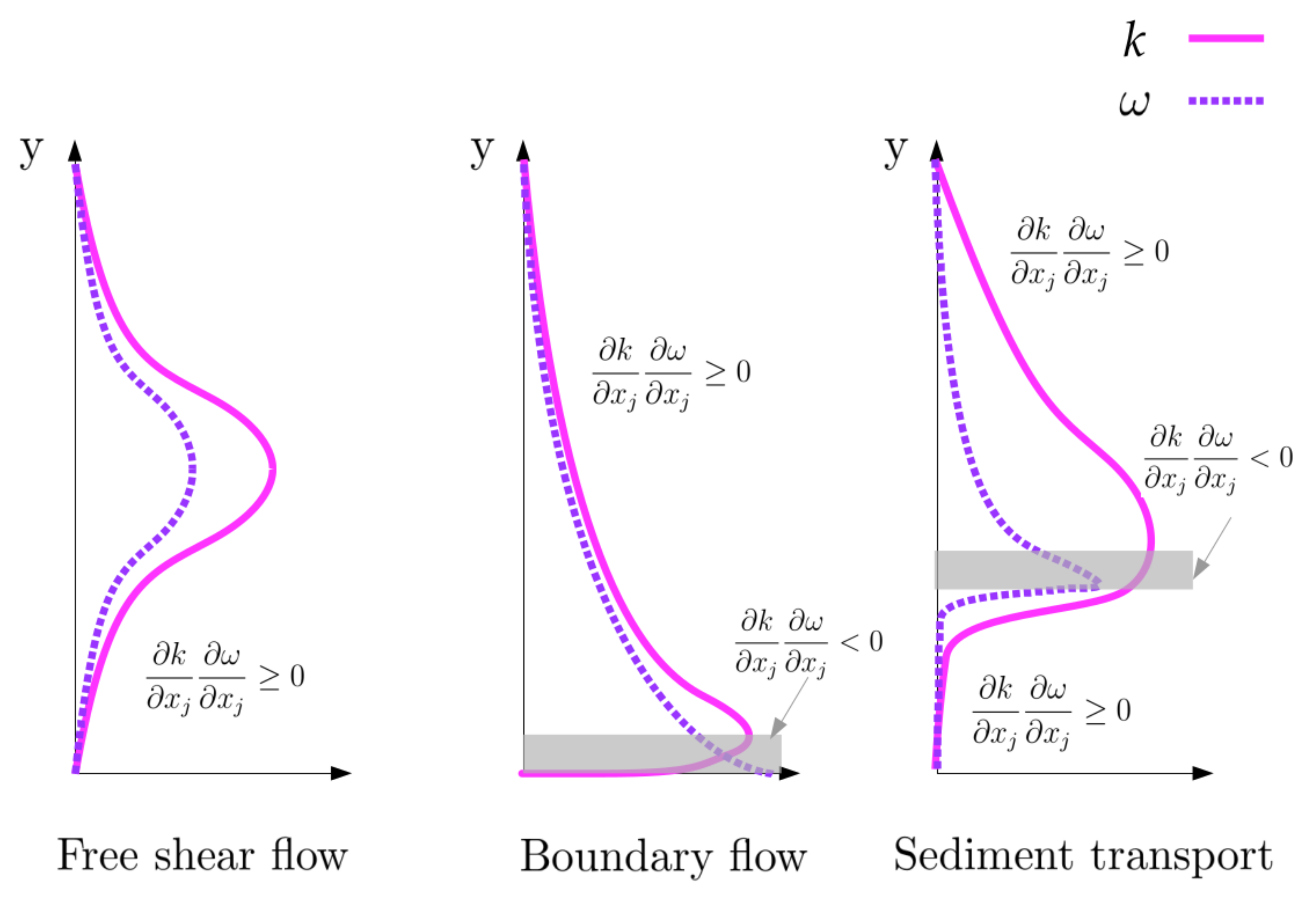
2.3.3. Modified Model
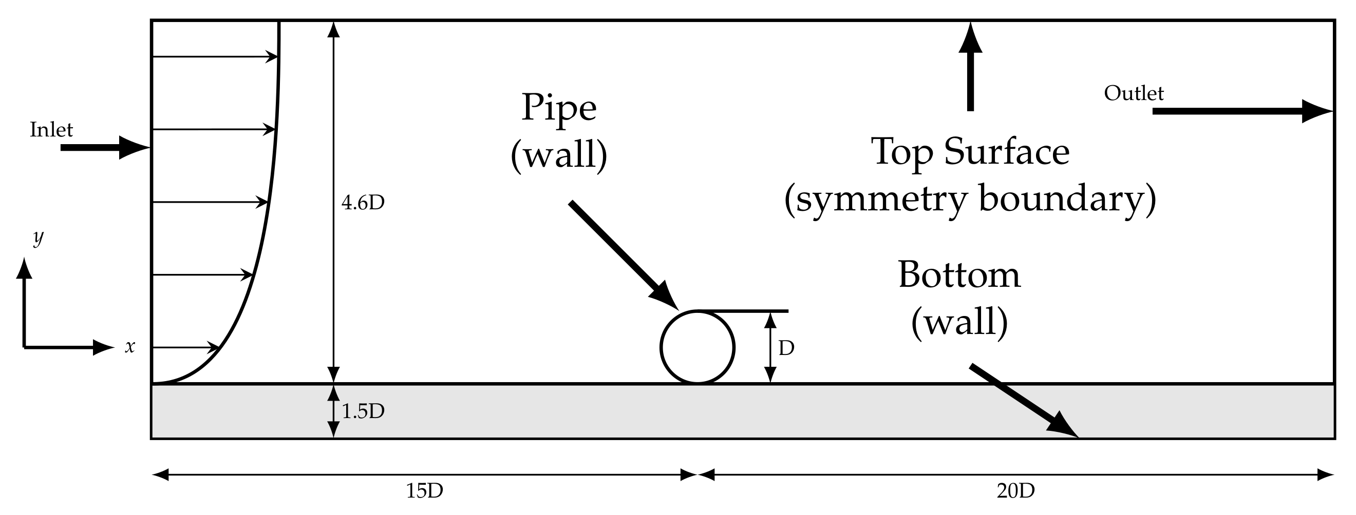
2.4. Numerical Setup
2.4.1. General Setup
2.4.2. Simulations with the Turbulence Model
2.4.3. Simulations with the 2006 and the Modified Turbulence Models
2.5. Brier Skill Score
3. Results
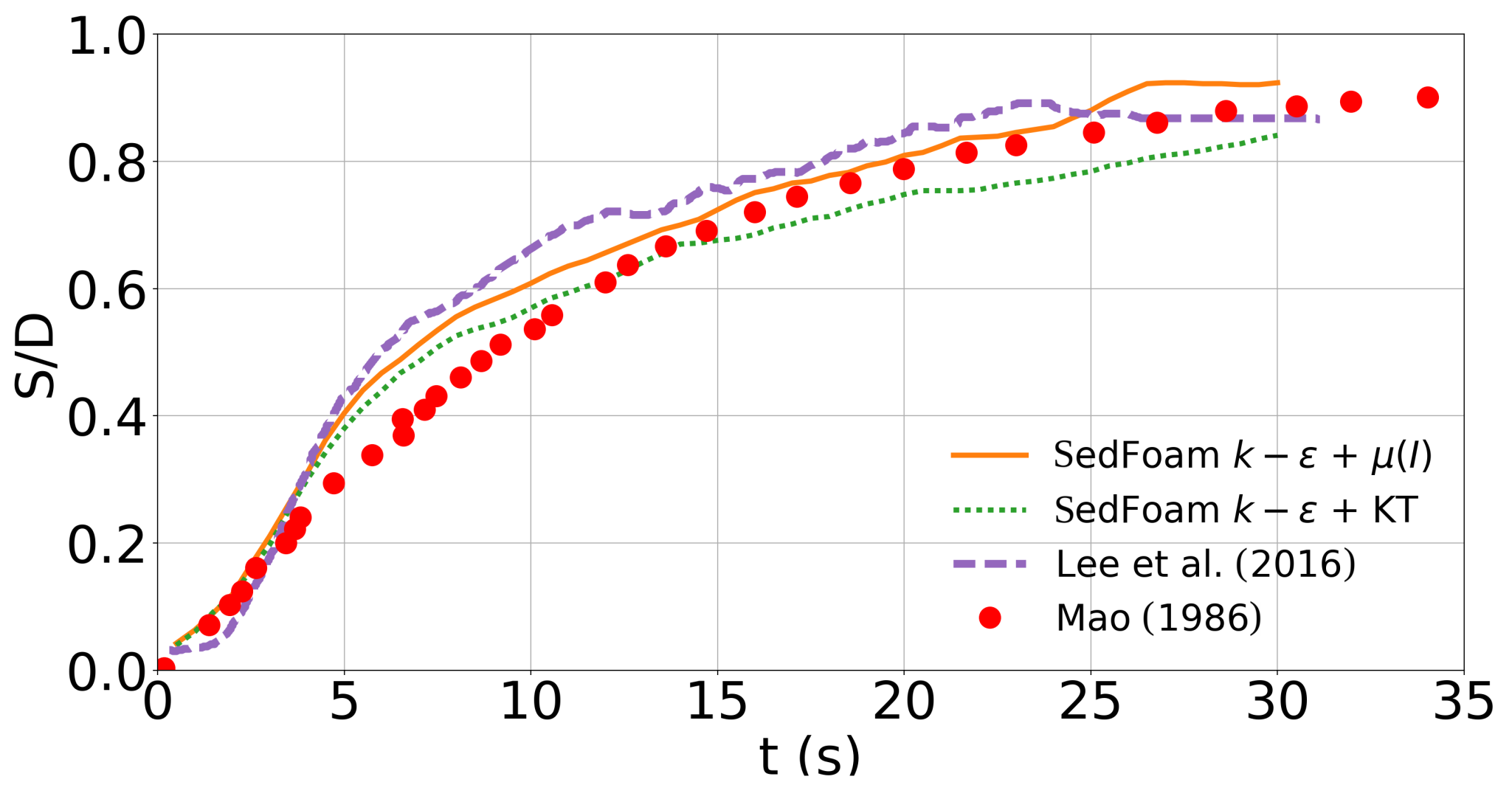
3.1. Solid Phase Stress Model Sensitivity
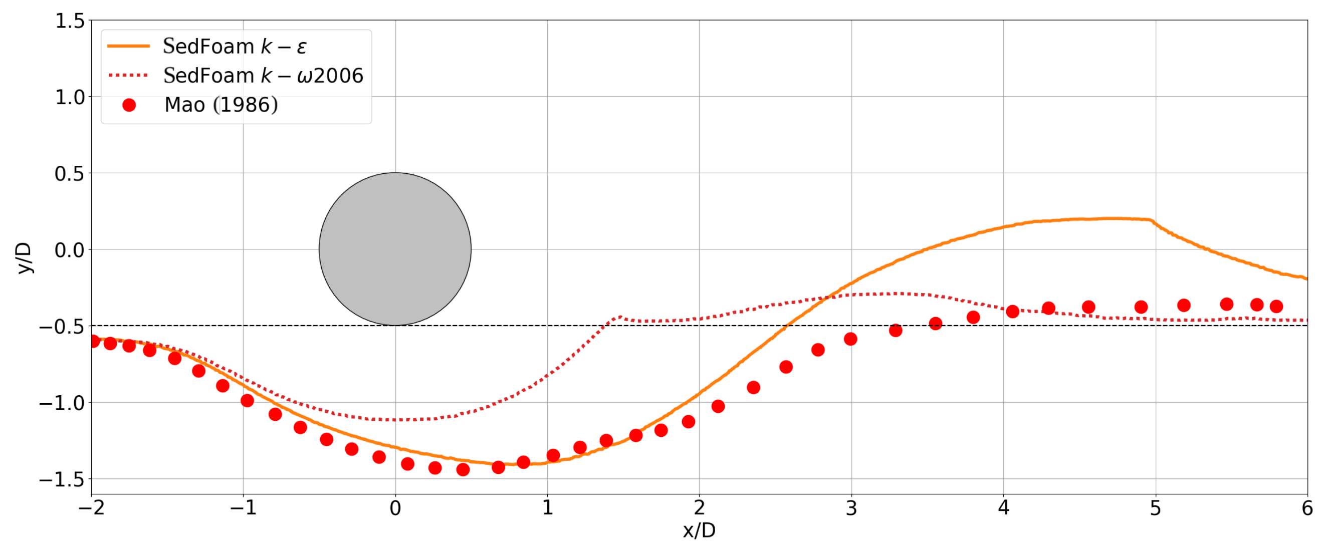
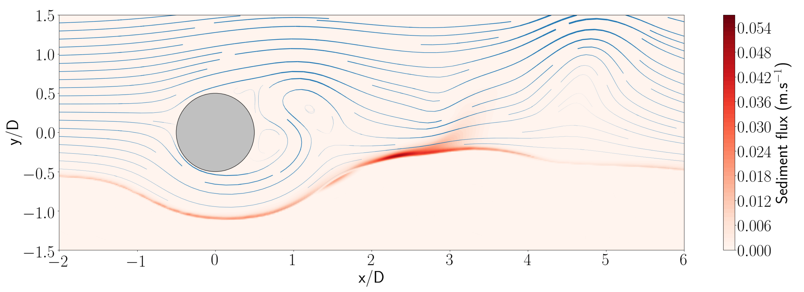
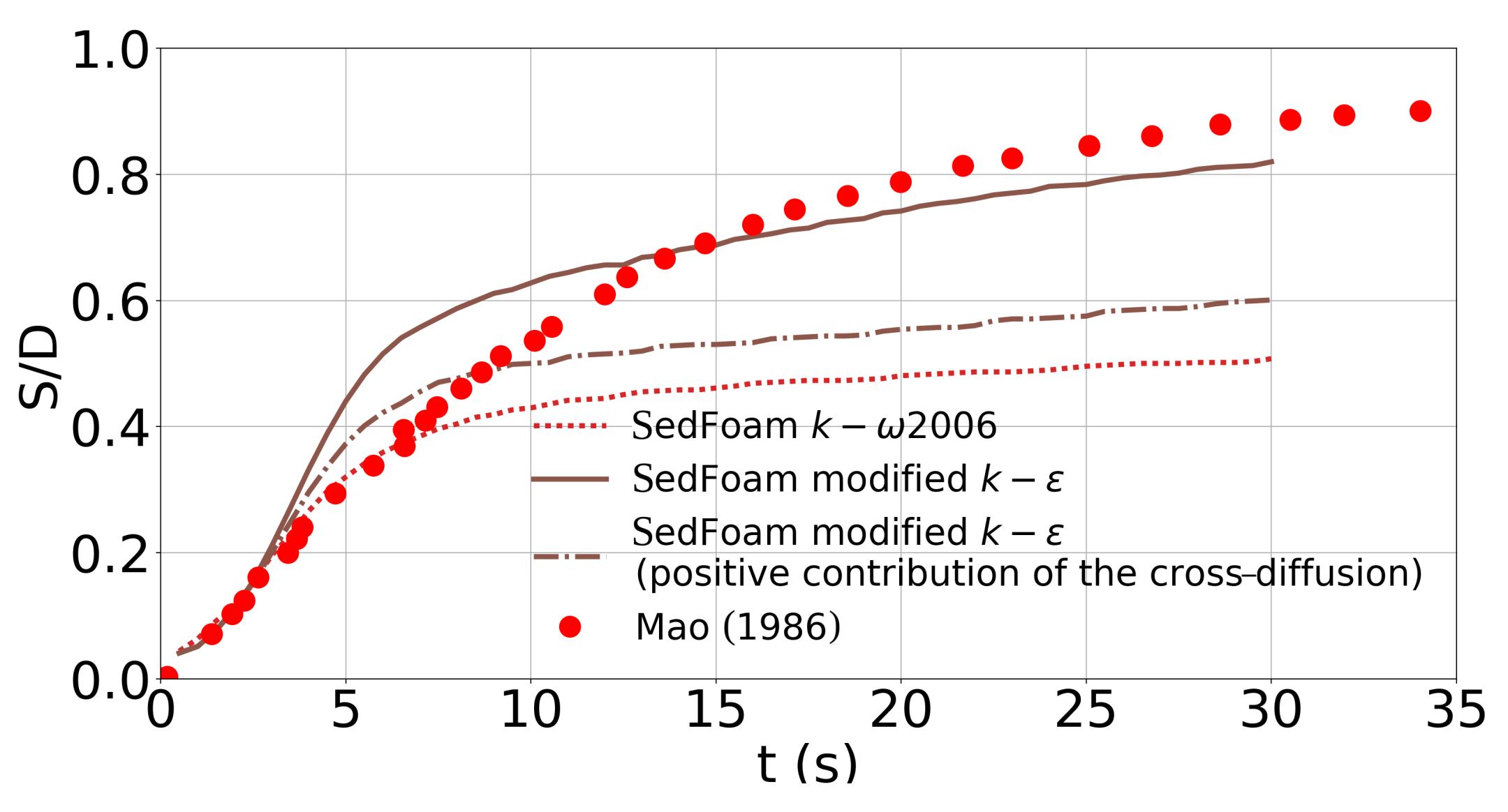
3.2. Turbulence Model Sensitivity
4. Discussion
5. Conclusions
Author Contributions
Funding
Acknowledgments
Conflicts of Interest
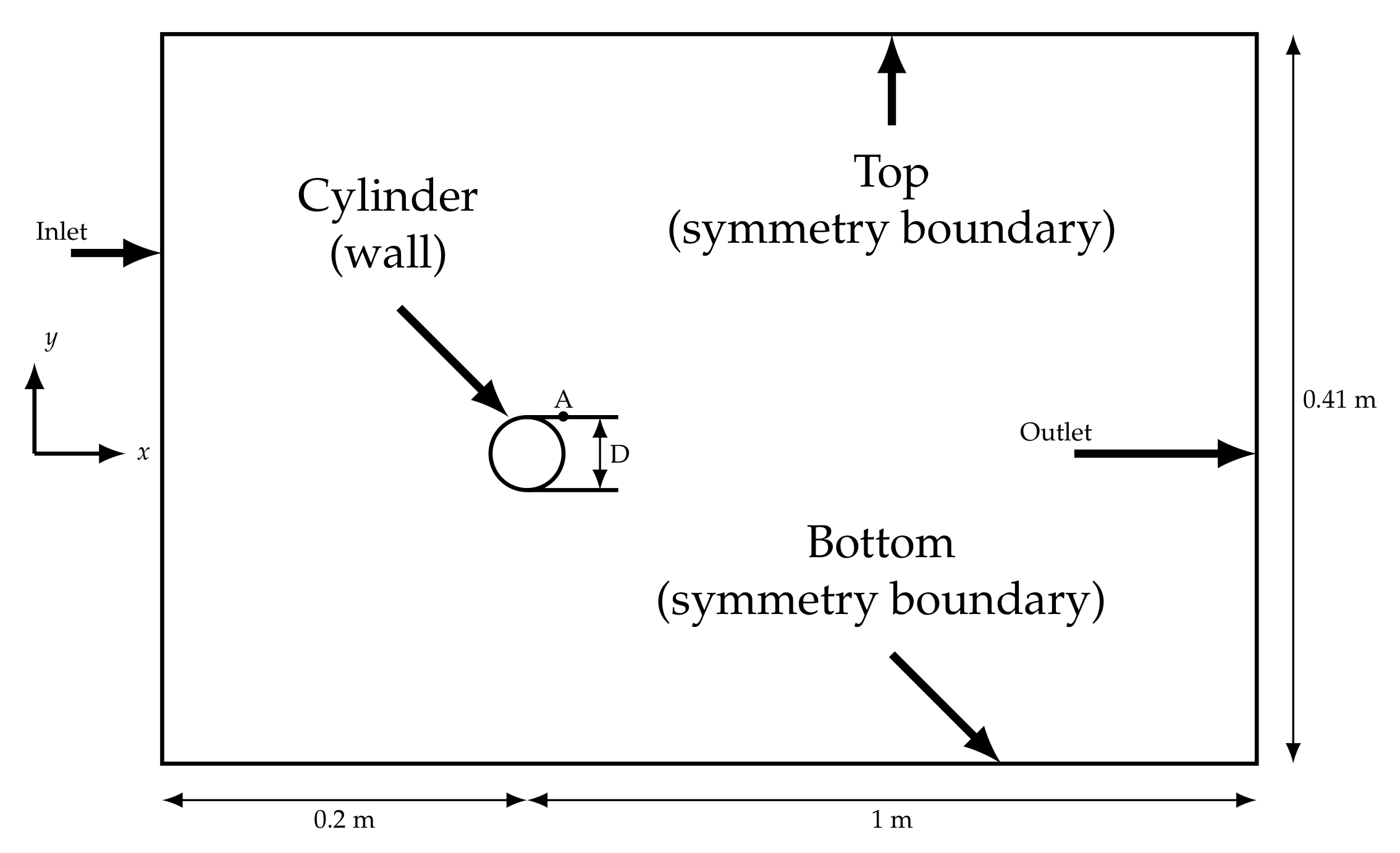
Appendix A. Hydrodynamic Simulations
Appendix A.1. Numerical Setup


| Turbulence Kinetic Energy | Dissipation | |
|---|---|---|
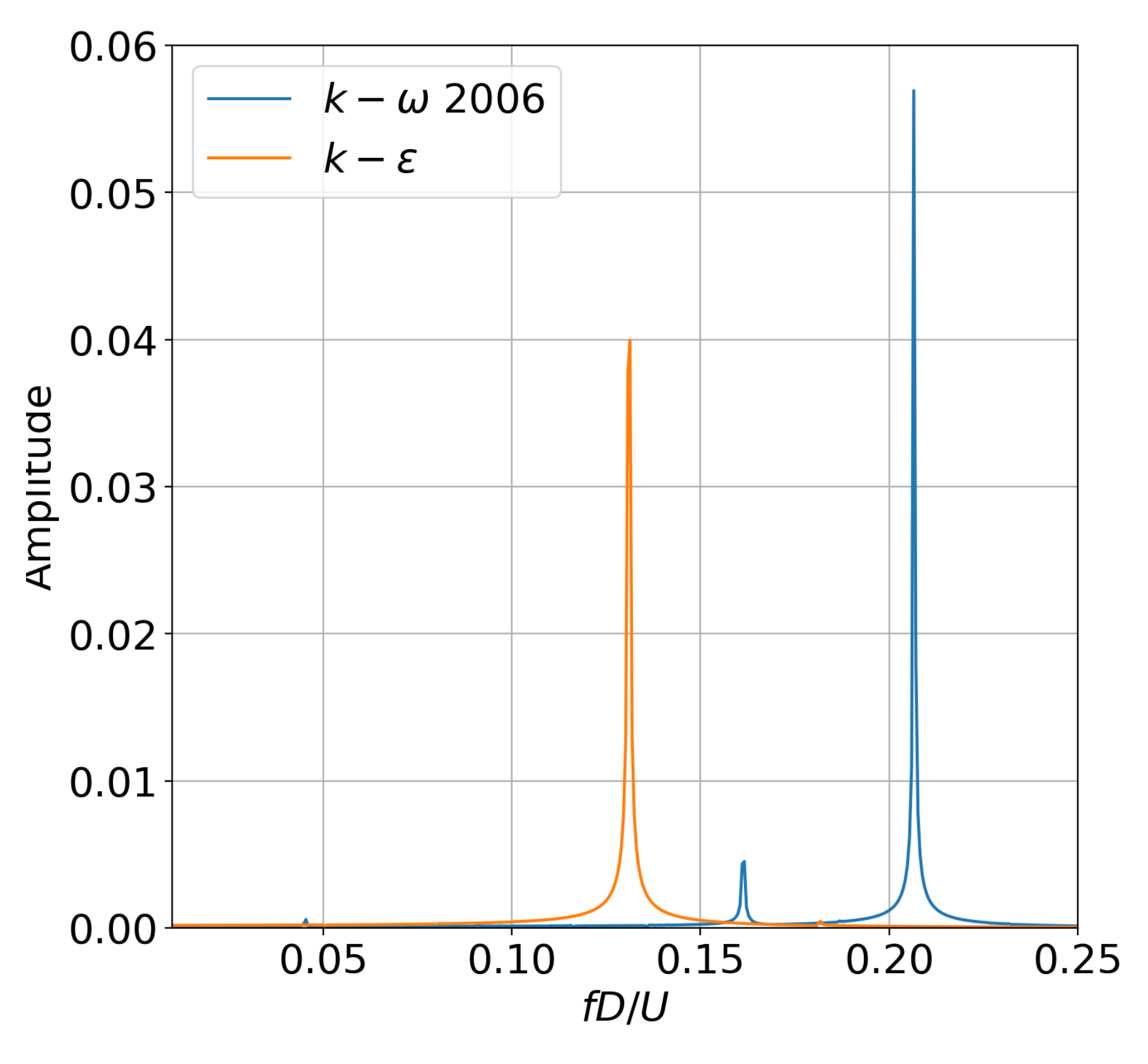
Appendix A.2. Results

References
- Sumer, B.M.; Fredsoe, J. The Mechanics of Scour in the Marine Environment; World Scientific Publishing Company: Singapore, 2002; Volume 17. [Google Scholar]
- Mao, Y. The Interaction Between a Pipeline and an Erodible Bed; Institute of Hydrodynamics and Hydraulic Engineering København: Series Paper; Institute of Hydrodynamics and Hydraulic Engineering; Technical University of Denmark: Lyngby, Denmark, 1986. [Google Scholar]
- Chiew, Y. Prediction of Maximum Scour Depth at Submarine Pipelines. J. Hydraul. Eng. 1991, 117, 452–466. [Google Scholar] [CrossRef]
- Li, F.; Cheng, L. Numerical Model for Local Scour under Offshore Pipelines. J. Hydraul. Eng. 1999, 125, 400–406. [Google Scholar] [CrossRef]
- Leeuwenstein, W.; Wind, H.G. The Computation of Bed Shear in a Numerical Model. In Proceedings of the 19th International Conference on Coastal Engineering, Houston, TX, USA, 3–7 September 1985. [Google Scholar]
- Liang, D.; Cheng, L.; Li, F. Numerical modeling of flow and scour below a pipeline in currents: Part II. Scour simulation. Coast. Eng. 2005, 52, 43–62. [Google Scholar] [CrossRef]
- Jenkins, J.T.; Hanes, D.M. Collisional sheet flows of sediment driven by a turbulent fluid. J. Fluid Mech. 1998, 370, 29–52. [Google Scholar] [CrossRef]
- Revil-Baudard, T.; Chauchat, J. A two-phase model for sheet flow regime based on dense granular flow rheology. J. Geophys. Res. Ocean. 2013, 118, 619–634. [Google Scholar] [CrossRef]
- Hsu, T.J.; Liu, P.L.F. Toward modeling turbulent suspension of sand in the nearshore. J. Geophys. Res. Ocean. 2004, 109. [Google Scholar] [CrossRef]
- Zhao, Z.; Fernando, H.J.S. Numerical simulation of scour around pipelines using an Euler-Euler coupled two-phase model. Environ. Fluid Mech. 2007, 7, 121–142. [Google Scholar] [CrossRef]
- Yeganeh-Bakhtiary, A.; Kazeminezhad, M.H.; Etemad-Shahidi, A.; Baas, J.H.; Cheng, L. Euler-Euler two-phase flow simulation of tunnel erosion beneath marine pipelines. Appl. Ocean Res. 2011, 33, 137–146. [Google Scholar] [CrossRef]
- Lee, C.H.; Low, Y.M.; Chiew, Y.M. Multi-dimensional rheology-based two-phase model for sediment transport and applications to sheet flow and pipeline scour. Phys. Fluids 2016, 28, 053305. [Google Scholar] [CrossRef]
- MiDi, G.D.R. On dense granular flows. Eur. Phys. J. E 2004, 14, 341–365. [Google Scholar] [CrossRef]
- Wilcox, D.C. Turbulence Modeling for CFD; DCW Industries: La Canada, CA, USA, 2006. [Google Scholar]
- Nagel, T. Three-Dimensional Scour Simulations with a Two-Phase Flow Model. 2019; under review. [Google Scholar]
- Cheng, Z.; Hsu, T.J.; Calantoni, J. SedFoam: A multi-dimensional Eulerian two-phase model for sediment transport and its application to momentary bed failure. Coast. Eng. 2017, 119, 32–50. [Google Scholar] [CrossRef]
- Chauchat, J.; Cheng, Z.; Nagel, T.; Bonamy, C.; Hsu, T.J. SedFoam-2.0: A 3D two-phase flow numerical model for sediment transport. Geosci. Model Dev. Discuss. 2017, 10, 4367–4392. [Google Scholar] [CrossRef]
- Boyer, F.; Guazzelli, E.; Pouliquen, O. Unifying Suspension and Granular Rheology. Phys. Rev. Lett. 2011, 107, 188301. [Google Scholar] [CrossRef]
- Richardson, J.F.; Zaki, W. Sedimentation and Fluidization: Part I. Chem. Eng. Res. Des. 1954, 32, 35–53. [Google Scholar]
- Schiller, L.; Naumann, A.Z. Über die grundlegenden Berechnungen bei der Schwerkraftaufbereitung. Ver. Deut. Ing. 1933, 77, 318–320. [Google Scholar]
- Chauchat, J. A comprehensive two-phase flow model for unidirectional sheet-flows. J. Hydraul. Res. 2017, 2017, 1289260. [Google Scholar] [CrossRef]
- Maurin, R.; Chauchat, J.; Frey, P. Dense granular flow rheology in turbulent bedload transport. J. Fluid Mech. 2016, 804, 490–512. [Google Scholar] [CrossRef]
- Jop, P.; Forterre, Y.; Pouliquen, O. A constitutive law for dense granular flows. Nature 2006, 441, 727–730. [Google Scholar] [CrossRef]
- Chauchat, J.; Marc, M. A three-dimensional numerical model for incompressible two-phase flow of a granular bed submitted to a laminar shearing flow. Comput. Methods Appl. Mech. Eng. 2009, 199, 439–449. [Google Scholar] [CrossRef]
- Ding, J.; Gidaspow, D. A bubbling fluidization model using kinetic theory of granular flow. AIChE J. 1990, 36, 523–538. [Google Scholar] [CrossRef]
- Carnahan, N.F.; Starling, K.E. Equation of State for Nonattracting Rigid Spheres. J. Chem. Phys. 1969, 51, 635–636. [Google Scholar] [CrossRef]
- Van Rijn, L. Sediment Transport, Part II: Suspended Load Transport. J. Hydraul. Eng. 1984, 110, 1613–1641. [Google Scholar] [CrossRef]
- Ferziger, J.H.; Peric, M. Computational Methods for Fluid Dynamics; Springer Science & Business Media: Berlin/Heidelberg, Germany, 2002. [Google Scholar]
- Sutherland, J.; Hall, L.; Chesher, T. Evaluation of the Coastal Area Model PISCES at Teignmouth (UK); HR Wallingford Report TR125; 2001. [Google Scholar] [CrossRef]
- Brady, A.; Sutherland, J. COSMOS Modelling of COAST3D Egmond Main Experiment; HR Wallingford Report TR115; 2001. [Google Scholar] [CrossRef]
- Van Rijn, L.; Ruessink, B.; Mulder, J. Coast3D-Egmond: The Behaviour of a Straight Sandy Coast on the Time Scale of Storms and Seasons; Aqua Publications: Locust Valley, NY, USA, 2002. [Google Scholar]
- Sumer, B.; Fredsoe, J. Hydrodynamics Around Cylindrical Structures; World Scientific: Singapore, 2006; Volume 12. [Google Scholar]


| 1.0 | 0.77 | 1.44 | 1.92 | 1.2 | 1.0 | 0.09 |
| C | |||||||
|---|---|---|---|---|---|---|---|
| 0.6 | 0.5 | 0.52 | 0.0708 | 0.35 | 1.0 | 0.09 | 0.875 |
| 1.0 | 0.856 | 0.44 | 0.0828 | 0.35 | 1.0 | 1.712 or Equation (32) |
© 2019 by the authors. Licensee MDPI, Basel, Switzerland. This article is an open access article distributed under the terms and conditions of the Creative Commons Attribution (CC BY) license (http://creativecommons.org/licenses/by/4.0/).
Share and Cite
Mathieu, A.; Chauchat, J.; Bonamy, C.; Nagel, T. Two-Phase Flow Simulation of Tunnel and Lee-Wake Erosion of Scour below a Submarine Pipeline. Water 2019, 11, 1727. https://doi.org/10.3390/w11081727
Mathieu A, Chauchat J, Bonamy C, Nagel T. Two-Phase Flow Simulation of Tunnel and Lee-Wake Erosion of Scour below a Submarine Pipeline. Water. 2019; 11(8):1727. https://doi.org/10.3390/w11081727
Chicago/Turabian StyleMathieu, Antoine, Julien Chauchat, Cyrille Bonamy, and Tim Nagel. 2019. "Two-Phase Flow Simulation of Tunnel and Lee-Wake Erosion of Scour below a Submarine Pipeline" Water 11, no. 8: 1727. https://doi.org/10.3390/w11081727
APA StyleMathieu, A., Chauchat, J., Bonamy, C., & Nagel, T. (2019). Two-Phase Flow Simulation of Tunnel and Lee-Wake Erosion of Scour below a Submarine Pipeline. Water, 11(8), 1727. https://doi.org/10.3390/w11081727