Dynamics of Sediment Transport and Erosion-Deposition Patterns in the Locality of a Detached Low-Crested Breakwater on a Cohesive Coast


Abstract
1. Introduction
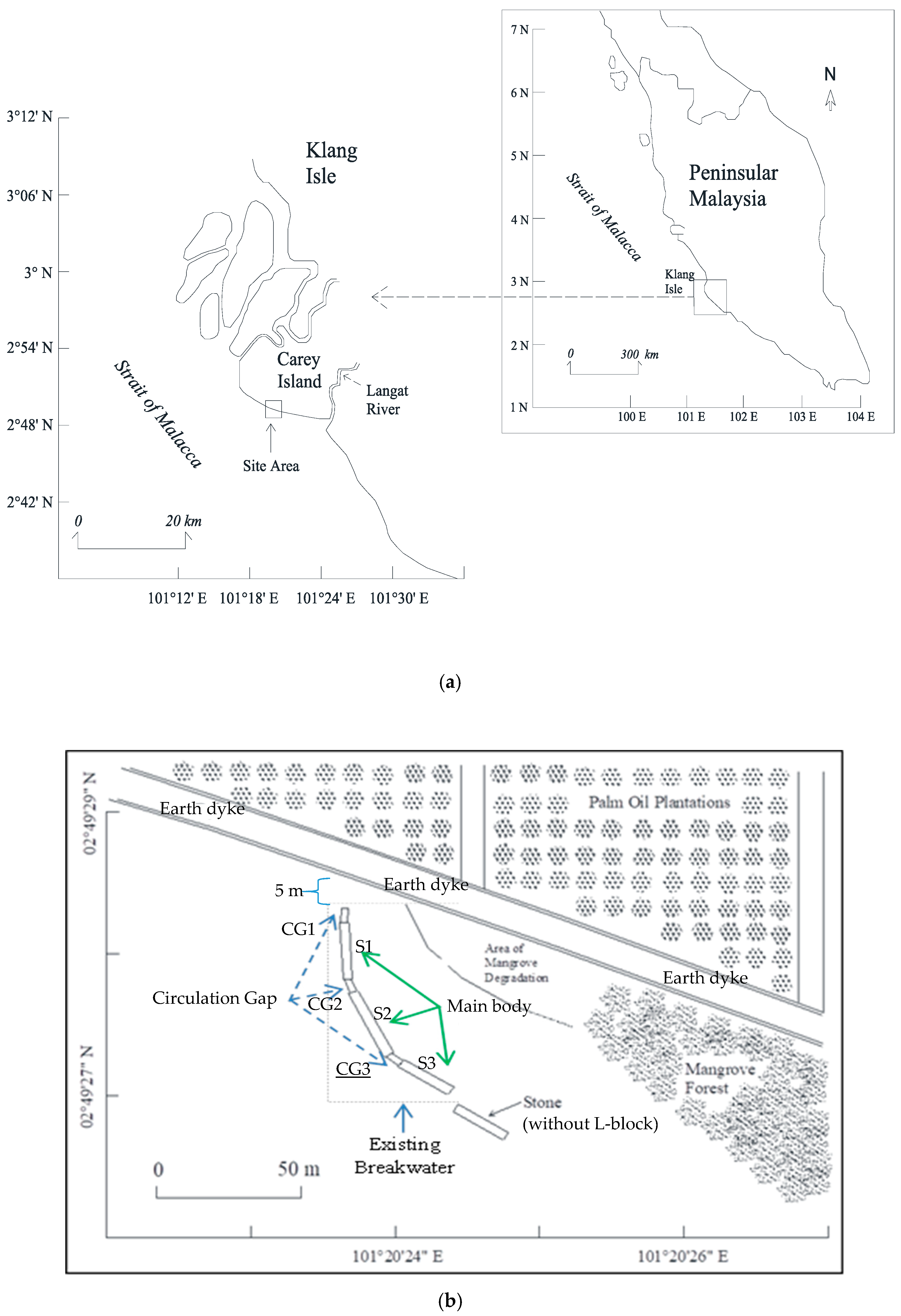
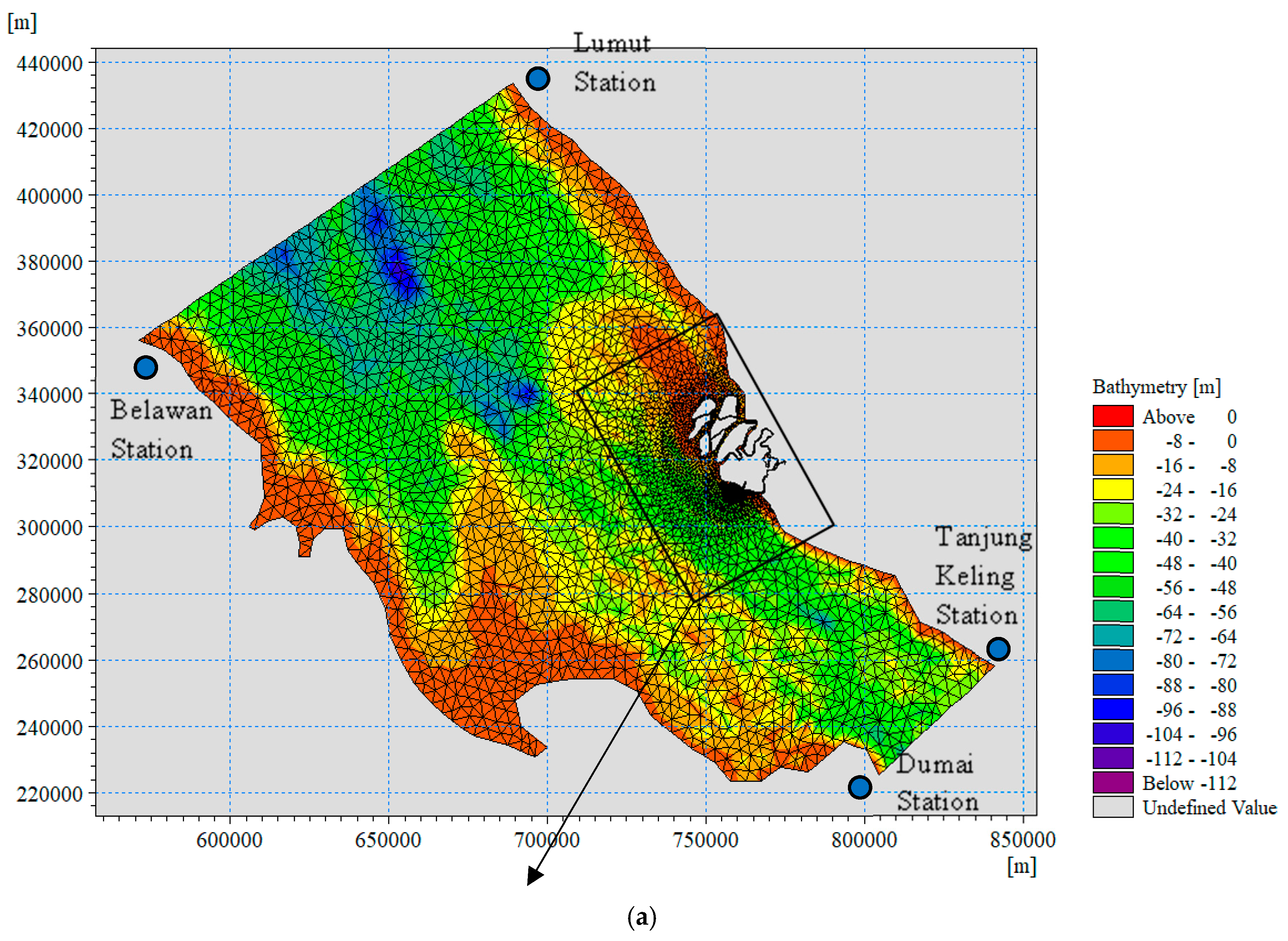
2. Study Area
3. Methods
3.1. Data Collection
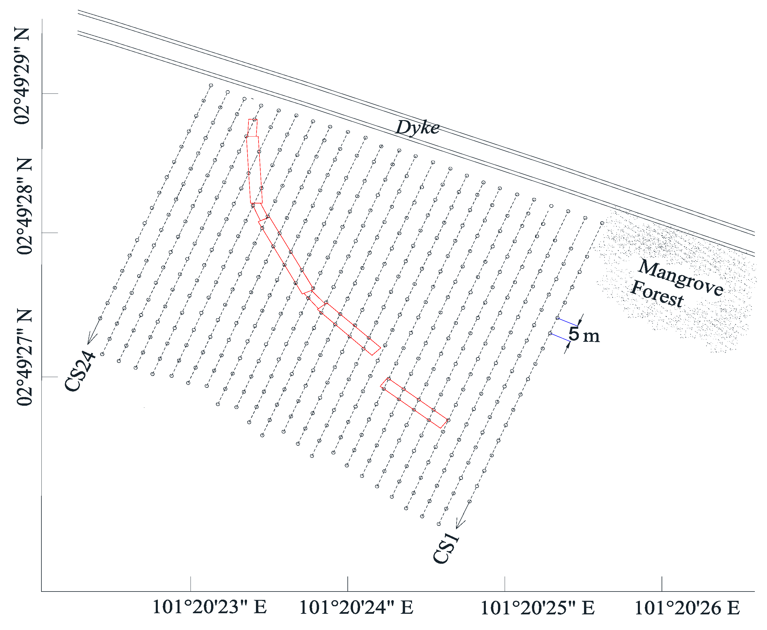
3.2. Monitoring of Sea-Bed Elevation
3.3. Numerical Modelling
3.3.1. Model Setup
3.3.2. Model Input
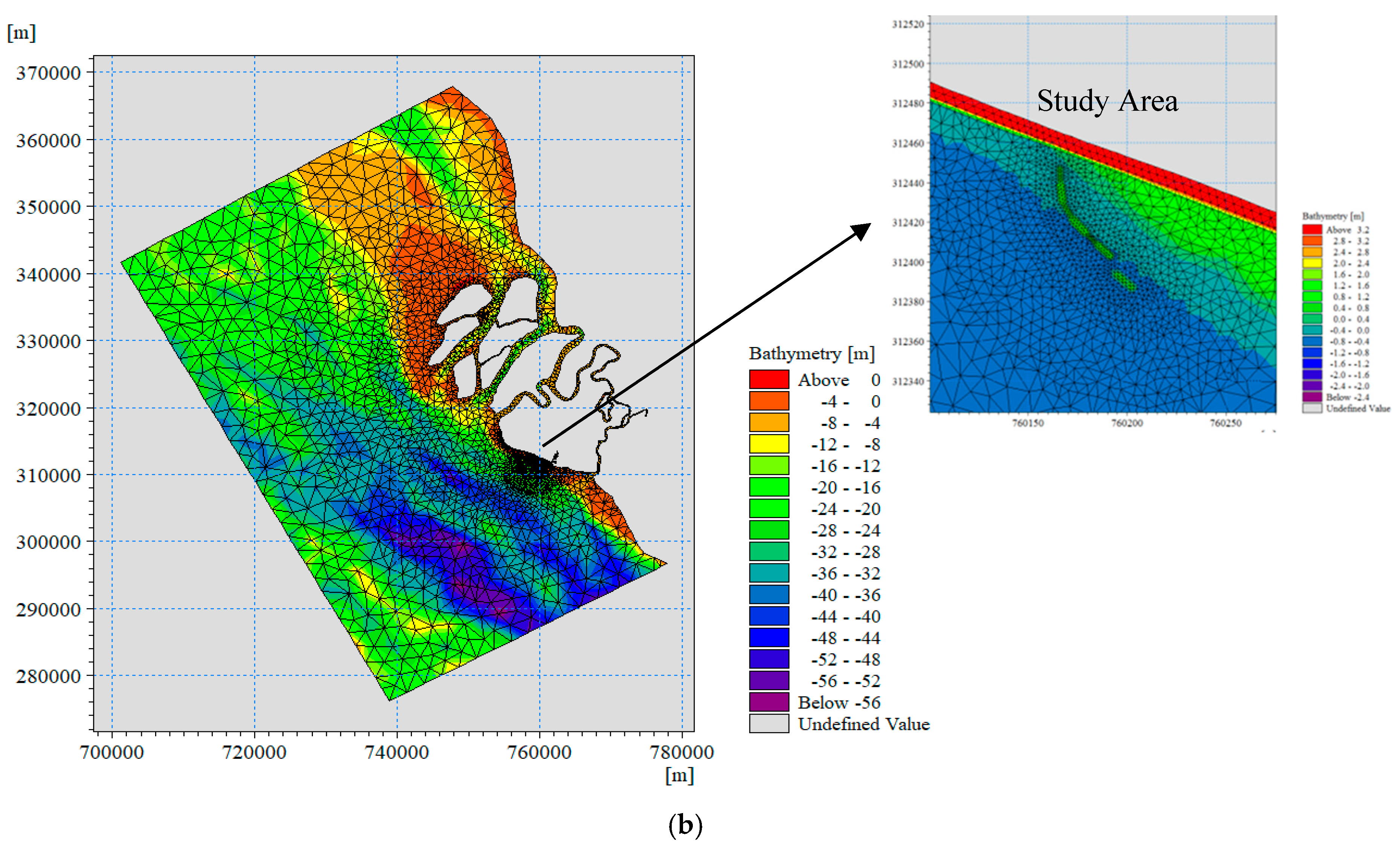
3.3.3. Computational Domain
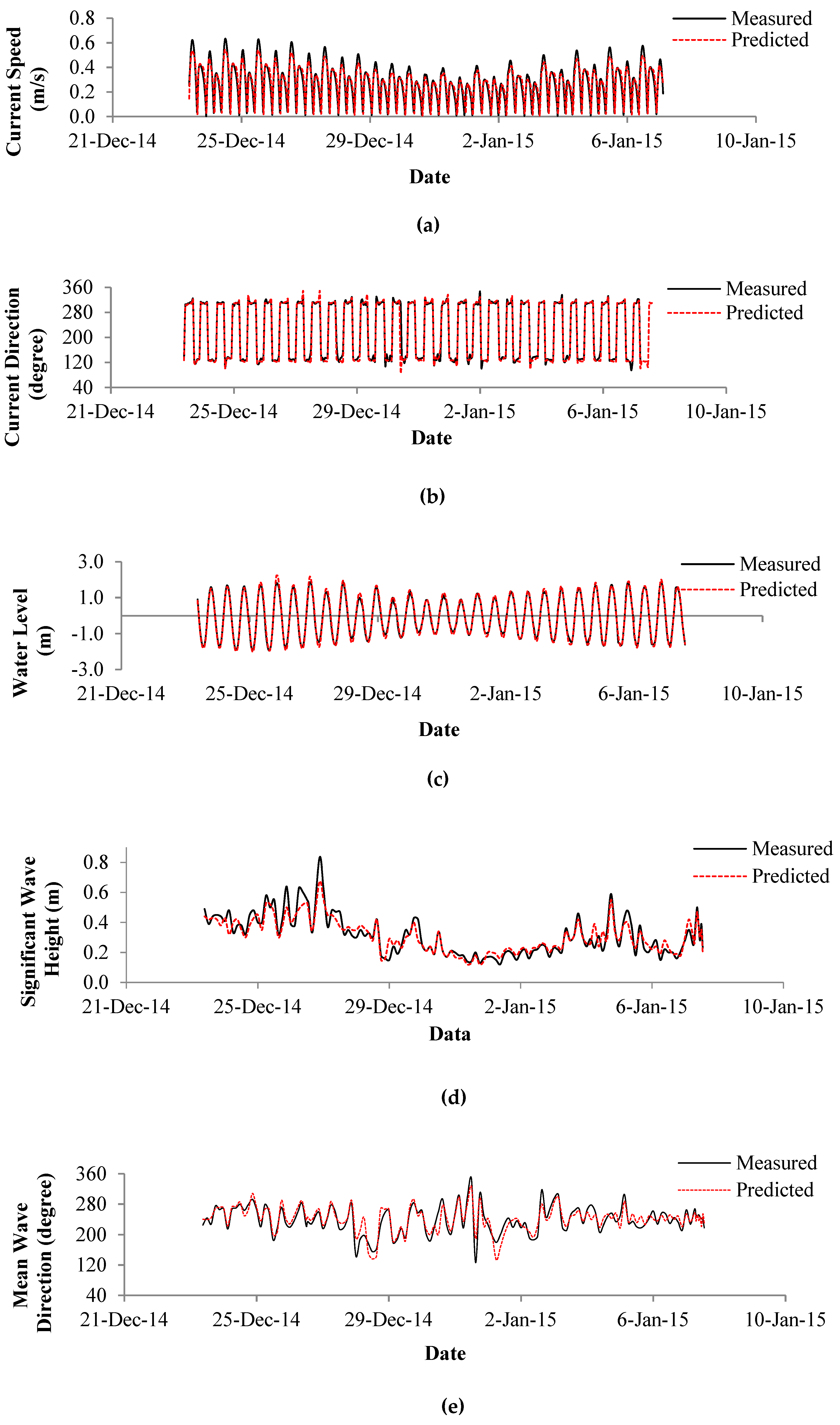
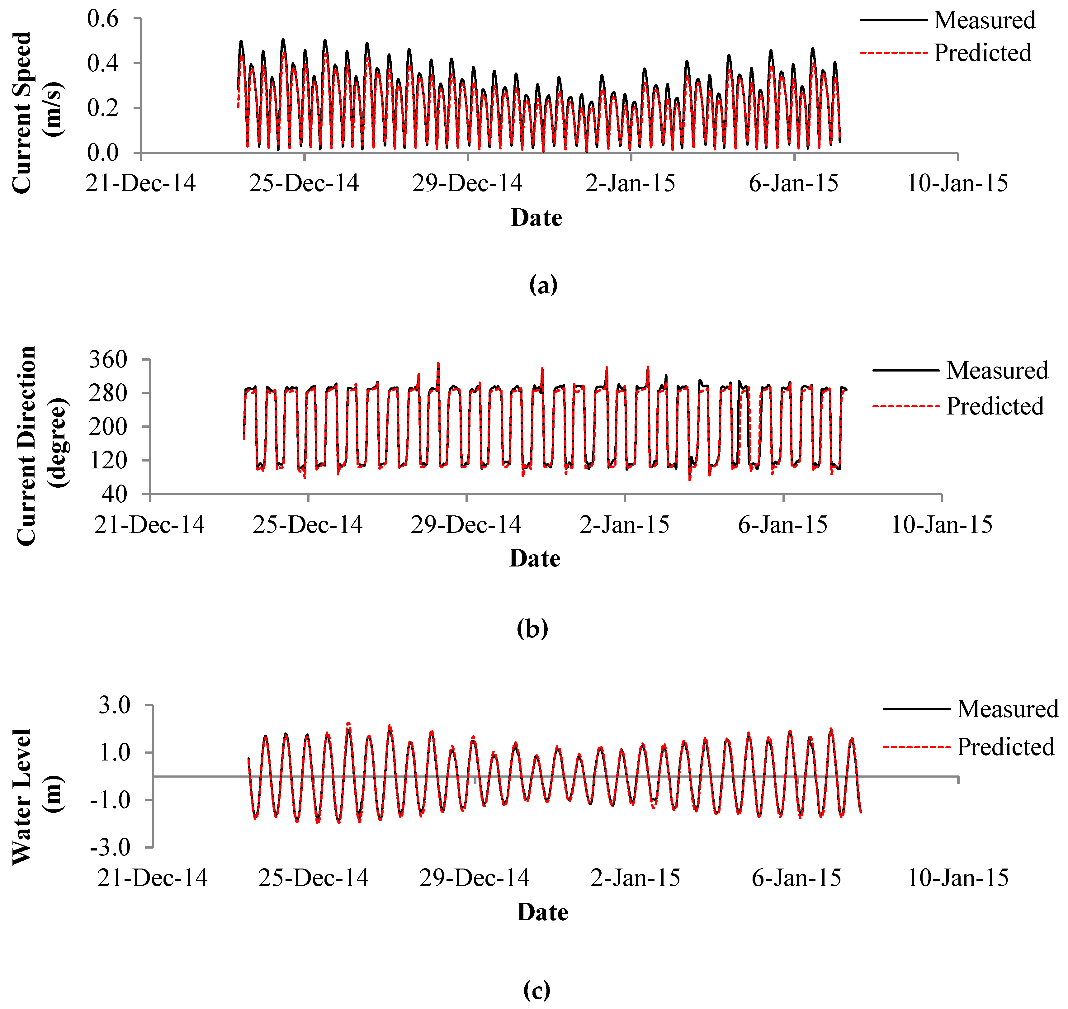
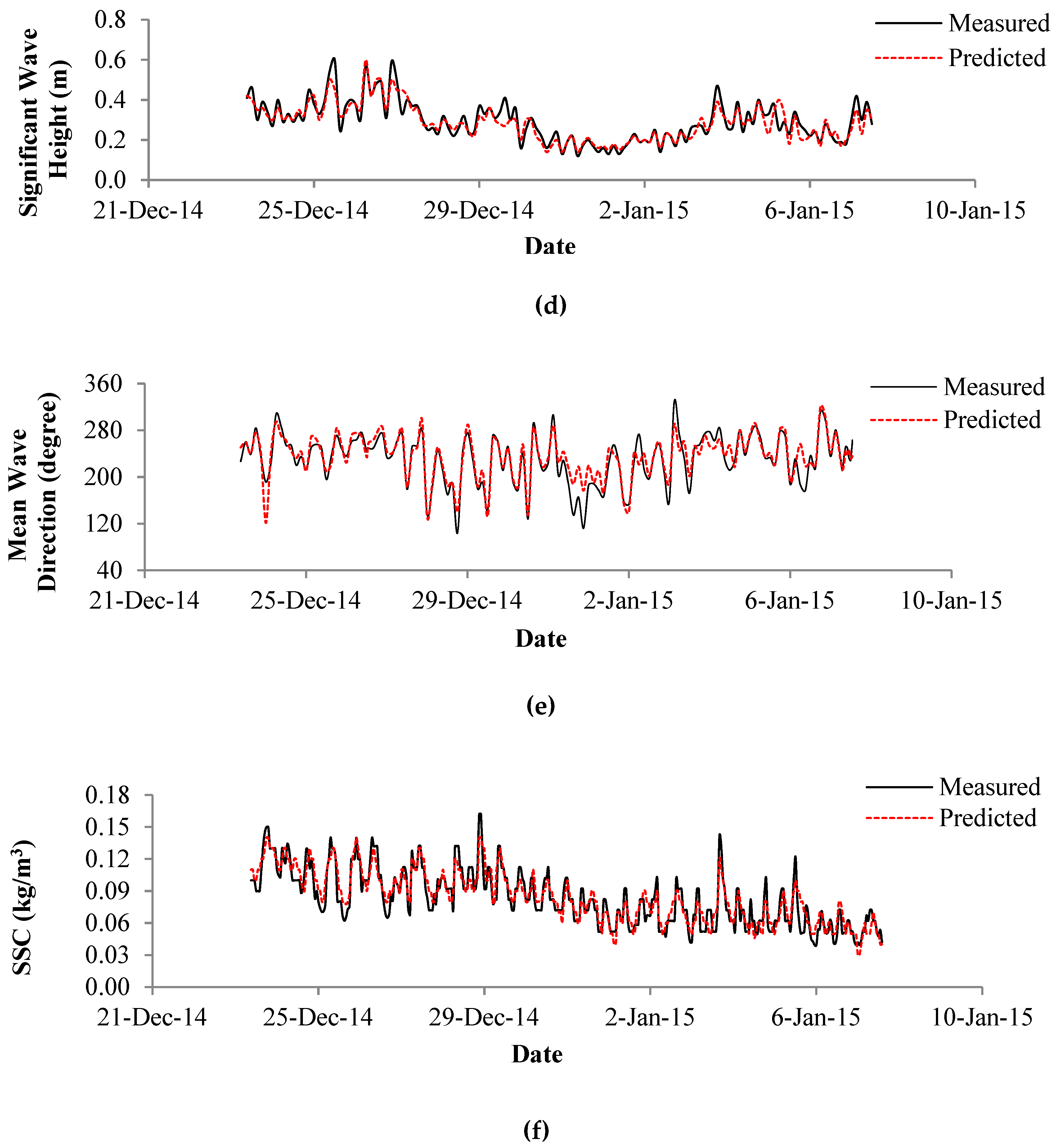
3.3.4. Model Calibration and Validation
4. Results and Discussion
4.1. Sediment and Water Samples Analyses
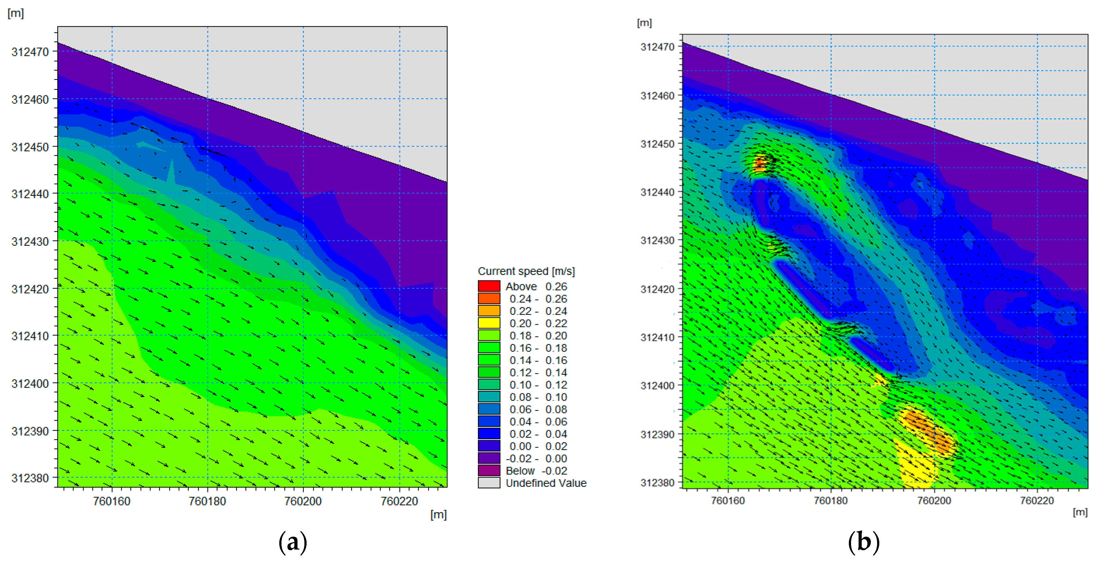
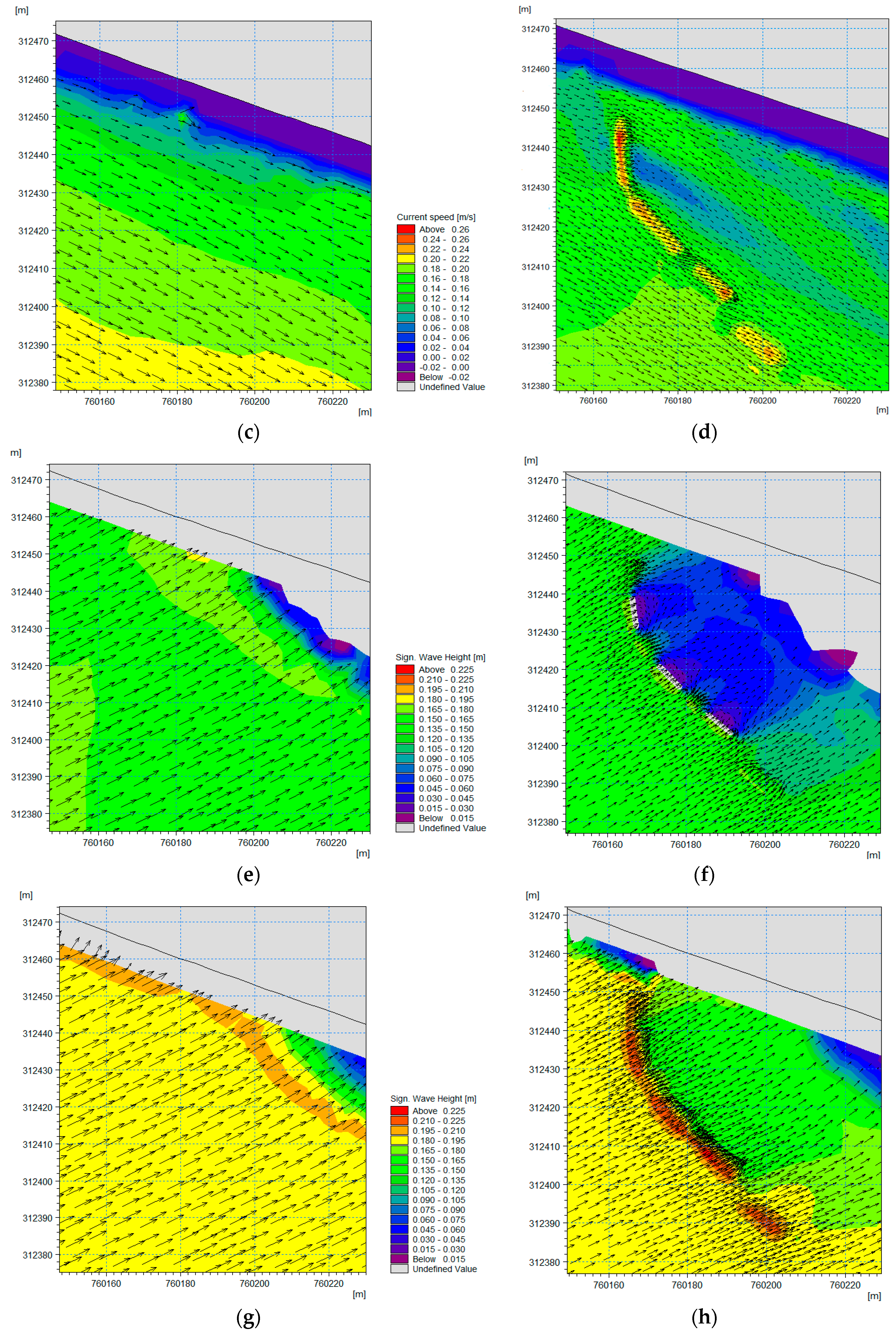
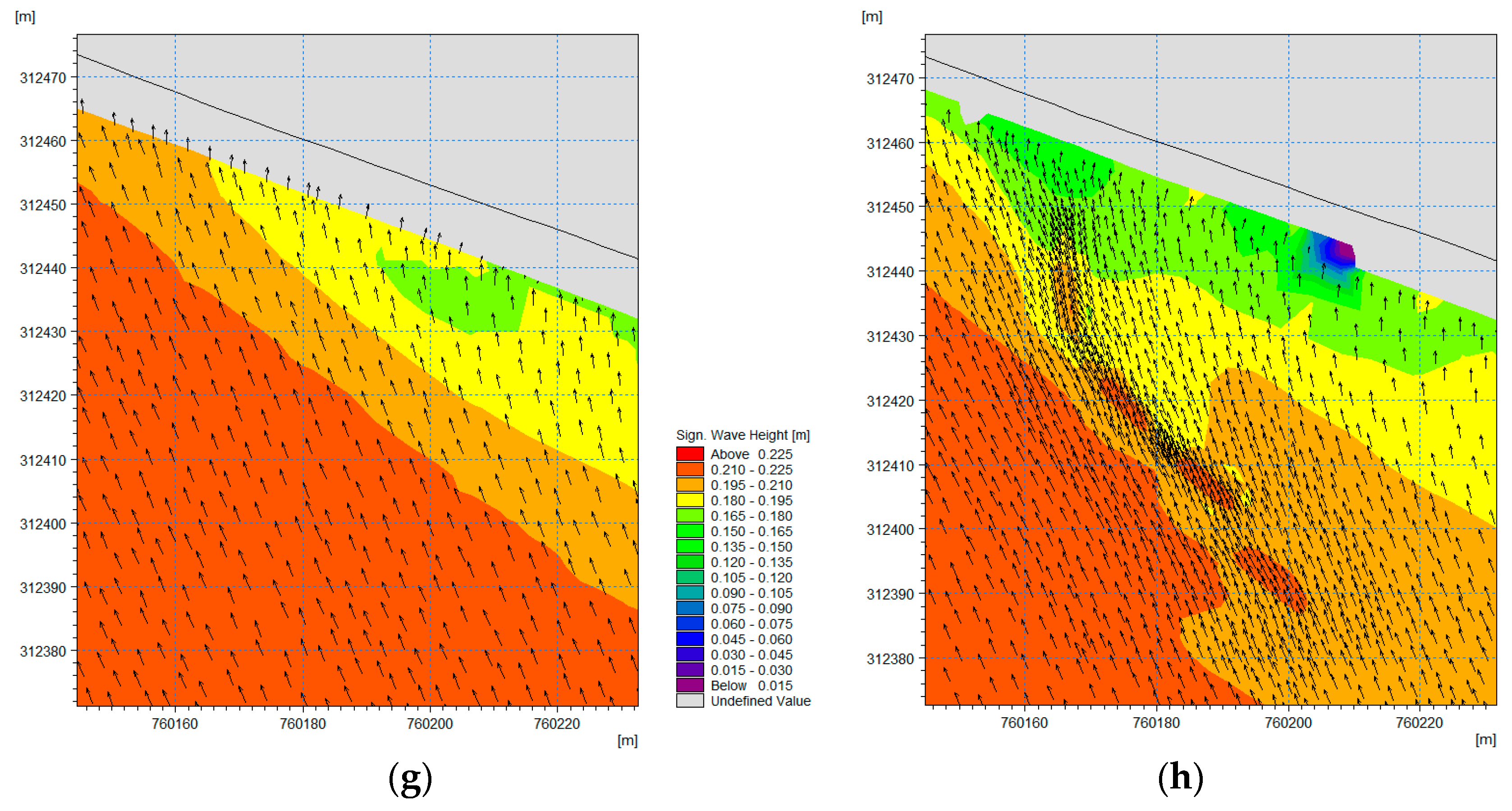
4.2. Hydrodynamic Changes in the Locality of the Breakwater Structure
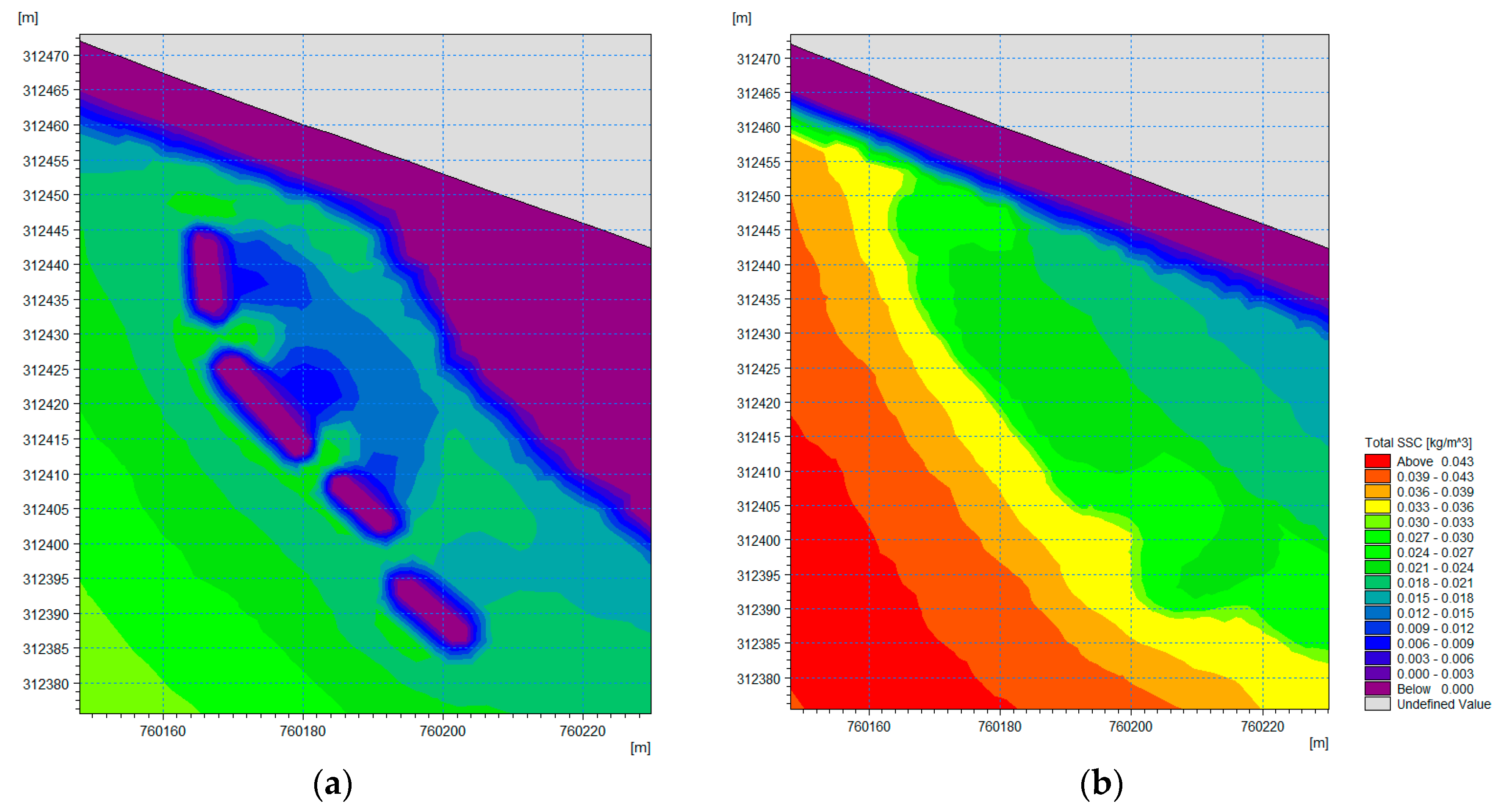
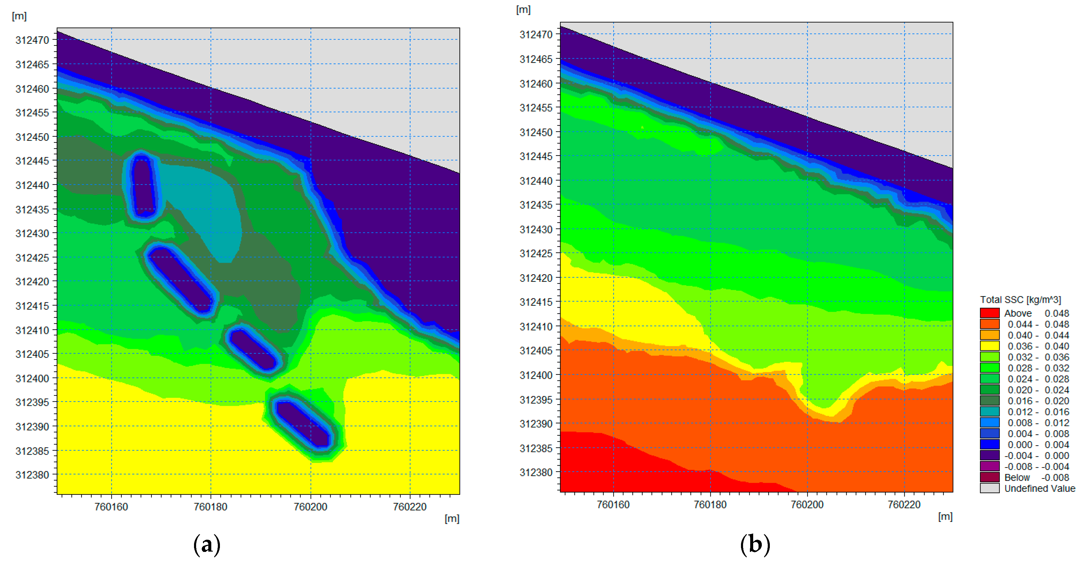
4.3. Suspended Sediment Transport in the Breakwater’s Surroundings
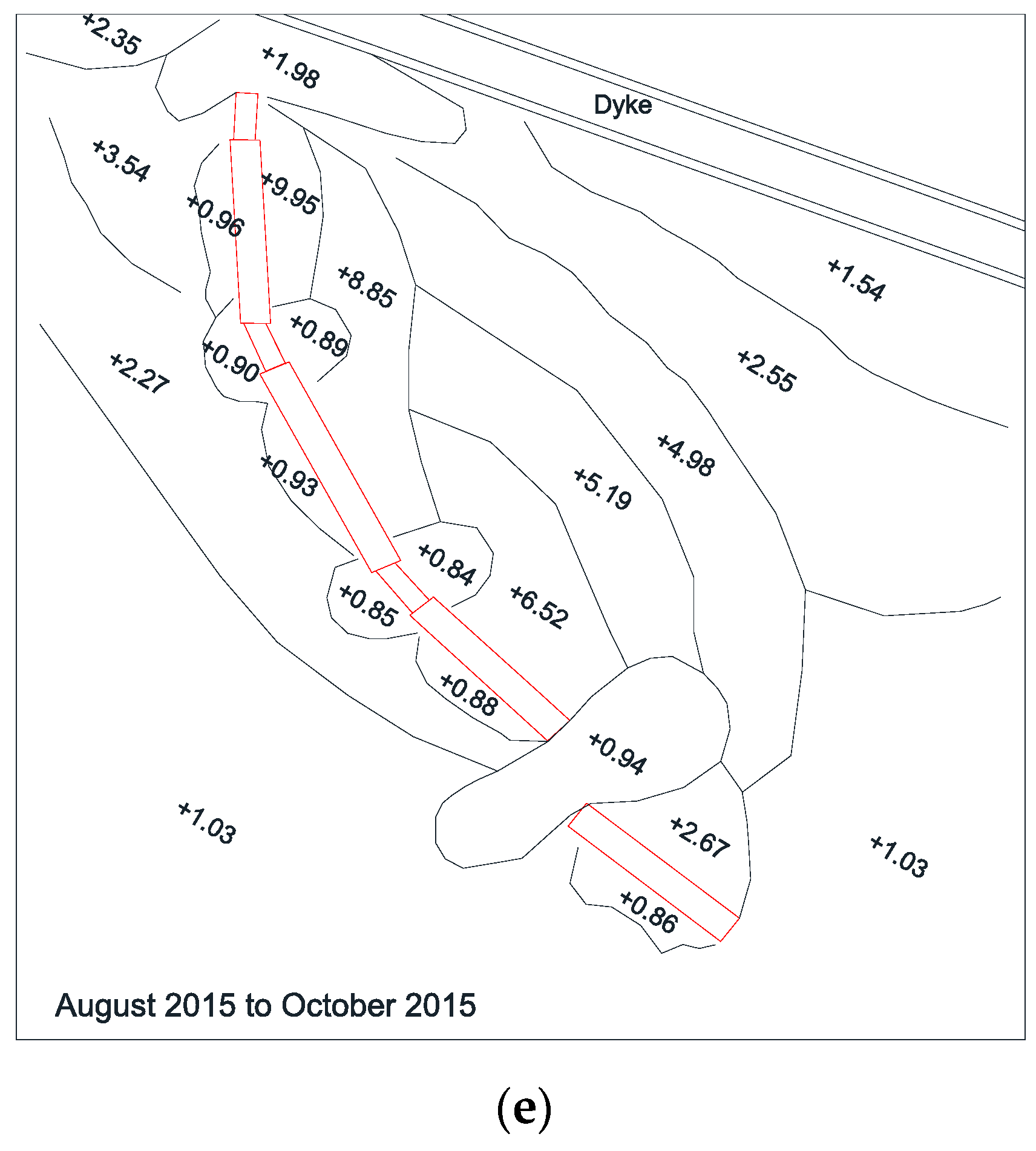
4.4. Variation of Sea-Bed Levels and Erosion-Deposition Pattern in the Locality of the Low-Crested Breakwater
4.5. Discussion
4.5.1. Sediment Transport and Erosion-Deposition Pattern during the Northeast Season
4.5.2. Sediment Transport and Erosion-Deposition Pattern during the Southwest Season
5. Conclusions
Author Contributions
Funding
Acknowledgments
Conflicts of Interest
References
- Hashim, R.; Kamali, B.; Tamin, N.M.; Zakaria, R. An integrated approach to coastal rehabilitation: Mangrove restoration in Sungai Haji Dorani, Malaysia. Estuar. Coast. Shelf Sci. 2010, 86, 118–124. [Google Scholar] [CrossRef]
- Hashim, R.; Fitri, A.; Motamedi, S.; Hashim, A.M. Modeling of Coastal Hydrodynamic Associated with Coastal Structures: A Review. Malays. J. Sci. 2013, 32, 149–154. [Google Scholar]
- Scheffer, F. Rubble Mound Breakwaters for the New Port of Ennore (India)-Evaluation of Construction. Master’s Thesis, Delft University of Technology, Delft, The Netherlands, 1999. [Google Scholar]
- Saied, U.; Tsanis, I.K. A Coastal Area Morphodynamics Model. Environ. Model. Softw. 2008, 23, 35–49. [Google Scholar] [CrossRef]
- Fairley, I.; Davidson, M.; Kingston, K. The Morpho-Dynamics of a Beach Protected by Detached Breakwaters in a High Energy Tidal Environment. J. Coast. Res. 2009, 56, 598–607. [Google Scholar]
- Nam, P.T.; Larson, M.; Hanson, H. A Numerical Model of Beach Morphological Evolution Due to Waves and Currents in the Vicinity of Coastal Structures. Coast. Eng. 2011, 58, 863–876. [Google Scholar] [CrossRef]
- Nam, P.T.; Larson, M.; Hanson, H. Modeling Morphological Evolution in the Vicinity of Coastal Structures. Coast. Eng. Proc. 2011, 1, 68. [Google Scholar] [CrossRef]
- Barbaro, G.; Foti, G. Shoreline behind a Breakwater: Comparison between Theoretical Models and Field Measurements for the Reggio Calabria Sea. J. Coast. Res. 2012, 29, 216–224. [Google Scholar] [CrossRef]
- Abolfathi, S.; Yeganeh-Bakhtiary, A.; Hamze-Ziabari, S.M.; Borzooei, S. Wave Runup Prediction Using M5’ Model Tree Algorithm. Ocean Eng. 2016, 112, 76–81. [Google Scholar] [CrossRef]
- Fan, D.; Guo, Y.; Wang, P.; Shi, J.Z. Cross-Shore Variations in Morphodynamic Processes of an Open-Coast Mudflat in the Changjiang Delta, China: With an Emphasis on Storm Impacts. Cont. Shelf Res. 2006, 26, 517–538. [Google Scholar] [CrossRef]
- Kamali, B. Design, Construction and Testing of L-Blok Detached Breakwater for Coastal Rehabilitation. Ph.D. Thesis, University of Malaya, Kuala Lumpur, Malaysia, 2011. [Google Scholar]
- Wang, H.; Wang, A.; Bi, N.; Zeng, X.; Xiao, H. Seasonal Distribution of Suspended Sediment in the Bohai Sea, China. Cont. Shelf Res. 2014, 90, 17–32. [Google Scholar] [CrossRef]
- Fitri, A.; Hashim, R.; Song, K.I.; Motamedi, S. Evaluation of Morphodynamic Changes in the Vicinity of Low-Crested Breakwater on Cohesive Shore of Carey Island, Malaysia. Coast. Eng. J. 2015, 57, 1550023. [Google Scholar] [CrossRef]
- Pang, C.; Li, K.; Hu, D. Net Accumulation of Suspended Sediment and Its Seasonal Variability Dominated by Shelf Circulation in the Yellow and East China Seas. Mar. Geol. 2016, 371, 33–43. [Google Scholar] [CrossRef]
- Zhang, H. Transport of Microplastics in Coastal Seas. Estuar. Coast. Shelf Sci. 2017, 199, 74–86. [Google Scholar] [CrossRef]
- Joshi, S.; Xu, Y.J. Bedload and Suspended Load Transport in the 140-km Reach Downstream of the Mississippi River Avulsion to the Atchafalaya River. Water 2017, 9, 716. [Google Scholar] [CrossRef]
- Fernández-Montblanc, T.; Izquierdo, A.; Quinn, R.; Bethencourt, M. Waves and Wrecks: A Computational Fluid Dynamic Study in an Underwater Archaeological Site. Ocean Eng. 2018, 163, 232–250. [Google Scholar] [CrossRef]
- Dong, S.; Salauddin, M.; Abolfathi, S.; Tan, Z.H.; Pearson, J.M. The Influence of Geometrical Shape Changes on Wave Overtopping: A Laboratory and SPH Numerical Study. Coasts Mar. Struct. Break. 2018, 1217–1226. [Google Scholar] [CrossRef]
- Abolfathi, S.; Shudi, D.; Borzooei, S.; Yeganeh-Bakhtiari, A.; Pearson, J. Application of smoothed particle hydrodynamics in evaluating the performance of coastal retrofit structures. Coast Eng. Proc. 2018. [Google Scholar] [CrossRef]
- Dean, R.G.; Chen, R.J.; Browder, A.E. Full scale monitoring study of a submerged breakwater, Palm Beach, Florida, USA. Coast. Eng. 1997, 29, 291–315. [Google Scholar] [CrossRef]
- Van Rijn, L.C. Coastal erosion and control. Ocean Coast. Manag. 2011, 54, 867–887. [Google Scholar] [CrossRef]
- Sravanthi, N.; Ramakrishnan, R.; Rajawat, A.S.; Narayana, A.C. Application of Numerical Model in Suspended Sediment Transport Studies along the Central Kerala, West-Coast of India. Aquat. Procedia 2015, 4, 109–116. [Google Scholar] [CrossRef]
- Archetti, R.; Zanuttigh, B. Integrated Monitoring of the Hydro-Morphodynamics of a Beach Protected by Low Crested Detached Breakwaters. Coast. Eng. 2010, 57, 879–891. [Google Scholar] [CrossRef]
- Lamberti, A.; Zanuttigh, B. An Integrated Approach to Beach Management in Lido Di Dante, Italy. Estuar. Coast. Shelf Sci. 2005, 62, 441–451. [Google Scholar] [CrossRef]
- Martinelli, L.; Zanuttigh, B.; Lamberti, A. Hydrodynamic and Morphodynamic Response of Isolated and Multiple Low Crested Structures: Experiments and Simulations. Coast. Eng. 2006, 53, 363–379. [Google Scholar] [CrossRef]
- Zanuttigh, B. Numerical Modelling of the Morphological Response Induced by Low-Crested Structures in Lido Di Dante, Italy. Coast. Eng. 2007, 54, 31–47. [Google Scholar] [CrossRef]
- Kirby, R. Chapter Four Distinguishing Accretion from Erosion-Dominated Muddy Coasts. In Muddy Coasts of the World; Healy, T., Wang, Y., Healy, J.A., Eds.; Elsevier: Amsterdam, The Netherlands, 2002; Volume 4, pp. 61–81. [Google Scholar]
- Baas, J.H.; Davies, A.G.; Malarkey, J. Bedform Development in Mixed Sand–mud: The Contrasting Role of Cohesive Forces in Flow and Bed. Geomorphology 2013, 182, 19–32. [Google Scholar] [CrossRef]
- Shi, Z.; Chen, J.Y. Morphodynamics and Sediment Dynamics on Intertidal Mudflats in China (1961–1994). Cont. Shelf Res. 1996, 16, 1909–1926. [Google Scholar] [CrossRef]
- Birben, A.R.; Ozolcer, I.H.; Karasu, S.; Komurcu, M.I. Investigation of the effects of offshore breakwater parameters on sediment accumulation. Ocean Eng. 2007, 34, 284–302. [Google Scholar] [CrossRef]
- United States Army, Corps of Engineers Coastal Engineering Research Center (U.S.). Shore Protection Manual: Mechanics of Wave Motion: Volume 1, Chapter 2; Department of the Army, Waterways Experiment Station: Washington, DC, USA, 1984. [Google Scholar]
- Nikmanesh, M.R.; Talebbeydokhti, N. Numerical Simulation for Predicting Concentration Profiles of Cohesive Sediments in Surf Zone. Sci. Iran. 2013, 20, 454–465. [Google Scholar] [CrossRef]
- Chang, K.H.; Tsaur, D.H.; Huang, L.H. Accurate Solution to Diffraction around a Modified V-Shaped Breakwater. Coast. Eng. 2012, 68, 56–66. [Google Scholar] [CrossRef]
- De Jong, R.J. Wave Transmission at Low Crested Structures. Master’s Thesis, Delf University of Technology, Delf, The Netherlands, 1996. [Google Scholar]
- Young, D.M. A Laboratory Study on the Effects of Submerged Vertical and Semicircular Breakwaters on Near-Field Hydrodynamics and Morphodynamics. Master’s Thesis, Clemson University, Clemson, SC, USA, 2008. [Google Scholar]
- Edmonds, D.A.; Slingerland, R.L. Significant effect of sediment cohesion on delta morphology. Nat. Geosci. 2010, 3, 105. [Google Scholar] [CrossRef]
- Pejrup, M.; Mikkelsen, O.A. Factors controlling the field settling velocity of cohesive sediment in estuaries. Estuar. Coast. Shelf Sci. 2010, 87, 177–185. [Google Scholar] [CrossRef]
- Zhu, Z.; Yu, J.; Wang, H.; Dou, J.; Wang, C. Fractal dimension of cohesive sediment flocs at steady state under seven shear flow conditions. Water 2015, 7, 4385–4408. [Google Scholar] [CrossRef]
- DHI. MIKE 21 Mud Transport Scientific Documentation; DHI Water and Environment: Hesholm, Denmark, 2014. [Google Scholar]
- Jain, M. Wave Attenuation and Mud Entrainment in Shallow Waters. Ph.D. Thesis, University of Florida, Gainesville, FL, USA, 2007. [Google Scholar]
- Yeganeh-Bakhtiary, A.; Houshangi, H.; Hajivalie, F.; Abolfathi, S. A Numerical Study on Hydrodynamics of Standing Waves in Front of Caisson Breakwaters with WCSPH Model. Coast. Eng. J. 2017, 59, 1750005-1–1750005-31. [Google Scholar] [CrossRef]
- Abolfathi, S.; Pearson, J.M. Application of smoothed particle hydrodynamics (SPH) in nearshore mixing: A comparison to laboratory data. Coast. Eng. Proc. 2017, 1, 16. [Google Scholar] [CrossRef]
- Eissa, S.S.; Lebleb, A.A. Numerical Modeling of Nearshore Wave Conditions at Al Huwaisat Island, KSA. Aquat. Procedia 2015, 4, 79–86. [Google Scholar] [CrossRef]
- Patra, S.K.; Mohanty, P.K.; Mishra, P.; Pradhan, U.K. Estimation and Validation of Offshore Wave Characteristics of Bay of Bengal Cyclones (2008–2009). Aquat. Procedia 2015, 4, 1522–1528. [Google Scholar] [CrossRef]
- Komen, G.J.; Cavaleri, L.; Donelan, M.; Hasselmann, K.; Hasselmann, S.; Janssen, P. Dynamics and Modelling of Ocean Waves; Cambridge University Press: Cambridge, UK, 1994. [Google Scholar]
- Young, I. Wind Generated Ocean Waves; Elsevier: Amsterdam, The Netherlands, 1999; Volume 2. [Google Scholar]
- Mehta, A.J.; Hayter, E.J.; Parker, W.R.; Krone, R.B.; Teeter, A.M. Cohesive sediment transport. I: Process description. J. Hydraul. Eng. 1989, 115, 1076–1093. [Google Scholar] [CrossRef]
- Jose, F.; Stone, G.W. Forecast of Nearshore Wave Parameters Using MIKE-21 Spectral Wave Model; Gulf Coast Association of Geological Societies Transactions: Tulsa, OK, USA, 2006; Volume 56, pp. 323–327. [Google Scholar]
- Jose, F.; Kobashi, D.; Stone, G.W. Spectral Wave Transformation over an Elongated Sand Shoal off South Central Louisiana, USA. J. Coast. Res. 2007, 50, 757–761. [Google Scholar]
- Sørensen, O.R.; Kofoed-Hansen, H.; Rugbjerg, M.; Sørensen, L.S. A third-generation spectral wave model using an unstructured finite volume technique. Coast. Eng. 2004, 4, 894–906. [Google Scholar]
- Department of Irrigation and Drainage. Guideline for Hydrodynamic Modelling; Department of Irrigation and Drainage: Kuala Lumpur, Malayisa, 2013. [Google Scholar]
- DHI. MIKE 21 Hydrodynamic Scientific Documentation; DHI Water and Environment: Hesholm, Denmark, 2014. [Google Scholar]
- DHI. MIKE 21 Spectra Wave Scientific Documentation; DHI Water and Environment: Hesholm, Denmark, 2014. [Google Scholar]
- Song, J.; Wei, L.; Ming, Y. A method for simulation model validation based on Theil’s inequality coefficient and principal component analysis. In Proceedings of the Asian Simulation Conference, Singapore, 6–8 November 2013; Springer: Berlin/Heidelberg, Germany, 2013; pp. 126–135. [Google Scholar]
- Ranasinghe, R.; Turner, I.L. Shoreline response to submerged structures: A review. Coast. Eng. 2006, 53, 65–79. [Google Scholar] [CrossRef]
- Ranasingle, R.; Larson, M.; Savioli, J. Shoreline response to a single shore-parallel submerged breakwater. Coast. Eng. 2010, 57, 1006–1017. [Google Scholar] [CrossRef]


| Month | ||||||||||||
|---|---|---|---|---|---|---|---|---|---|---|---|---|
| Jan | Feb | Mar | Apr | May | Jun | Jul | Aug | Sep | Oct | Nov | Dec | |
| No. of rainfall events | 4 | 5 | 4 | 5 | 9 | 4 | 4 | 12 | 7 | 9 | 11 | 14 |
| Rainfall (mm/month) | 63 | 64 | 118 | 60 | 221 | 128 | 65 | 281 | 254 | 139 | 192 | 133 |
| Significant wave height (m) | 1.2 | 0.75 | 1 | 1 | 0.75 | 0.75 | 0.5 | 0.75 | 1 | 1.5 | 1.2 | 1 |
| Mean wave period (s) | 5 | 4 | 5 | 4 | 3 | 3 | 3 | 4 | 5 | 5 | 5 | 4 |
| Dominant wind speed (m/s) | 9.1 | 7.5 | 8.5 | 7.3 | 6.2 | 5.3 | 5.5 | 6.5 | 5.0 | 6.5 | 7.5 | 8.5 |
| Dominant wind direction (degree) | 300 | 330 | 320 | 270 | 120 | 130 | 140 | 130 | 120 | 290 | 310 | 300 |
| Station | Longitude (x) | Latitude (y) | Water Depth (m) |
|---|---|---|---|
| Station 1 (AWAC 1 and OBS 1) | 101°20′11.18” E | 02°48′40.02” N | 10.324 |
| Station 2 (AWAC 2 and OBS 2) | 101°18′58.14” E | 02°49′26” N | 12.557 |
| Station 3 (OBS 3) | 101°26′10.06” E | 02°40′7.91′ N | 15.221 |
| Station 4 (OBS 4) | 101°06′44.34” E | 03°8′36.81” N | 10.483 |
| Water samples (TSS 1) and water discharges from LR | 101°24′6.24” E | 2°48′2.72” N | 6.242 |
| Parameter | Calibration | Validation | ||||
|---|---|---|---|---|---|---|
| RMSE | R Squared (R2) | Thiel’s Inequality Coefficient | RMSE | R Squared (R2) | Thiel’s Inequality Coefficient | |
| Current Speeds | 0.07 m/s | 0.92 | 0.08 | 0.08 m/s | 0.91 | 0.08 |
| Current Directions | 15° | 0.94 | 0.05 | 17° | 0.93 | 0.06 |
| Water Levels | 0.05 m | 0.95 | 0.04 | 0.06 m | 0.94 | 0.05 |
| Significant wave heights | 0.04 m | 0.85 | 0.14 | 0.05 m | 0.83 | 0.16 |
| Mean Wave Directions | 18° | 0.81 | 0.18 | 19° | 0.80 | 0.19 |
| SSC | 0.004 kg/m3 | 0.83 | 0.16 | 0.005 kg/m3 | 0.82 | 0.17 |
| Month | ||||||||||||
|---|---|---|---|---|---|---|---|---|---|---|---|---|
| Jan | Feb | Mar | Apr | May | Jun | Jul | Aug | Sep | Oct | Nov | Dec | |
| TSS 2 (kg/m3) | 0.047 | 0.043 | 0.058 | 0.049 | 0.079 | 0.071 | 0.06 | 0.081 | 0.076 | 0.058 | 0.061 | 0.056 |
© 2019 by the authors. Licensee MDPI, Basel, Switzerland. This article is an open access article distributed under the terms and conditions of the Creative Commons Attribution (CC BY) license (http://creativecommons.org/licenses/by/4.0/).
Share and Cite
Fitri, A.; Hashim, R.; Abolfathi, S.; Abdul Maulud, K.N. Dynamics of Sediment Transport and Erosion-Deposition Patterns in the Locality of a Detached Low-Crested Breakwater on a Cohesive Coast. Water 2019, 11, 1721. https://doi.org/10.3390/w11081721
Fitri A, Hashim R, Abolfathi S, Abdul Maulud KN. Dynamics of Sediment Transport and Erosion-Deposition Patterns in the Locality of a Detached Low-Crested Breakwater on a Cohesive Coast. Water. 2019; 11(8):1721. https://doi.org/10.3390/w11081721
Chicago/Turabian StyleFitri, Arniza, Roslan Hashim, Soroush Abolfathi, and Khairul Nizam Abdul Maulud. 2019. "Dynamics of Sediment Transport and Erosion-Deposition Patterns in the Locality of a Detached Low-Crested Breakwater on a Cohesive Coast" Water 11, no. 8: 1721. https://doi.org/10.3390/w11081721
APA StyleFitri, A., Hashim, R., Abolfathi, S., & Abdul Maulud, K. N. (2019). Dynamics of Sediment Transport and Erosion-Deposition Patterns in the Locality of a Detached Low-Crested Breakwater on a Cohesive Coast. Water, 11(8), 1721. https://doi.org/10.3390/w11081721