Capability of Diffuse Reflectance Spectroscopy to Predict Soil Water Retention and Related Soil Properties in an Irrigated Lowland District of Southern Italy

Abstract

In this study, we examined the potential of vis-NIR reflectance spectroscopy, coupled with partial least squares regression (PLSR) analysis, for the evaluation and prediction of soil water retention at field capacity (FC) and permanent wilting point (PWP) and related basic soil properties [organic carbon (OC), sand, silt, and clay contents] in an agricultural irrigated land of southern Italy. Soil properties were determined in the laboratory with reference to the Italian Official Methods for Soil Analysis. Vis-NIR reflectance spectra were measured in the laboratory, using a high-resolution spectroradiometer. All soil variables, with the exception of silt, evidently affected some specific spectral features. Multivariate calibrations were performed to predict the soil properties from reflectance spectra. PLSR was used to calibrate the spectral data using two-thirds of samples for calibration and one-third for validation. Spectroscopic data were pre-processed [multiplicative scatter correction (MSC), standard normal variance (SNV), wavelet detrending (WD), first and second derivative transformation, and filtering] prior to multivariate calibration. The results revealed very good models (2.0 < RPD < 2.5) for the prediction of FC, PWP and sand, and excellent (RPD > 2.5) models for the prediction of clay and OC, whereas a poor (RPD < 1.4) prediction model was obtained for silt.

1. Introduction

In Italy, there is a considerable number of irrigated agricultural lowlands, such as the Po valley (to the North), the “Maremma Toscana” (to the Middle), the “Tavoliere delle Puglie”, the Salento, Volturno and Sele plains (to the South), and others [1]. In these areas, rivers and groundwater represent the primary sources of water for irrigation. In recent years, the competing demands of water, combined with the effects of global warming, have caused persistent and often serious water scarcity [2]. Groundwater levels are evidently declining, stream flow is reduced and, in some areas, the land is seriously subsiding. To counteract these situations, efforts must be made to improve the management of irrigation water to reduce its consumption while maintaining crop productivity [3].

Effective management of water for irrigation requires knowledge of soil water holding capacity (mm), which is a key soil property determining water availability to plants [4,5]. It is calculated as the difference between soil water content at field capacity (FC) and at permanent wilting point (PWP) (m³ m⁻³), multiplied by root depth [6,7]. Field capacity corresponds approximatively to the water content at which the macropores are drained, but micropores within aggregates remain filled with water [8]. This water content is found to be held in the soil by a potential between 10 to −33 kPa. The permanent wilting point refers to the amount of water below which plants cannot obtain sufficient water to maintain growth and wilt to never fully recover. For convention, in the absence of direct in-situ observations, it is taken to be the amount of water retained by the soil when the water potential is −1500 kPa [5,9]. FC and PWP must be considered as crucial hydraulic parameters for irrigation scheduling.

The amount of water a soil can retain at FC and PWP is affected by various soil properties. Among these, organic matter content and soil texture play a major role [9].

Water retention at FC and PWP can be measured directly in the field or in the laboratory. However, both laboratory and field determinations of these parameters, although useful and practically irreplaceable for detailed investigations, are costly and time-consuming. Thus, they are not suitable when large numbers of soil samples need to be analyzed, as for example in large soil surveys, or for high-resolution soil investigation and precision agriculture [10,11,12].

This condition has driven many scientists to develop indirect methods for the estimation of water content at field capacity and wilting point. Various efforts have been devoted to predicting these parameters from easily accessible soil properties, such as soil particle size distribution and soil organic carbon content, which are often measured in soil monitoring and soil survey campaigns, using pedotransfer functions (PTFs) [12,13,14,15,16,17].

Some soil properties, such as particle size distribution and organic matter, which affect water retention, can be considered a chromophore [18], that is a “parameter or a substance (chemical or physical) that significantly affects the shape and nature of a soil spectrum” [18] in the visible-near infrared (vis-NIR) domain. Therefore, it is expected that all these soil properties and, subsequently, the related values of FC and PWP, could be estimated from spectral reflectance measurements. The measure of spectral reflectance, i.e., the ratio of the electromagnetic radiation reflected by a soil surface to that incident on it [19], is referred to as reflectance spectroscopy [20].

Compared to conventional laboratory or field determination, vis-NIR spectroscopy is faster, cheaper and non-destructive; it requires less sample preparation, with few or no chemical reagents, is highly adaptable to automated and in situ measurements, and has the potential to analyze various soil properties simultaneously [11,21]. Then, it represents another potential, indirect, profitable method for the determination of the considered soil water retention variables, as well as of the related soil properties. Studies have also been carried out to investigate the effects of soil water on the spectral response of irrigated crops [22].

Several studies have demonstrated the capability of vis-NIR reflectance spectroscopy in the prediction of soil properties, including particle size distribution and organic carbon content [21,23,24]. Less attention has been paid to predict soil hydraulic properties from reflectance spectra [25].

The results of the above studies suggested that the quality of the predictive models developed to predict soil properties decreases as their range of application is extended to geographical areas not included in the calibration stage [26,27]. Then, a need exists to develop suitable predictive models for any specific pedo-environment [28].

Because of the complexity of soil spectral reflectance data, a growing number of multivariate statistical methods have been used to relate soil reflectance spectra to soil properties [11]. The most common methods for soil applications are based on linear regressions, namely stepwise multiple linear regression (SMLR), principal component regression (PCR), and partial least squares regression (PLSR). The main reasons for using SMLR are: (i) the inadequacy of more conventional regression techniques such as multiple linear regression (MLR) and (ii) the lack of awareness among soil scientists of the existence of full-spectrum data-compression techniques, such as PCR and PLSR. Both PCR and PLSR can analyze data containing a large number of predictor variables that are highly collinear. PCR and PLSR are related techniques and, in most situations, their prediction errors are similar. However, PLSR is often preferred by analysts because it relates the response to predictor variables so that the model explains more of the variance in the response with fewer components, it is more interpretable and the algorithm is computationally faster.

This paper aims to examine the potential of vis-NIR spectroscopy, coupled with PLSR, for the evaluation and prediction of soil water retention at FC and PWP and related soil properties, under the specific pedo-environmental condition of the lower Volturno river basin, which is one of the most important irrigation districts of middle-southern Italy [1]. If relationships can be established between soil spectral reflectance and soil water retention at FC and PWP, texture and organic carbon content, then there is a great potential for a rapid, low-cost determination of these properties. The outcome of such analyses could be easily used to support sustainable irrigation and soil management, both at farm and district scale in the study area.

2. Materials and Methods

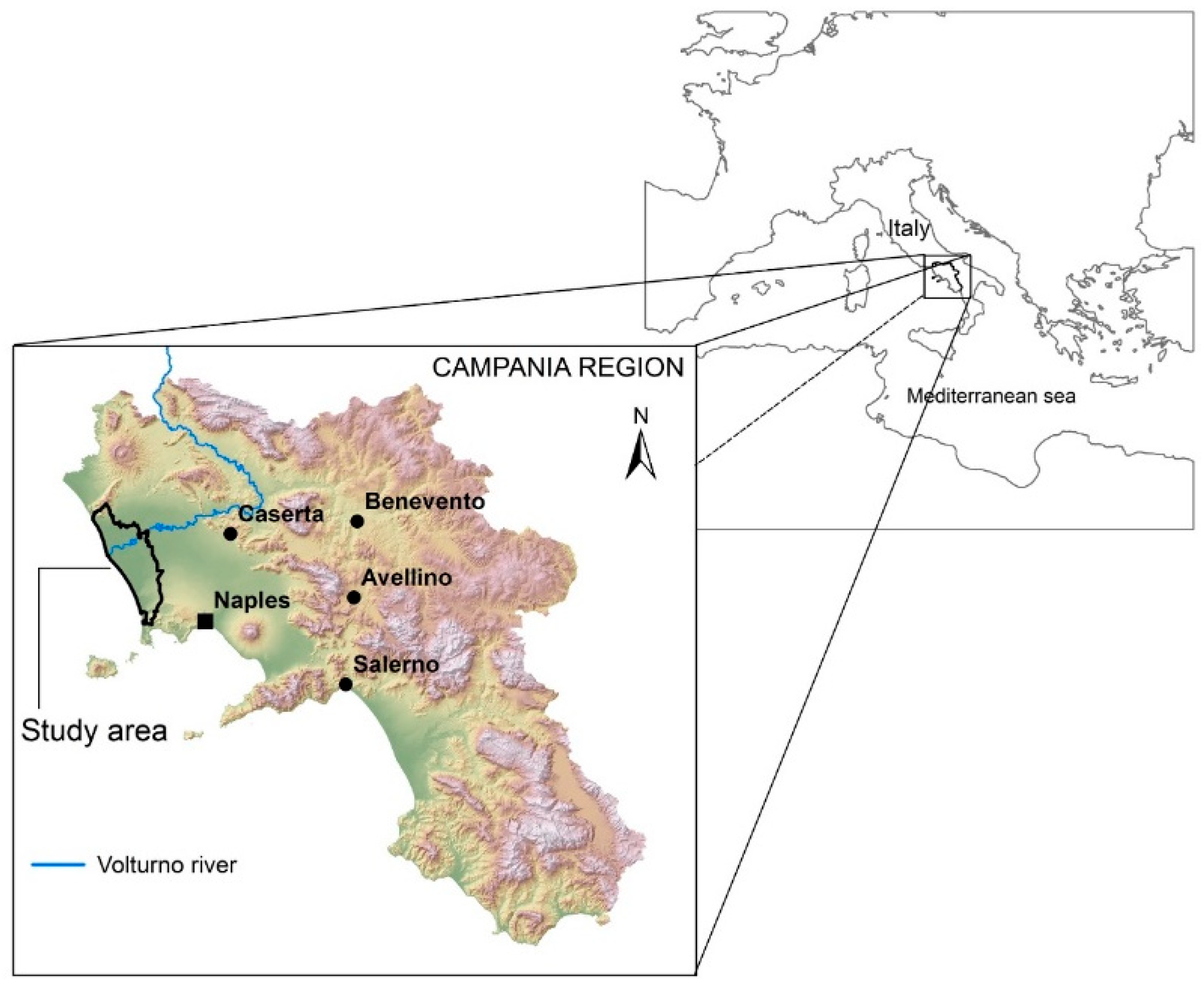
2.1. Study Area

The study area (Figure 1) is located to the north-western part of the Campania Region, in southern Italy (Coord. 41°01′00″ N, 13°58′00″ E). The climate shows characteristics typical of the Mediterranean region, with the wettest period between late autumn (October–November) and early spring (March–April).

Temperature and reference evapotranspiration are inversely related to rainfall, with the highest values during summer (June–August). According to Köppen classification [29], the climate subtype is “Csa—Hot-summer Mediterranean Climate”. The coastal belt of the lower Volturno river basin is a rich agricultural land, mainly devoted to irrigated vegetal crops and fruit trees [30]. The dominant soils are Gleyic, Gleyic-Vertic, Calcari-Gleyic and Calcari-Fluvic Cambisols, and CalcaricGleysols [31].

2.2. Soil Sampling and Analyses

For the purpose of this study, an existing soil database, available at the Institute for Agricultural and Forestry Systems in the Mediterranean of the National Research Council of Italy (CNR-ISAFoM), was used. This database contains information on soil organic carbon (OC), particle size distribution (sand, silt and clay), and volumetric water retention (cm³ water cm⁻³ soil) at both FC (θwt −33 KPa) and PWP (θwt −1500 KPa). Information about OC was available for 96 samples, while those for sand, silt and clay contents and for FC and PWP were available only for 82 samples, which are part of the 96. The analytical data included surface soil samples randomly collected in 1999 within the study area, air-dried and ground to a size fraction passing a 2 mm sieve. Soil organic carbon and texture were determined according to the Italian Official Methods for Soil Analysis [32]. Namely, total clay (soil separate with <0.002 mm particle diameter) and silt (soil separate with 0.002 to 0.05 mm particle diameter) contents were determined with the pipet method. Total sand content (soil separate with 0.05 to 2.0 mm particle diameter) was determined by wet sieving; OC content was determined using Walkley-Black methods. Water retention at FC (θwt at −33 KPa) and PWP (θwt at −1500 KPa) was measured with a Richards pressure, according to the Italian Methods of Physical Analysis of Soils [33], on undisturbed soils, taken in a ring core of a height of 5 cm and a diameter of 6.8 cm.

2.3. Statistical Analysis of Soil Properties

All basic (OC, sand, silt and clay contents) and hydraulic (FC and PWP) soil variables were statistically described in terms of minimum, maximum, mean, coefficient of variation (CV), and skewness. Before further statistical analyses, a log-transformation was performed for those variables that did not follow a normal distribution. Relationships among the variables were investigated using Pearson’s correlation coefficients. The XLStat statistical software, ver. 6.5 was used to this end.

2.4. Vis-NIR Spectroscopy

The diffuse vis-NIR reflectance was measured in the laboratory, on a residual fraction of the air-dried and 2 mm-sieved soil samples previously used for chemical and hydraulic analyses. Prior to spectral measurements, the samples were oven-dried at 40 °C during 12 h, in order to eliminate any possible residual moisture; then each sample was further grounded to minimize anisotropic scattering. The spectral measurements were carried out using a FieldSpec Pro spectroradiometer (Analytical Spectral Devices Inc, Boulder, CO, United States, 2013), with the help of a high-intensity contact probe (also from Analytical Spectral Devices) that uses a halogen bulb (2901 Å} 10 K) for illumination. The FieldSpec Pro spectroradiometer combines three spectrometers to cover the portion of the spectrum between 350 and 2500 nm. The instrument has a spectral sampling distance of ≤1.5 nm for the 350–1000 nm region and 2 nm for the 1000–2500 nm region. The contact probe measures a spot of diameter 10 mm, and it is designed to minimize errors associated with stray light. The sensor was calibrated with a Spectralon^® white reference panel. For each soil sample, four spectra were averaged to minimize noise and so to maximize the signal-to-noise ratio. Noisy portions of the spectra between 350 and 399 nm and between 2451 and 2500 nm were removed, leaving spectra in the range of 400–2450 nm for the analysis.

The continuum removal approach [34] was used to normalize the reflectance spectra for comparing absorption features from a common baseline. The continuum can be calculated using different functions. In this work, a convex hull was fitted over the original spectral curve, then the absorption spectrum was calculated by taking the ratio between the original reflectance spectrum and the enveloping curve [35,36].

2.5. Multivariate Calibration

Multivariate calibrations were performed to predict the investigated soil properties from reflectance spectra, using the software ParLeS [37]. PLSR was used to calibrate the spectral data with the reference (laboratory) soil data using two-thirds of the available samples for calibration and the remaining third to independently validate them. For each variable, the selection of samples was carried out as follows: First, the samples were sorted following ascending order of the variable, then, sequentially, every two samples were taken for calibration and the third for validation.

To enhance the predictive power of multivariate calibration models, spectroscopic data were transformed and pre-processed prior to data analysis, with the aim of removing undesired variation in the data [38]. In this study, we assessed all the transformation and pre-processing methods, either alone or in combination, before multivariate calibration. These methods include multiplicative scatter correction (MSC) [39], standard normal variance (SNV) correction [40,41], wavelet detrending (WD) [42], first and second derivative transformation, median [37], and Savitzky-Golay filtering [43].

Before multivariate modelling, spectra were also pre-treated by mean centering the data. The above procedures were applied alternatively to the original reflectance spectra (R) and to their absorbance (A = log 1/R).

Leave-one-out cross-validation [44] was then used to determine the number of factors to retain in the calibration models. To select the optimal cross-validated calibration model, we computed the root mean squared error (RMSE) of predictions:

$$\mathrm{RMSE}=\sqrt{\frac{1}{\mathrm{N}}{\displaystyle \sum }_{\mathrm{i}=1}^{\mathrm{N}}{(y_{pred}-y_{ob})}^2}$$

(1)

where N is the sample population size, y_pred is the predicted value, and y_ob is the observed value. The model with the lowest RMSE is usually selected. However, a more parsimonious PLSR model, i.e., a model with fewer factors, that represents the variability in the data without causing it to overfit, is better to use. To this end, the optimal selection of factors can be based on the Akaike Information Criterion (AIC) [45,46]:

AIC = Nlog (RMSE) + 2 m

(2)

where N is the sample population size, and m is the number of model parameters (i.e., the number of factors). To evaluate the accuracy of models, the adjusted coefficient of determination (R²adj) and the relative per cent deviation (RPD), that is the ratio of the standard deviation of analyzed data (i.e., the soil properties) to RMSE, was used.

In accordance with previous studies [47,48], the quality of predictions expressed by RPD was classified as follows: RPD <1.0 indicates very poor model/predictions and their use is not recommended; RPD between 1.0 and 1.4 indicates poor model/predictions where only high and low values are distinguishable; RPD between 1.4 and 1.8 indicates fair model/predictions which may be used for assessment and correlation; RPD values between 1.8 and 2.0 indicate good model/predictions where quantitative predictions are possible; RPD between 2.0 and 2.5 indicates very good, quantitative model/predictions; and RPD > 2.5 indicates excellent model/predictions.

We also used the R²adj and RPD statistics to assess the performance of validation, using the independent data set.

3. Results and Discussions

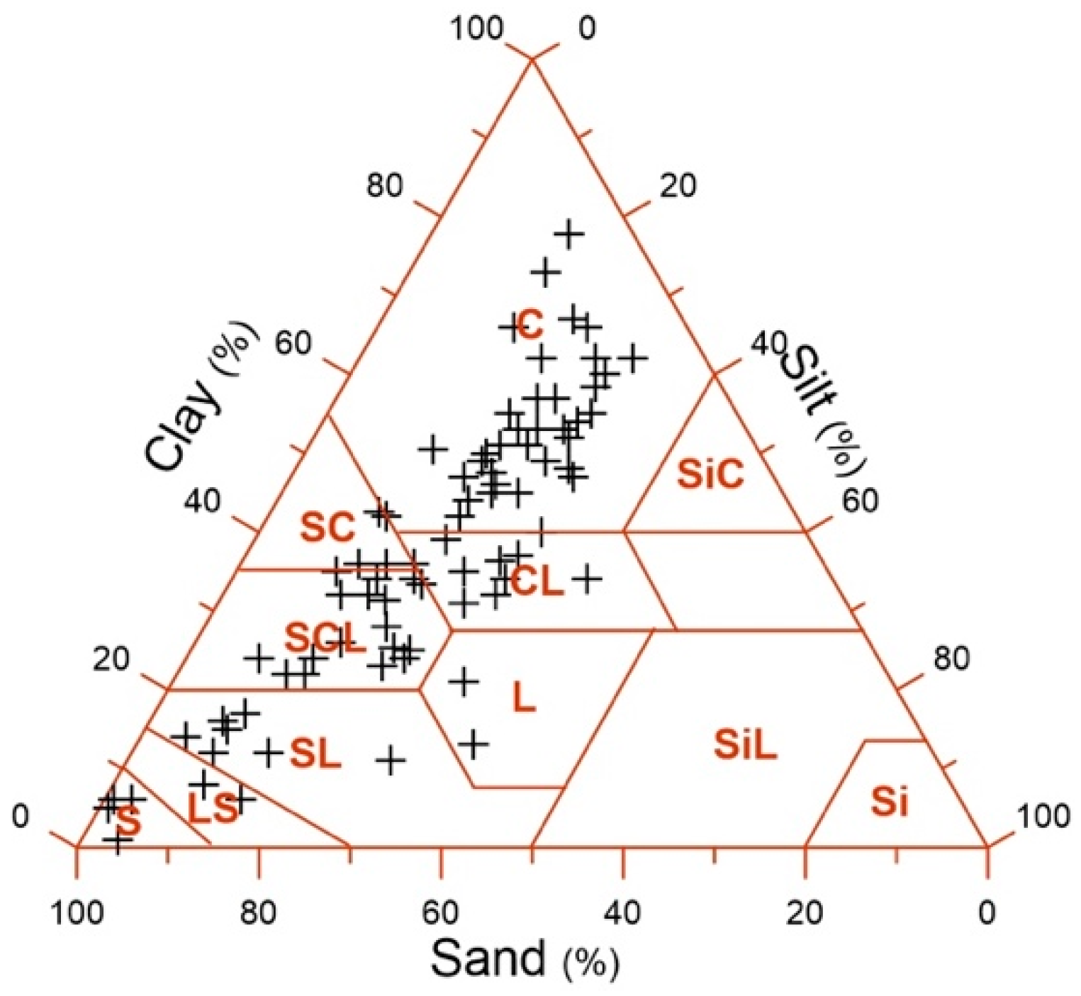
3.1. Soil Properties

Summary statistics, calibration and validation subsets are provided in

Table 1. Descriptive statistics of the selected soil properties for both calibration and validation data.

		n	Mean	Range	CV	Skewness
OC (g kg−1)	Calibration	64	22.5	4.4–215.6	1.43	4.52
	Validation	32	19.6	2.8–121.4	1.12	3.74
	All data	96	21.5	2.8–215.6	1.35	4.57
Sand (g kg−1)	Calibration	54	419.8	80.0–940.0	0.53	0.59
	Validation	28	423.6	70.0–950.0	0.56	0.64
	All data	82	421.1	70.0–950.0	0.54	0.60
Silt (g kg−1)	Calibration	54	201.1	10.0–370.0	0.39	−0.35
	Validation	28	201.1	10.0–390.0	0.43	−0.23
	All data	82	201.1	10.0–390.0	0.40	−0.30
Clay (g kg−1)	Calibration	54	377.4	50.0–730.0	0.46	−0.14
	Validation	28	378.9	10.0–770.0	0.50	−0.09
	All data	82	377.7	10.0–770.0	0.47	−0.12
FC (m3 m−3)	Calibration	54	0.33	0.07–0.60	0.36	0.19
	Validation	28	0.34	0.07–0.56	0.35	−0.06
	All data	82	0.33	0.07–0.60	0.36	0.10
PWP (m3 m−3)	Calibration	54	0.21	0.05–0.42	0.38	0.36
	Validation	28	0.21	0.04–0.45	0.43	0.49
	All data	82	0.21	0.04–0.45	0.43	0.41

. Organic carbon content is on average moderate (21.5 g kg⁻¹), but highly variable (CV 1.35), within a range from 2.71 to 215.6 g kg⁻¹. A slight difference in the average values exists between the calibration (22.5 g kg⁻¹) and validation (19.6 g kg⁻¹) sub-sets. Skewness exhibits always high values (4.47 for the whole data-set; 4.52 and 3.74 for the calibration and validation sub-stets, respectively), thus indicating a significant deviation from the normal distribution.

Sand was the dominant particle size fraction (421.1 g kg⁻¹, on average), followed by clay (377.7 g kg⁻¹) and silt (201.1 g kg⁻¹). The dominant soil texture (Figure 2) ranges from fine (clay), to moderately fine (clay-loam, sandy-clay-loam), to moderately coarse (sandy-loam). Mean and extreme values for all, sand, silt and clay calibration, and validation subsets are similar. Skewness was consistent, thus indicating, for these variables, a frequency distribution close to the normal distribution. Water retention at FC and PWP is, on average, 0.33 m³m⁻³ and 0.20 m³m⁻³, respectively. Differences between calibration and validation sub-sets are minimal, and the CV is moderate for both these variables. Skewness is consistently low. Considering that the mean and the coefficient of variation for the calibration and validation sets are comparable for all the basic and hydraulic soil properties, the selection of both datasets can be considered representative [49].

Significant correlations exist among the investigated soil variables (

Table 2. Correlation coefficients between the selected basic and hydraulic soil properties.

	OC	Sand	Silt	Clay	FC
Sand	−0.337 **
Silt	0.233 *	−0.691 ***
Clay	0.317 **	−0.942 ***	0.408 ***
FC	0.604 ***	−0.659 ***	0.473 ***	0.608 ***
PWP	0.615 ***	−0.679 ***	0.467 ***	0.639 ***	0.959 ***

p-values ≤ 0.05 (*), ≤0.001 (**), ≤0.0001 (***).

). As expected, the highest, negative correlation was between clay and sand contents. Of particular interest for the purposes of this study, were the correlations between OC, sand and clay contents, and the soil hydraulic properties.

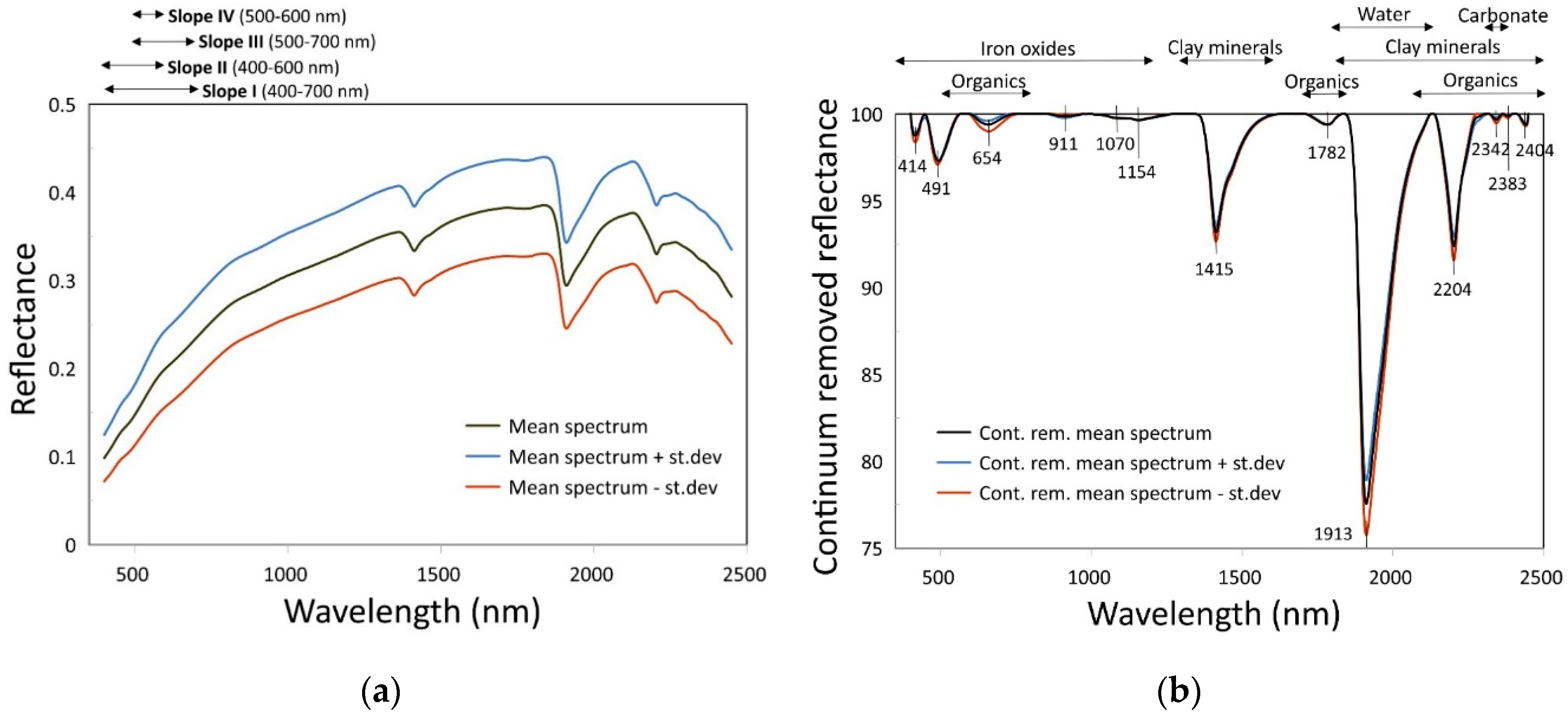
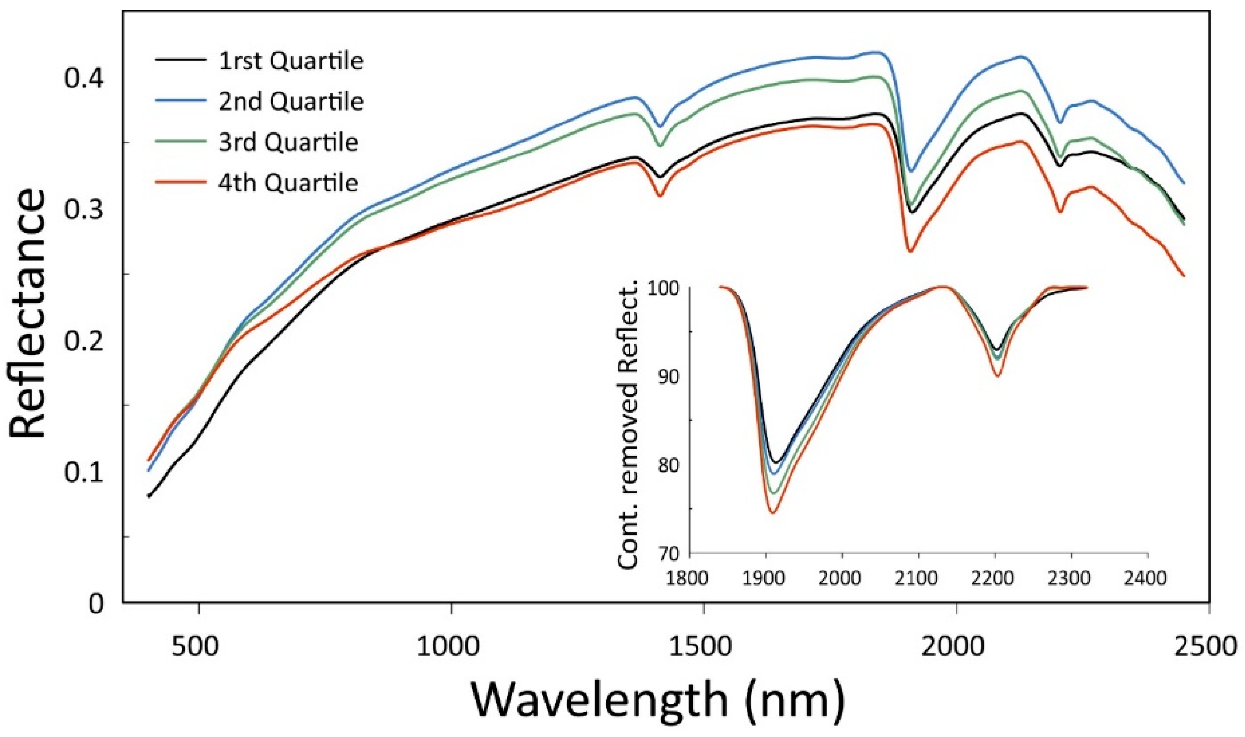
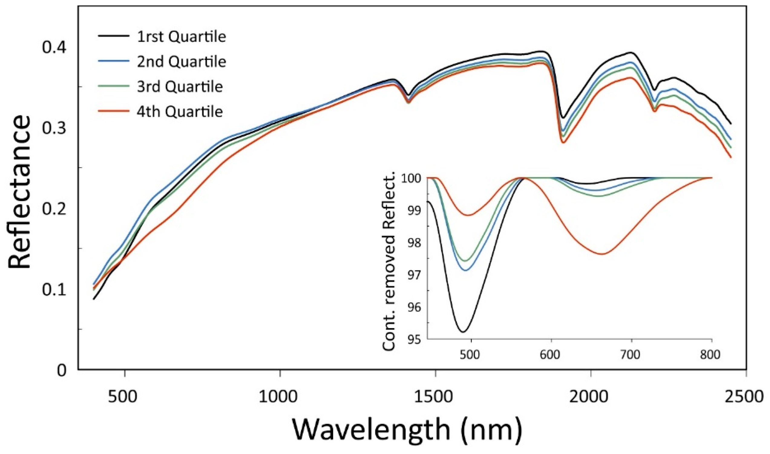
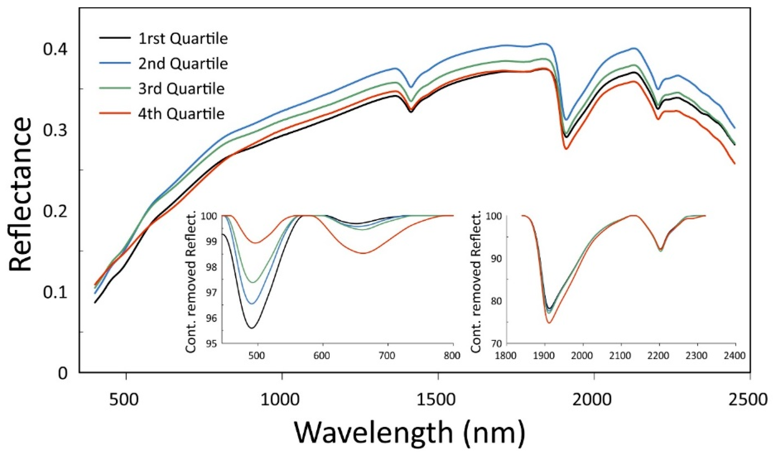
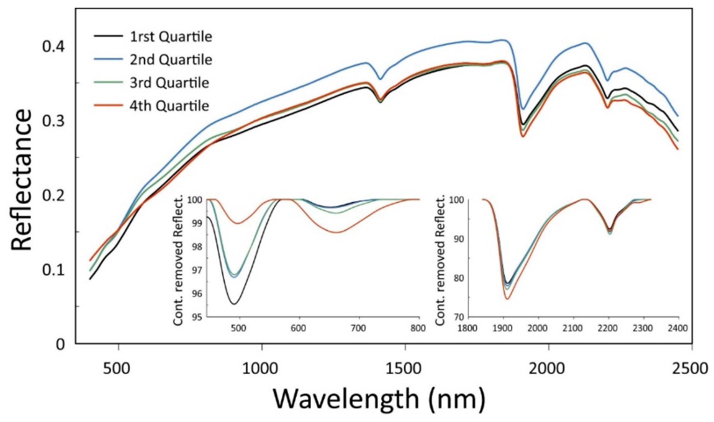
3.2. Soil Spectral Characteristics

Figure 3 shows the average soil spectrum and the relative continuum removed reflectance of the investigated soil samples and their standard deviation.

The average spectrum (Figure 3a) shows a typical convex shape and a moderate overall reflectance. The dispersion of the spectral intensity, as measured by the standard deviation, was evident. Many studies demonstrated that different soil properties, especially particle size distribution and organic carbon content, may affect the overall reflectance [24]. Changes in slopes of different ranges in the visible region are also observed. Various studies have related visible reflectance slopes to soil organic matter content [50]. The average continuum removed spectrum (Figure 3b) shows a number of absorption bands across the entire vis-NIR region, which can be related to clay minerals, organic matter, iron oxides, water, and carbonate contents [24,51].

In order to visually analyze the direct and indirect effects of the investigated basic and hydraulic soil properties on soil spectral reflectance, the mean spectra of quartiles for each of these properties were calculated [50]. Figure 4 shows the mean spectra of quartiles for clay content. Absorption bands near 1400, 1900 and 2200 nm are affected by clay minerals [22], and the absorption feature near 2200 nm is due to Al–OH bending, as in kaolinite, smectite and illite; that at 1400 nm can be attributed partly to an overtone of structural O–H stretching, as in kaolinite and illite, and partly to the combination vibrations in the water bond in the interlayer lattice, related to hydrate cations and water absorbed on particle surfaces. Absorptions by H₂O also cause the absorption band near 1900 nm [24].

Smectitic clays dominate the study area and the nature of the spectra support this, as shown by the presence of a shallow absorption band near 2200 nm (value <1 for asymmetry), and an intense absorption band near 1900 nm (Figure 4) [35,52]. Asymmetry is the ratio of the area-left to the area-right of the line through the center of an absorption feature. As expected, quartiles spectra for sand content (not shown) displayed an opposite trend, with respect to clay content (Table 2). No noteworthy relation was observed between the silt content and quartile spectra (not shown). Regression analysis (

Table 3. Regression coefficients between OC, water retention at the field capacity (FC) and permanent wilting point (PWP) and 1/slopes of reflectance spectra in different ranges ** of the visible wavelengths.

	Clay	OC *	FC	PWP
Slope I (400–700 nm)	–	0.398 (l)	0.199 (l)	0.204 (l)
Slope II (400–600 nm)	–	0.530 (l)	0.243 (l)	0.259 (l)
Slope III (500–700 nm)	–	0.270 (l)	0.202 (l)	0.196 (l)
Slope IV (500–600 nm)	–	0.580 (l)	0.310 (l)	0.317 (l)
Depth abs. band 660 nm	–	0.561 (ex)	0.171 (ex)	0.212 (ex)
Depth abs. band 1900 nm	0.417 (l)	–	0.244 (l)	0.296 (l)
Depth abs. band 2200 nm	0.681 (l)	–	0.147 (l)	0.157 (l)

* log₁₀ transformed, ^(l) linear regression; ^(ex) exponential regression. ** Spectral ranges correspond to those considered by [53].

) revealed positive linear relationships between clay content and depth of the absorption bands near 1900 nm (R² = 0.42) and near 2200 nm (R² = 0.68).

Figure 5 shows the mean soil spectra of the quartiles for OC. No trend with increasing OC content was observed in the visible, or the first section of the NIR ranges (Figure 5), which is probably due to the effects of other soil properties (i.e., texture, carbonates, iron-oxides at these ranges). On the other hand, a clear negative trend was observed in the longer wavelengths of the NIR range (1450–2450 nm). However, there was no significant relationship observed between OC content and the reflectance integrated (albedo) over the portion of spectra in this range. Some significant relationships were observed between OC and other spectral features, such as slopes and absorption bands in the visible range (Table 3). In particular, 1/slopes in the visible ranges 400–700 nm (Slope I), 400–600 nm (Slope II), 500–700 nm (Slope III), and 500–600 nm (Slope IV) [53], increased with OC content.

According to Ref. [53], the inverse values of slopes (1/slopes) were considered, instead of those of slopes, to make the regressions linear. The best linear regressions (Table 3) were those found between log-transformed OC and 1/Slope IV (500–600 nm) (R² = 0.580) and 1/Slope II (400–600 nm) (R² = 0.530). From Figure 5, it is evident that the depth of the absorption band near 650 nm (as observed on the continuum removed reflectance spectra) tends to increase with increasing OC. Ref. [21] reported that the band near 660 nm may be important for the prediction of OC. Ref. [23] attributed the absorption near 664 nm to pigment residuals in the soil organic matter. In this study, a moderate (R² = 0.561) exponential regression (Table 3) was found between the absorption depth at 650 nm and the log-transformed OC content. From Figure 4, it also appears that organic matter affects the absorption band depth near 480 nm. This was attributed to the influence of OC on the spectral absorption on iron-oxides in the visible and first range of NIR [54,55]. In particular, Goethite absorbs mostly near 480 nm, and the intensity of the absorbance at this wavelength is significantly masked by the optical interference of organic matter.

The characteristics of the mean spectra of quartiles for the FC (Figure 6) and PWP (Figure 7) reflect those of the mean spectra of quartiles for clay, sand (not shown) and OC.

In particular, as both FC and PWP increase, the relative depth of absorption bands near 1900 nm and 660 nm also increases, while the one near 480 nm decreases. In both the quartile spectra of FC and PWP, no trend was observed for the 2200 nm band. The 1/slopes of spectra in the visible ranges also decreased with increasing FC and PWP. However, in all cases (Table 3), the regression coefficients (R²) between both FC and PWP and the above spectral variables (depth of bands at 660 nm and 1900 nm, visible 1/slopes) were lower than those between the basic soil properties (particularly OC and clay contents) and the same spectral variable. On the basis of these results, it is reasonable to expect positive results from the subsequent multivariate calibration.

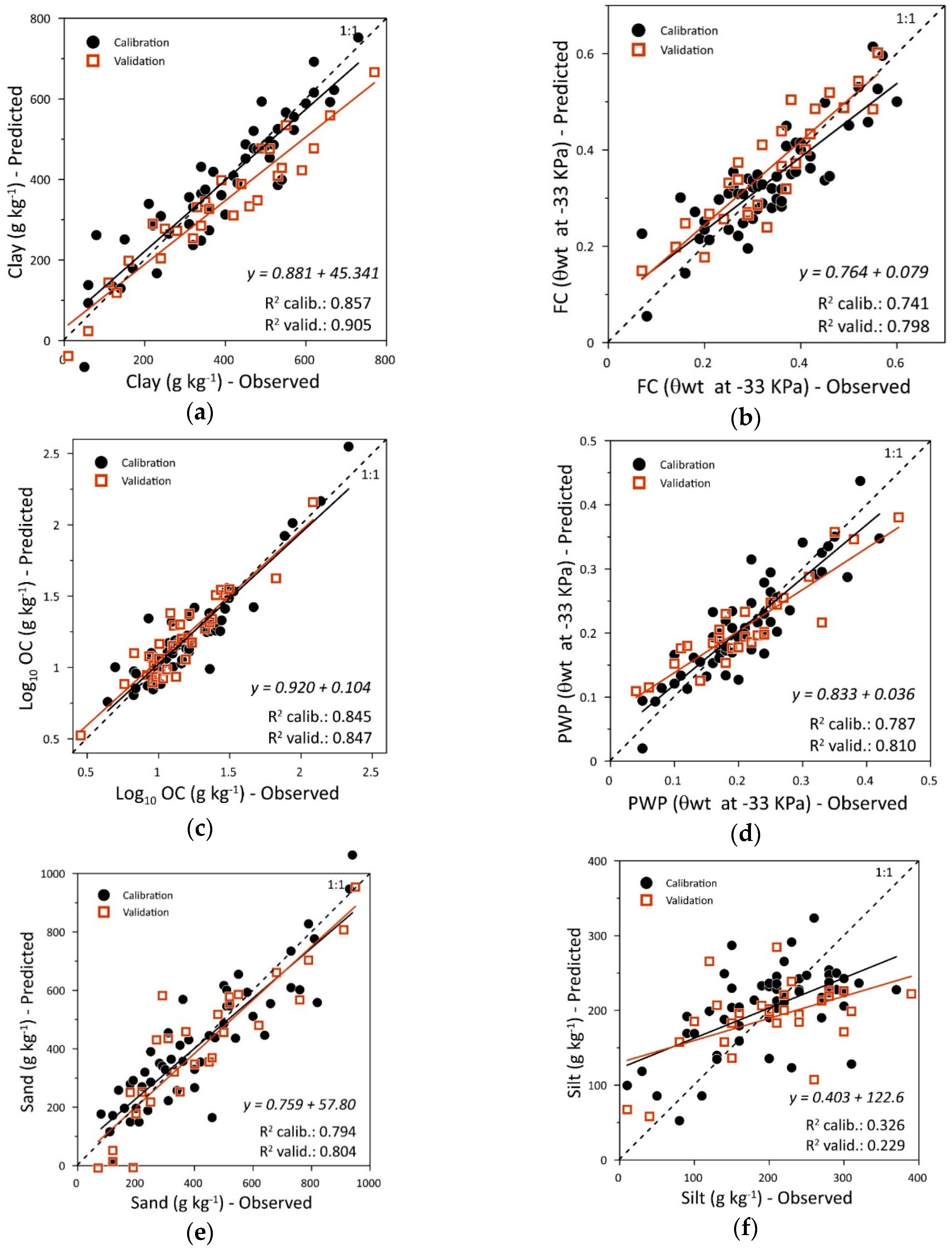
3.3. Multivariate Calibration

The ability of vis-NIR reflectance spectroscopy to predict the investigated hydraulic and basic soil properties is summarized in

Table 4. Results of PLSR applied to basic and hydraulic soil properties and soil spectral reflectance in the vis-NIR spectral domain.

Soil Property	Calibration				Validation
	n. Fact.	R2adj	RMSE	RPD	R2adj	RMSE	RPD
OC *	8	0.845	0.124	2.52	0.847	0.122	2.50
Sand	7	0.794	100.71	2.22	0.804	106.37	2.24
Silt	4	0.326	64.40	1.23	0.229	74.38	1.16
Clay	5	0.857	64.80	2.69	0.905	56.71	3.33
FC	5	0.741	0.060	2.00	0.798	0.048	2.05
PWP	5	0.787	0.038	2.20	0.810	0.044	2.18

* log₁₀ transformed.

. Scatterplots of the predicted vs measured values for these properties are shown in Figure 8. The best results were achieved by pre-processing the spectra prior to data analysis by applying a combination of the following procedures: reflectance (R) to absorbance (A) transformation (A = log 1/R), wavelet detrending, Savitzly-Golay filtering, second derivative of absorbance, and data enhancement (mean centre). Reflectance to absorbance transformation reduces nonlinearities [37], while wavelet detrending [42] corrects light scattering variation and baseline. The Savitzky-Golay filter [43] (carried out prior to the second derivative transformation) reduces the effects of spectral random noise, thereby providing smoother spectra. The second derivative removes additive and linear baseline effects [56], while amplifying absorption features, which are indicative of the contents of the soil materials. Mean centering is a commonly used method of data enhancement to reduce redundant information.

PLSR applied to the two-thirds of the available sample set provided good correlations between soil spectra and the selected soil properties, except for silt. Based on the values of RPD, the calibration models were excellent for clay (RPD 2.69) and log-OC (RPD 2.52) and very good for sand (RPD 2.22), FC (RPD 2.00) and PWP (RPD 2.20). For clay, FC and PWP, models including five factors (based on the RMSE and AIC values) allowed to achieve a cross-validation between predicted and measured data with R²adj of 0.857, 0.741 and 0.787, respectively. For log-OC and sand (models with a higher number of factors; 8 and 7, respectively) cross-validation resulted in an R²adj of 0.845 and 0.794, respectively. For silt, it was possible to calibrate only a poor model, with an R²adj of 0.326 and RPD of 1.23. In some cases, increasing the number of factors gave slightly higher coefficients of regression (R²), but increased RMSE, thus reducing the stability of the calibration models (i.e., leading to over-fitting) [57,58]. Therefore, we selected the most parsimonious model, in terms of number of factors, based on the values of AIC and RMSE. Leave-one-out calibration models constructed through vis-NIR reflectance spectroscopy and PLSR are empirical; therefore, validations of these models are better performed using a data set that is independent of the one used for calibration [59].

Validation using the remaining one-third of the available samples indicated excellent models for the prediction of clay (R²adj 0.905 and RPD 3.33) and log-OC (R²adj 0.847 and RPD 2.50); very good models for sand (R²adj 0.804 and RPD 2.24), PWP (R²adj 0.810 and RPD 2.18) and FC (R²adj 0.798 and RPD 2.05); and a poor model for silt (R²adj 0.229 and RPD 1.16).

The predictions obtained from the present investigation (Table 4 and Figure 8), using PLSR and vis-NIR spectroscopy, are consistent with similar predictions in other geographical areas of the world and in some cases better. For instance, in a study of reflectance spectroscopy for the prediction of field capacity, PWP and other soil properties, Ref. [60] found values of R² and RPD of 0.79 and 1.93, respectively, for the prediction of FC and of 0.80 and 2.18, for the prediction of PWP, in agreement with the results of our research. Our results agree with these observations. In contrast with our finding, the same authors were able to calibrate models for sand, silt and clay. The prediction of OC (R² = 0.87) is in agreement with other studies: Ref. [59] (R² = 0.84), working on soil samples from Mollic Ustifluvent, Typic Ustifluvent and Typic Ustorthent of a semi-arid environment of northern Turkey; Ref. [27] (R² = 0.83), working on soils from different sites of the Armorican Massif, Brittany region, France; and Ref. [61] (R² = 0.91), working on soils from the Kakamega Forest, Kenya. Predictions comparable with our results, were previously achieved by Refs. [62] (R² = 0.69/0.88), [63] (R² = 0.85) and [64] (R² = 0.89), who used soil samples from the Trier region, south Germany, west-central United States, and various areas of Iowa and Minnesota, USA, respectively. Our prediction of OC resulted much better than those found by Refs. [21] (R² = 0.60; soils from Kelso New South Wales, Australia), [65] (R² = 0.70; soils from the Liverpool plain, New South Wales), [66] (R² = 0.60; soils from the Bakenhof flood, The Netherlands), and [67] (R² = 0.66; soils from Southern NSW, Australia). In our opinion, the reasons for these discrepancies are in the specificity of the different pedo-environments.

The predictions of sand and clay are in a good agreement with those from the works of Refs. [59,68] (R² = 0.84 and 0.88, for sand and clay, respectively) and [69] (R² = 0.88 for clay) and with the work of Ref. [70] (R² = 0.91) on soils from different region of Denmark. Instead, they were much better than those from the work of Refs. [69] (R² = 0.88 for sand), [21] (R² = 0.47/0.59 e 0.43/0.60 for sand and clay, respectively) and [61] (R² = 0.75 and 0.77 for sand and clay, respectively).

4. Conclusions

This study focused on the use of vis-NIR reflectance spectroscopy under controlled laboratory conditions for characterizing hydraulic (water retention at the FC and PWP) and related, basic soil properties (clay, sand, silt and organic carbon contents) in the coastal area of the lower Volturno river basin, southern Italy.

All basic soil properties, with the exception of silt, were significantly correlated with FC and PWP. Visual analysis of reflectance spectra showed that both clay and organic matter evidently affect some specific spectral features, such as absorption depth at 1900 and 2200 nm (clay), absorption at 650 nm, and spectra slopes in the visible region (OC). The presence of OC weakens the absorption of iron-oxides near 480 nm. Sand, being inversely and significantly related to clay, shows an opposite effect on reflectance spectra, compared to that of clay. Any visual influence of silt on the spectral reflectance was not observed. Giving their positive correlations with OC, clay and sand, both FC and PWP indirectly affected most of the above-mentioned spectral features. Regression analysis quantitatively corroborated most of the relationships between spectral features and both basic and hydraulic soil properties. Using PLSR, it was possible to calibrate and validate very good models for the prediction of FC, PWP and sand and an excellent model for OC and clay.

PLSR was used to predict water retention at FC and PWP as well as sand, clay and organic carbon content. Excellent predictions were obtained for clay and organic carbon, and those for sand, FC and PWP were very good, whereas prediction for silt was poor. As a result, the mathematical equations identified in this study, based on laboratory reflectance measurements, can be used to determine, in a simple and relatively inexpensive way, the considered soil properties, with the exception of silt.

Furthermore, vis-NIR reflectance spectroscopy is a rapid technique, making it possible to analyze a large number of samples in a practical and timely manner. The results achieved in this study, although promising, need to be further validated in the whole irrigation territory of the lower Volturno river basin and other irrigation districts of Italy characterized by different pedo-environments.

It might be desirable to assess the potential of the reflectance spectroscopy in the prediction of the considered soil properties using field measurements. However, the spatial variability of the physical conditions of the soils in the field (humidity, stoniness, particles aggregation) could significantly affect the spectral response of the soil fine earth fraction, thus interfering with the quality of prediction models. The evaluation of these effects will be one of the objectives of future research activities.

References

1. Zucaro, R. Atlas of Italian Irrigation Systems; Centro Stampa e Riproduzione: Rome, Italy, 2014; p. 174. [Google Scholar]
2. International Commission on Irrigation and Drainage. Available online: https://www.icid.org/v_italy.pdf (accessed on 25 July 2019).
3. Alvino, A.; Marino, S. Remote Sensing for Irrigation of Horticultural Crops. Horticulturae 2017, 3, 40. [Google Scholar] [CrossRef]
4. Abbasi, Y.; Ghanbarian-Alavijeh, B.; Liaghat, A.M.; Shorafa, M. Evaluation of pedotransfer functions for estimating soil water retention curve of saline and saline-alkali soils of Iran. Pedosphere 2011, 2, 230–237. [Google Scholar] [CrossRef]
5. White, R.E. Principles and Practices of Soil Science; Blackwell Publishing: Padstow, Cornwall, UK, 2006; p. 363. [Google Scholar]
6. Silva, B.M.; da Silva, É.A.; de Oliveira, G.C.; Ferreira, M.M.; Serafim, M.E. Plant-available soil water capacity: Estimation methods and implications. Rev. Bras. Cienc. Solo 2014, 38, 464–475. [Google Scholar] [CrossRef]
7. Ferreira, M.I. Stress Coefficients for Soil Water Balance Combined with Water Stress Indicators for Irrigation Scheduling of Woody Crops. Horticulturae 2017, 3, 38. [Google Scholar] [CrossRef]
8. White, R.E. Soils for Fine Wines; Oxford University Press: Oxford, NY, USA, 2003; p. 279. [Google Scholar]
9. Brady, N.C.; Weil, R.R. The Nature and Properties of Soils; Prentice Hall: Upper Saddle River, NJ, USA, 2002; p. 960. [Google Scholar]
10. Vereecken, H.; Weynant, M.; Javaux, M.; Pachepsky, Y.; Schaap, M.G.; van Genuchten, M.T. Using pedotransfer functions to estimate the van Genuchten-Maulem soil hydraulic properties. A review. Vadose Zone J. 2010, 9, 1–26. [Google Scholar] [CrossRef]
11. Leone, A.P.; Viscarra-Rossel, A.R.; Amenta, P.; Buondonno, A. Prediction of soil properties with PLSR and vis-NIR spectroscopy: Application to Mediterranean soils from Southern Italy. Curr. Anal. Chem. 2012, 8, 283–299. [Google Scholar] [CrossRef]
12. Haghverdi, A.; Ozturk, H.S.; Cornelis, W.M. Revisiting the pseudo continuous pedotransfer function concept: Impact of data quality and data mining method. Geoderma 2014, 226, 31–38. [Google Scholar] [CrossRef]
13. Bouma, J. Using soil survey data for quantitative land evaluation. Adv. Soil Sci. 1989, 9, 177–213. [Google Scholar]
14. Vereecken, H.; Maes, J.; Feyen, J.; Darius, P. Estimating the soil-moisture retention characteristic from texture, bulk density, and carbon content. Soil Sci. 1989, 148, 389–403. [Google Scholar] [CrossRef]
15. Tomasella, J.; Hodnett, M.G. Estimating soil water retention characteristics from limited data in Brazilian Amazonia. Soil Sci. 1998, 163, 190–202. [Google Scholar] [CrossRef]
16. Zhao, C.; Shao, M.; Jia, X.; Nasir, M.; Zhang, C. Using pedotransfer functions to estimate soil hydraulic conductivity in the Loess Plateau of China. Catena 2016, 143, 1–6. [Google Scholar] [CrossRef]
17. Dobarco, M.R.; Cousin, I.; Le Bas, C.; Martin, M. Pedotransfer functions for predicting available water capacity in French soils, their applicability domain and associated uncertainty. Geoderma 2019, 336, 81–95. [Google Scholar] [CrossRef]
18. Ben-Dor, E.; Irons, J.R.; Epema, G.F. Soil reflectance. In Remote Sensing for the Earth Sciences: Manual of Remote Sensing, 3rd ed.; Rencz, A.N., Ed.; Wiley: New York, NY, USA, 1999; Volume 3, pp. 111–188. [Google Scholar]
19. Drury, S.A. Image Interpretation in Geology; Chapman & Hall: London, UK, 1993; p. 283. [Google Scholar]
20. Milton, E.J. Principles of field spectroscopy. Int. J. Remote Sens. 1987, 12, 1807–1827. [Google Scholar] [CrossRef]
21. Viscarra Rossel, R.A.; Walvoort, D.J.J.; McBratney, A.B.; Janik, L.J.; Skjemstad, J.O. Visible, near infrared, mid infrared or combined diffuse reflectance spectroscopy for simultaneous assessment of various soil properties. Geoderma 2006, 131, 59–75. [Google Scholar] [CrossRef]
22. Marino, S.; Aria, M.; Basso, B.; Leone, A.P.; Alvino, A. Use of soil and vegetation spectroradiometry to investigate crop water use efficiency of a drip irrigated tomato. Eur. J. Agron. 2014, 59, 67–77. [Google Scholar] [CrossRef]
23. Ben-Dor, E.; Inbar, Y.; Chen, Y. The reflectance spectra of organic matter in the visible near-infrared and short wave infrared region (400–2500 nm) during controlled decomposition process. Remote Sens. Environ. 1997, 61, 1–15. [Google Scholar] [CrossRef]
24. Stenberg, B.; Viscarra Rossel, R.A.; Mouazen, A.M.; Wetterlind, J. Visible and near infrared spectroscopy in soil science. In Advances in Agronomy; Sparks, D.L., Ed.; Academic Press: Burlington, VT, USA, 2010; Volume 107, pp. 163–215. [Google Scholar]
25. Babaeian, E.; Homaee, M.; Vereeckem, H.; Montzka, C.; Norouzi, A.A.; van Genuchten, M.T. A Comparative Study of Multiple Approaches for Predicting the Soil–Water Retention Curve: Hyperspectral Information vs. Basic Soil Properties. Soil Sci. Soc. Am. J. 2015, 79, 1043–1058. [Google Scholar] [CrossRef]
26. Sudduth, K.A.; Hummel, J.W. Soil organic matter, CEC and moisture sensing with a portable NIR spectrophotometer. Trans. ASAE 1993, 36, 1571–1582. [Google Scholar] [CrossRef]
27. Aïchi, H.; Fouad, Y.; Walter, C.; Viscarra Rossel, R.A.; Chabaane, Z.L.; Sanaa, M. Regional predictions of soil organic carbon content from reflectance measurements. Biosyst. Eng. 2009, 104, 442–446. [Google Scholar] [CrossRef]
28. Ingleby, H.R.; Crowe, T.G. Neural network models for predicting organic matter content in Saskatchewan soils. Can. Biosyst. Eng. 2001, 43, 3. [Google Scholar]
29. Köppen, W.P. Handbuch Der Klimatologie. Das Geographisca System Der Klimate. In Handbuch Der Klimatologie; Köppen, W., Geiger, G., Eds.; C. Borntraeger Science Publishers: Stuttgart, Germany, 1930; Volume 1, p. 44. [Google Scholar]
30. Geoportale Regione Campania. Sistema Informativo Territoriale della Regione Campania. Available online: https://sit2.regione.campania.it/content/carta-utilizzazione-agricola-dei-suoli (accessed on 10 February 2019).
31. Di Gennaro, A. I sistemi di terra della Campania; SELCA: Florence, Italy, 2002; p. 63. [Google Scholar]
32. MIPAF (Ministero delle Politiche Agricole e Forestali). Metodi di Analisi Chimica del Suolo; Franco Angeli: Milan, Italy, 2000; p. 536.
33. MIPAF (Ministero delle Politiche Agricole e Forestali). Metodi di Analisi Fisica del Suolo; Franco Angeli: Milan, Italy, 1998; p. 400.
34. Clark, R.N.; Roush, T.L. Reflectance spectroscopy: Quantitative analysis techniques for remote sensing applications. J. Geophys. Res. 1984, 89, 6329–6340. [Google Scholar] [CrossRef]
35. Van der Meer, F. Can we map swelling clays with remote sensing? Int. J. Appl. Earth Obs. Geoinf. 1999, 1, 27–35. [Google Scholar] [CrossRef]
36. De Jong, S. The anaysis of spectroscopical data to map soil types and soil crusts of Mediterraneas eroded soils. Soil Technol. 1992, 5, 199–211. [Google Scholar] [CrossRef]
37. Viscarra Rossel, R.A. ParLeS: Software for chemometric analysis of spectroscopic data. Chemom. Intell. Lab. Syst. 2008, 90, 72–83. [Google Scholar] [CrossRef]
38. Eriksson, L.; Johansson, E.; Kettaneh-Wold, N.; Trygg, J.; Wilström, C.; Wold, S. Multi-and Megavariate Data Analysis; Part I-Basic principles and applications; Umetrics Academy: Umeå, Sweden, 2006; p. 425. [Google Scholar]
39. Geladi, P.; MacDouglas, D.; Martens, H. Linearization and scatter-correction for near-infrared reflectance spectra of meat. Appl. Spectrosc. 1985, 3, 491–500. [Google Scholar] [CrossRef]
40. Barnes, R.J.; Dhanoa, M.S.; Lister, S.J. Standard normal variate transformation and de-trending of near-infrared diffuse reflectance spectra. Appl. Spectrosc. 1989, 43, 772–777. [Google Scholar] [CrossRef]
41. Dhanoa, M.S.; Lister, S.L.; Sanderson, R.; Barnes, R.J. The link between multiplicative scatter correction (MSC) and standard normal variate (SNV) transformation of NIR spectra. J. Near Infrared Spec. 1994, 2, 43–47. [Google Scholar] [CrossRef]
42. Daubechies, I. Ten Lectures on Wavelets; Society for Industrial and Applied Mathematics: Philadelphia, PA, USA, 1992; p. 341. [Google Scholar]
43. Savitzky, A.; Golay, M.J.E. Smoothing and differentiation of data by simplified least squares procedures. Anal. Chem. 1964, 36, 1627–1639. [Google Scholar] [CrossRef]
44. Efron, B.; Tibshir, R.J. An Introduction of the Bootstrap, 1st ed.; Chapman and Hall: New York, NY, USA, 1993; p. 436. [Google Scholar]
45. Akaike, H. Fitting Autoregressive Models for Prediction. Ann. Inst. Stat. Math. 1969, 21, 243–247. [Google Scholar] [CrossRef]
46. Li, B.; Morris, J.; Martin, E.B. Model selection for partial least squares regression. Chemom. Intell. Lab. Syst. 2002, 1, 79–89. [Google Scholar] [CrossRef]
47. Williams, P.C. Variables affecting near-infrared reflectance spectroscopic analysis. In Near-Infrared Technology in the Agricultural and Food Industries; Williams, P.C., Norris, K., Eds.; American Association of Cereal Chemists Inc.: St. Paul, MN, USA, 1987; pp. 143–167. [Google Scholar]
48. Viscarra Rossel, R.A. Robust modelling of soil diffuse reflectance spectra by bagging-partial least squares regression. J. Near Infrared Spec. 2007, 15, 39–47. [Google Scholar] [CrossRef]
49. Ding, J.; Yang, A.; Wang, J.; Sagan, V.; Yu, D. Machine-learning-based quantitative estimation of soil organic carbon content by VIS/NIR spectroscopy. Peer J. 2018, 5714, 1–14. [Google Scholar] [CrossRef]
50. Summers, D.; Lewis, M.; Ostendorf, B.; Chittleborough, D. Visible near-infrared reflectance spectroscopy as a predictive indicator of soil properties. Ecol. Indic. 2011, 11, 123–131. [Google Scholar] [CrossRef]
51. Leone, A.P. Spettrometria e valutazione della riflettanza spettrale dei suoli nel dominio ottico 400–2500 nm. Riv. Ital. Telerilevamento 2000, 9, 3–28. [Google Scholar]
52. Kariuki, P.C.; Wolday, T.; Van der Meer, F. Effectiveness of spectroscopy in identification of swelling indicator clay minerals. Int. J. Remote Sens. 2004, 2, 455–469. [Google Scholar] [CrossRef]
53. Bartholomeus, H.M.; Schaepman, M.E.; Kooistra, L.; Stevens, A.; Hoogmoed, W.B.; Spaargaren, O.S.P. Spectral reflectance based indices for soil organic carbon quantification. Geoderma 2008, 145, 28–36. [Google Scholar] [CrossRef]
54. Henderson, T.L.; Baumgardner, M.F.; Franzmeier, D.P.; Stott, D.E.; Coster, D.C. High dimensional reflectance analysis of soil organic matter. Soil Sci. Soc. Am. J. 1992, 56, 865–872. [Google Scholar] [CrossRef]
55. Galvao, L.S.; Vitorello, I. Role of organic matter in obliterating the effects of iron on spectral reflectance and color of Brazilian tropical soils. Int. J. Remote Sens. 1998, 19, 1969–1979. [Google Scholar] [CrossRef]
56. Burger, J.; Geladi, P. Spectral pre-treatments of hyperspectral near infrared images: Analysis of diffuse reflectance scattering. J. Near Infrared Spec. 2007, 15, 29–37. [Google Scholar] [CrossRef]
57. Wise, B.M.; Gallagher, N.B.; Bro, R.; Shaver, J.M. PLS Toolbox Version 3.0 for Use with Matlab; Eigenvector Research Inc.: Wenatchee, WA, USA, 2003; p. 171. [Google Scholar]
58. Vågen, T.G.; Shepherd, K.D.; Walsh, M.G. Sensing landscape level change in soil fertility following deforestation and conversion in the highlands of Madagascar using Vis-NIR spectroscopy. Geoderma 2006, 133, 281–294. [Google Scholar] [CrossRef]
59. Volkan Bilgili, A.; van Es, H.M.; Akbas, A.; Hively, W.D. Visible-near infrared reflectance spectroscopy for assessment of soil properties in a semi-arid area of Turkey. J. Arid Environ. 2010, 74, 229–238. [Google Scholar] [CrossRef]
60. Arslan, H.; Tasan, M.; Yildirim, D.; Koksal, E.S.; Cemek, B. Predicting field capacity, wilting point, and other physical properties of soils using hyperspectral reflectance spectroscopy: Two different statistical approaches. Environ. Monit. Assess. 2014, 186, 5077–5088. [Google Scholar] [CrossRef]
61. Awiti, A.O.; Walsh, M.G.; Shepherd, K.D.; Kinyamario, J. Soil condition classification using infrared spectroscopy: A proposition for assessment of soil condition along a tropical forest-cropland chronosequence. Geoderma 2008, 143, 73–84. [Google Scholar] [CrossRef]
62. Udelhoven, T.; Emmerling, C.; Jarmer, T. Quantitative analysis of soil chemical properties with diffuse reflectance spectrometry and partial least-square regression: A feasibility study. Plant Soil 2003, 251, 319–329. [Google Scholar] [CrossRef]
63. McCarty, G.W.; Reeves, J.B., III; Reeves, V.B.; Follett, R.F.; Kimble, J.M. Mid-infrared and near-infrared diffuse reflectance spectroscopy for soil carbon measurement. Soil Sci. Soc. Am. J. 2002, 66, 640–646. [Google Scholar]
64. Chang, C.W.; Laird, D.A. Near-infrared reflectance spectroscopic analysis of soil C and N. Soil Sci. 2002, 167, 110–116. [Google Scholar] [CrossRef]
65. Islam, K.; Singh, B.; Schwenke, G.; McBratney, A. Evaluation of Vertosol soil fertility using ultra-violet, visible and near-infrared reflectance spectroscopy. In Proceedings of the 3rd Australian New Zealand Soils Conference, Sydney, Australia, 5–9 December 2004; pp. 1–8. [Google Scholar]
66. Kooistra, L.; Wanders, J.; Epema, G.F.; Leuven, R.S.E.W.; Wehrens, R.; Buydens, L.M.C. The potential of field spectroscopy for the assessment of sediment properties in river floodplains. Anal. Chim. Acta. 2003, 184, 189–200. [Google Scholar] [CrossRef]
67. Dunn, B.W.; Beecher, H.G.; Batten, G.D.; Ciavarella, S. The potential of near-infrared reflectance spectroscopy for soil analysis—A case study from the Riverine Plain of South-Eastern Australia. Aust. J. Exp. Agric. 2002, 42, 607–614. [Google Scholar] [CrossRef]
68. Tümsavaș, Z.; Tekin, Y.; Ulusoy, Y.; Mouazen, A.M. Prediction and mapping of soil clay and sand contents using visible and near-infrared spectroscopy. Biosyst. Eng. 2019, 177, 90–100. [Google Scholar] [CrossRef]
69. Cozzolino, D.; Morón, A. The potential of near-infrared reflectance spectroscopy to analyse soil chemical and physical characteristics. J. Agric. Sci. Camb. 2003, 140, 65–71. [Google Scholar] [CrossRef]
70. Sørensen, L.K.; Dalsgaard, S. Determination of clay and other soil properties by infrared spectroscopy. Soil Sci. Soc. Am. J. 2005, 69, 159–167. [Google Scholar] [CrossRef]
Figure 1. Location of the study area in southern Italy.
Water 11 01712 g001
Figure 2. Distribution of soil samples on the USDA texture triangle.
Water 11 01712 g002
Figure 3. Mean and standard deviation of spectral reflectance (a) and continuum removed spectral reflectance (b) of sampled soils. In (a), the position of spectral ranges where the various visible reflectance slopes were calculated is shown; in (b), the approximate positions of some fundamental soil constituents are shown.
Water 11 01712 g003
Figure 4. Mean spectra of quartiles for clay content in the 400–2450 nm wavelength range and the relative continuum removed reflectance spectra in the 450–800 nm range.
Water 11 01712 g004
Figure 5. Mean spectra of quartiles for organic carbon (OC) content in the 400–2450 nm range and the relative continuum removed reflectance spectra in the 1840–2320 nm range.
Water 11 01712 g005
Figure 6. Mean spectra of quartiles for soil water retention at FC in the 400–2450 nm range and the relative continuum removed reflectance spectra in the 450–800 nm and 1840–2320 nm ranges.
Water 11 01712 g006
Figure 7. Mean spectra of quartiles for soil water retention at the PWP in the 400–2450 nm range and the relative continuum removed reflectance spectra in the 450–800 nm and 1840–2320 nm ranges.
Water 11 01712 g007
Figure 8. Scatterplots of observed vs predicted soil basic and hydraulic properties for calibration and validation data sets.
Water 11 01712 g008