Calibration and Optimization of the Ångström–Prescott Coefficients for Calculating ET₀ within a Year in China: The Best Corrected Data Time Scale and Optimization Parameters

Abstract

This study used meteorological data from official data sets to correct Ångström–Prescott formula parameters for China’s agricultural zones for which existing research encountered the problem of spatio-temporal scale disunity. The data, collected from 124 stations, were used to correct the a_s and b_s coefficients of the Ångström–Prescott formula, by area, at 5–50 year-scales, the former taking into account China’s comprehensive agricultural zones. We focused on how the a_s and b_s obtained from the different time scales corrected data affected the calculating solar radiation (R_{s_c}) precision, determined the optimal time scale for the corrected data, and compared and selected the a_s and b_s with the minimum estimation error as the recommended values. The results show that our corrected a_s and b_s coefficient values significantly reduce the range of the relative error of R_{s_c}, with 10 years being the best time scale for the corrected data. Further, the R_{s_c} precisions estimated by a_s and b_s coefficients based on the Food and Agriculture Organization of the United Nations (FAO) and the regression result of the best time scale corrected data are inconsistent in different months by area. The best choice in practice is combining the two coefficients and optimizing their use. This study provides a research-based process for standardizing the correction of Ångström–Prescott formula parameters and selecting the corrected data time scale in China. It would be helpful in improving the calculation accuracy for reference crop evapotranspiration (ET₀).

1. Introduction

Reference crop evapotranspiration (ET₀) is an important parameter for calculating crop water requirements, designing irrigation facilities, and implementing water-saving methods in agricultural production [1,2,3,4]. The Food and Agriculture Organization of the United Nations (FAO) recommended the Penman–Monteith (PM) equation as the general international method for calculating ET₀ and provided a detailed algorithm for the same in the document No. 56 (hereafter “FAO 56”) [5]. The PM has been widely studied and applied, and is recognized by scientists as a standardized method [6,7,8,9]. However, the PM requires relatively complete surface meteorological observation element data as the input to obtain accurate ET₀ in practice. In fact, globally, there are various degrees of missing station observation element data that would be required to calculate ET₀ on a large scale and with high precision [10,11]. Therefore, the missing input element data of the PM must be calculated by using the FAO 56 recommendation [5] or other theoretical or empirical formulas [12,13,14].

In China, there are currently more than 2400 surface meteorological stations, all of which can obtain conventional meteorological elements such as temperature, air pressure, sunshine hours, vapor pressure, and wind speed. However, the radiation data required to calculate ET₀ based on the PM is missing and must be calculated using available observation data. The Ångström–Prescott formula is the algorithm that the FAO recommends for estimating solar radiation (R_s) [5]. In this equation, the determination of the empirical coefficients a_s and b_s is vital and has thus received extensive attention from scientists [15,16]. In practice, these coefficients generally directly adopt the value recommended by FAO 56 (a_s = 0.25, b_s = 0.50) in areas where no measured R_s are available [17,18,19,20,21,22,23,24]. However, the a_s and b_s coefficients are essentially the empirical attenuation coefficient of extraterrestrial radiation (R_a) that reaches Earth’s surface through the atmosphere, and the global heterogeneity of atmospheric thickness and component distribution objectively produces regional differences in the magnitude of R_a reaching the surface. The value suggested by FAO, a fixed value, clearly has some errors. Existing studies [17] and FAO experts [5] have suggested that in areas where some measured R_s are available, they should be used to correct the a_s and b_s coefficients to obtain localized parameters to calculate R_s and further provide parameters that are as accurate as possible to calculate ET₀.

Various scientists, such as Yin et al. [25], Hu et al. [26], Liu et al. [27], Wen et al. [28], Yuan et al. [29], Li et al., [30], and Peng et al. [4], have studied and discussed the correction values of the a_s and b_s coefficients at different scales and for different zones of China, noting that the a_s and b_s values recommended by FAO have different effects on the calculation accuracy of R_s in different zones and the a_s and b_s values corrected by regional observation data can effectively improve the calculation accuracy of R_s. However, a common problem with these studies in different zonal scales is that the time scales of the corrected data are inconsistent, which makes them difficult to popularize. For example, Yin et al. [25] determined the unified value of a_s and b_s coefficients nationwide by analyzing 30 years of the data from 81 meteorological stations in China. Hu et al. [26] analyzed and discussed the a_s and b_s values in seven different zones based on 20-year observation data. Wen et al. [28] discussed the applicability of an R_s parameterized model based on 50-year observation data from 10 stations in and around Anhui province. Chen et al. [31], whose work was based on the effective observation data of 14 stations in the Yangtze river basin from 1973 to 2000, proved that the Ångström–Prescott formula parameters corrected using linear regression have better accuracy and are simple and easy to use. In addition, the agricultural zoning of Chinese mainland region in some studies [26,32] do not match China’s comprehensive agricultural management zones, which limits its application in the promotion and research of ET₀.

This study found the best corrected data time scale for regression calibration of the unified parameters of the Ångström–Prescott formula within a year by analyzing the relative accuracy of R_s calculated by the a_s and b_s coefficients from the corrected data of different time scales taking into account the nine comprehensive agricultural zones in mainland China. Then, by comparing the relative error of the R_{s_c} calculated using the a_s and b_s from the corrected data of the best data time scale and the FAO recommended value, respectively, the optimal value of the a_s and b_s coefficients for each agricultural zone was found.

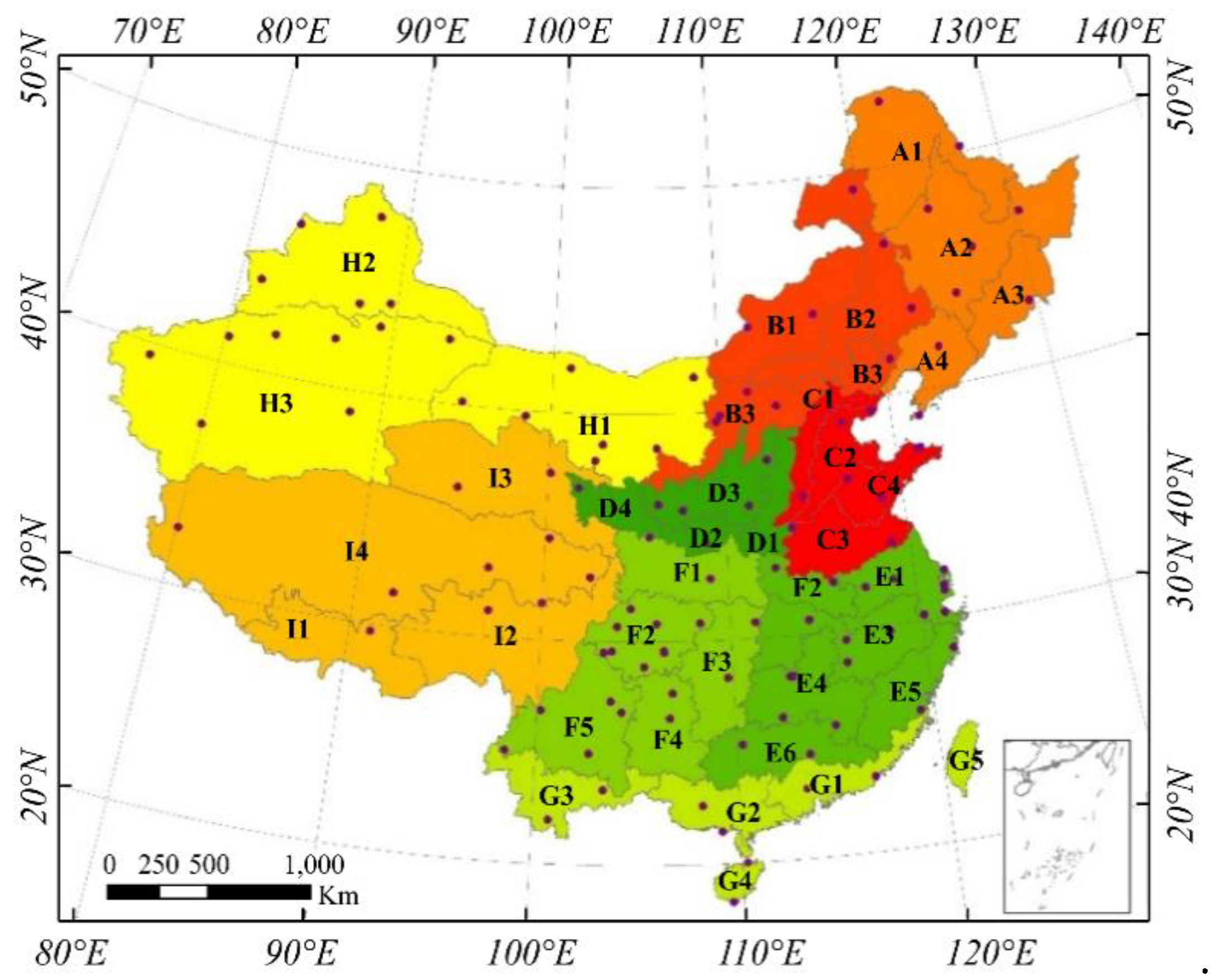
2. Data and Preprocessing

Based on the Ångström–Prescott formula Equation (1) recommended by FAO 56 [5], the data used in this study comprised solar radiation (R_s), relative sunshine duration (n/N), extraterrestrial radiation (R_a), and Chinese agricultural comprehensive zone data. R_s uses the monthly total solar radiation from the Dataset of Monthly Values of Radiation Data from Chinese Surface Stations and n/N uses the monthly average daily relative sunshine duration from the Dataset of Monthly Values of Climate Data from Chinese Surface Stations, both datasets are released by the China Meteorological Data Service Center (CMDC) (http://data.cma.cn/), and all effective observation records are from 1957 to 2015. R_a was the monthly average daily value of each station obtained by longitude and latitude from the Dataset of Monthly Values of Climate Data and according to the calculation procedures for daily extraterrestrial radiation suggested in FAO 56. The Chinese agricultural zones data are from China’s comprehensive agricultural zone map (Figure 1) released by the country’s national agricultural committee.

$${\mathrm{R}}_{\mathrm{s}}=\left({\mathrm{a}}_{\mathrm{s}}{+\mathrm{b}}_{\mathrm{s}}\frac{\mathrm{n}}{\mathrm{N}}\right){\mathrm{R}}_{\mathrm{a}}$$

(1)

where R_s is solar radiation (MJm⁻²day⁻¹); n is the actual duration of sunshine (h); N is the maximum possible duration of sunshine or daylight (h); n/N is relative sunshine duration or sunshine percentage; R_a is extraterrestrial radiation (MJm^Ȓ2day⁻¹); a_s is a regression constant expressing the fraction of extraterrestrial radiation reaching Earth on overcast days (n = 0); and a_s + b_s is the fraction of extraterrestrial radiation reaching the earth on clear days (n = N).

2.1. Data Preprocessing

The first step was to unify the time scale unit. The total monthly solar radiation data were converted into the average daily value, and matched one to one with the n/N data by station number. The data from 124 stations were obtained (Figure 1). Simultaneously, the latitude and longitude of the stations were extracted from the metadata of the Dataset of Monthly Values of Climate Data from Chinese Surface Stations. On the one hand, the R_a could be calculated by using it; on the other hand, it could be spatialized (Figure 1) by GIS software such as ArcGIS.

The second step was to perform quality filtering. Theoretically, the R_s of ground observations are definitely lower than R_a, owing to the presence of atmospheric interference. However, in actual observations, there is an anomaly in which R_s is greater than R_a in the observation results due to instrument damage or human error. Therefore, outliers should be removed.

The third step was to find the zonal statistics of the station data using vector data of the agricultural comprehensive zones obtained after spatial adjustment to avoid the discontinuity of the time series of the station data. The station average value of the effective observed data in an agricultural sub-zone was used to represent the observation value of this sub-zone. Subsequently, the agricultural sub-zone was used as the basic spatial unit in the calculation. The continuous effective data of all agricultural zones from 1961 to 2015 were finally obtained.

2.2. Technical Program

The main process used in this study to calibrate the Ångström–Prescott parameters consists of four parts: data grouping, calculating the coefficients a_s and b_s based on the corrected data of different time scales, determining the best corrected data time scale for calculating a_s and b_s, and determining the optimal a_s and b_s coefficients. A flowchart of the specific steps taken to correct the parameters of the Ångström–Prescott formula is shown in Figure 2.

(1)

Table 1. Data grouping.

Group ID	Group 1	Group 2	Group 3	Group 4	Group 5	Group 6	Group 7	Time Scale
Validation data set	2011–2015	2006–2010	2001–2005	1996–2000	1991–1995	1986–1990	1981–1985	5 y
Correction data set	2010–2006	2005–2001	2000–1996	1995–1991	1990–1986	1985–1981	1980–1976	5 y
	2010–2001	2005–1996	2000–1991	1995–1986	1990–1981	1985–1976	1980–1971	10 y
	2010–1996	2005–1991	2000–1986	1995–1981	1990–1976	1985–1971	1980–1966	15 y
	2010–1991	2005–1986	2000–1981	1995–1976	1990–1971	1985–1966	1980–1961	20 y
	2010–1986	2005–1981	2000–1976	1995–1971	1990–1966	1985–1961		25 y
	2010–1981	2005–1976	2000–1971	1995–1966	1990–1961			30 y
	2010–1976	2005–1971	2000–1966	1995–1961				35 y
	2010–1971	2005–1966	2000–1961					40 y
	2010–1966	2005–1961						45 y
	2010–1961							50 y

provides details on how the data were grouped. The data from 1961 to 2015 were divided into a correction data set and a validation data set. The validation data set comprised seven groups of five-year intervals: 2011–2015, 2006–2010, 2001–2006, 1996–2000, 1991–1995, 1986–1990, and 1981–1985. This means the validation data were fixed for each group. The correction data set was also divided into seven groups corresponding to the former: 2010–1961, 2005–1961, 2000–1961, 1995–1961, 1990–1961, 1985–1961, and 1980–1961. To determine the precision of a_s and b_s from the corrected data at different time scales, the corrected data were further divided into 5 years, 10 years, 15 years and other corrected data time scales by reverse order in steps of five years.

(2) Coefficients a_s and b_s were calculated based on different time scale corrected data. First, the monthly average multi-year values of the different data scales in different groups were obtained. That is the n/N, R_s, and R_a of each agricultural area were obtained for January to December at specific corrected data time scales. There were three groups of data, with 12 values in each group. Secondly, R_s/R_a was taken as the dependent variable and n/N as the independent variable. The unified coefficients a_s and b_s of each agricultural area within a year were then calculated based on the least squares regression method. In the regression process, the constraint calculation was carried out according to Equation (2).

$$\{\begin{array}{l}0<{\mathrm{a}}_s<1\\ 0<b_s<1\\ 0<{\mathrm{a}}_s+b_s<1\end{array}$$

(2)

(3) The best corrected data time scales for calculating coefficients a_s and b_s were determined. The estimation value of solar radiation (R_{s_c}) was calculated monthly using the a_s and b_s coefficients from the above step in the validation data. Then, based on the relative error index algorithm, which is simple and can be easily interpreted by ordinary users, the five-year average relative error of R_{s_c} was calculated with the corresponding true R_s value (from observation). By analyzing the change ranges in the average relative error in all areas, the range of the averages of monthly regional error within a year and the frequency of the corrected data time scale corresponding to the minimum of monthly regional error, the best corrected data time scale for calibrating the a_s and b_s coefficients was obtained.

(4) The optimal a_s and b_s coefficients were determined using the following steps. First, the a_s and b_s coefficients recommended in the current research and application were selected. Again, based on relative error, the relative accuracy of monthly R_{s_c} calculated using this figure and the FAO’s recommended values were compared. Finally, the a_s and b_s values corresponding to the R_{s_c} with the highest accuracy were selected as the optimal coefficients.

3. Results and Analysis

3.1. Optimum Best Corrected Data Time Scale

Table 2. Relative error range of R_{s_c} calculated based on the recommended Food and Agriculture Organization of the United Nations (FAO) value and coefficients a_s and b_s of each time scale corrected data in China.

Group ID.	Group 1	Group 2	Group 3	Group 4	Group 5	Group 6	Group 7	Time Scale
Validation data set	2011–2015	2006–2010	2001–2005	1996–2000	1991–1995	1986–1990	1981–1985	5 y
Relative error range of Rs_c from as and bs recommended by FAO	1–62%	1–60%	1–61%	1–70%	1–85%	1–93%	1–84%	5 y
Relative error range of Rs_c from as and bs by correction data set	1–22%	1–19%	1–23%	1–30%	1–27%	1–34%	1–30%	5 y
	1–24%	1–25%	1–25%	1–30%	1–28%	1–34%	1–32%	10 y
	1–24%	1–28%	1–21%	1–24%	1–28%	1–33%	1–37%	15 y
	1–25%	1–28%	1–24%	1–24%	1–28%	1–34%	1–39%	20 y
	1–26%	1–25%	1–21%	1–25%	1–28%	1–34%		25 y
	1–26%	1–24%	1–22%	1–24%	1–30%			30 y
	1–26%	1–24%	1–22%	1–24%				35 y
	1–26%	1–24%	1–25%					40 y
	1–26%	1–23%						45 y
	1–26%							50 y

shows the range of variation of the national five-year average relative error of R_{s_c} within a year, which was calculated using the a_s and b_s coefficients suggested by FAO and the corrected values obtained under different corrected data time scales in each group. It shows that in both the R_{s_c} calculated based on the a_s and b_s coefficients from FAO and that from the corrected data, there is an at least 1% average relative error. However, the range of the relative error (maximum - minimum) based on the former is higher than that obtained by the latter. This illustrates the necessity of calibrating the a_s and b_s coefficients for the local data.

There was no significant difference in the range of the relative error of R_{s_c} calculated based on the a_s and b_s coefficients from different time scale corrected data in each group. The corresponding error range of 5–20 years fluctuated slightly. Further, the corresponding error range after 20 years has basically been stable; apart from group 4 and 2, the range of the other groups tended to increase slightly. Therefore, from the perspective of the range in variation of the relative error, the optimal corrected data time scale for the regression of the a_s and b_s coefficients within a year is at most 20 years. The corrected data of longer time series have little effect on reducing the range of the relative error. Further selection of the best corrected data time scale needs to compare other statistical indicators of the calibration results within 20 years.

Table 3. Range of R_{s_c} monthly average relative error in China.

Group ID	Group 1	Group 2	Group 3	Group 4	Group 5	Group 6	Group 7	Time Scale
Validation data set	2011–2015	2006–2010	2001–2005	1996–2000	1991–1995	1986–1990	1981–1985	5 y
Range value of relative error	2%	1%	2%	3%	1%	2%	2%	5 y
	2%	1%	2%	2%	2%	2%	3%	10 y
	2%	1%	2%	2%	1%	2%	2%	15 y
	2%	2%	1%	2%	2%	3%	3%	20 y

is the range value of the monthly national average relative error of R_{s_c} within a year, which was calculated based on the a_s and b_s coefficients obtained from the corrected data from each group of 5–20 years. The table shows that the variation of relative error within the year obtained from the 5–20 year scale corrected data for each group is not obvious and most of them are within 2%. Comparatively speaking, this frequency is slightly higher on 10-year and 15-year scales than on a 5-year and 20-year scales; thus, the results of the former are relatively stable.

Further comparisons of the monthly national average of the relative error of R_{s_c} for the 10- and 15-year scales corrected data in each group shows (Figure 3) that, for 10 of 12 months within a year, there are more than 50% of the groups with average relative error of R_{s_c} from the former lower than that from the later. Furthermore, in 12 months, the cumulative frequency of the 10-year data scale corresponding to the minimum national average relative error is > 60%.

Therefore, this study determined that 10 years is the best corrected data time scale for calibrating the a_s and b_s coefficients.

3.2. Optimizing Coefficients a_s and b_s

In terms of the current research applications, this study recommends directly selecting the a_s and b_s coefficients calculated from the corrected data from 2010 to 2001. However, when it comes to the monthly application in each agricultural zone, a comparison of the R_{s_c} accuracy in the 2011 to 2015 data value shows that differences exist within a year for each zone. Figure 4 presents the results of a comparison of the R_{s_c} relative error from the a_s and b_s coefficients corrected based on data from 2010 to 2001 and the FAO recommended value within a year by zone. The numbers in red font indicate that the R_{s_c} calculated from the a_s and b_s coefficient corrected results are better than those recommended by the FAO; this means that the R_{s_c} relative error from the a_s and b_s coefficients corrected based on data from 2010 to 2001 is lower than the R_{s_c} relative error from the a_s and b_s coefficients recommended by the FAO. The numbers in black font indicate that the R_{s_c} calculated from the FAO recommended a_s and b_s coefficients is superior to the calibration results; this means that the R_{s_c} relative error from the a_s and b_s coefficients recommended by the FAO is lower than the R_{s_c} relative error from the a_s and b_s coefficient corrected based on data from 2010 to 2001. The number “0” signifies that the absolute difference of two relative errors is greater than zero and less than 50%, and the number “1” signifies that the absolute difference of two relative errors is equal to or greater than 50% and less than 150%. For red numbers, the larger the value, the greater the improvement in the accuracy of R_{s_c} after calibration. For black numbers, the opposite is true. In more than two-thirds of the agricultural zones, there are varying degrees that the FAO recommended value is better than the correction value within a year; this is most obvious in areas A and B.

Because the corrected a_s and b_s coefficients are not reliable in the verification results for agricultural zones within a year, it is considered that a combination of the correction values of the a_s and b_s coefficients and the FAO recommended values is the best scheme for practical research and application. Thus, based on the comparison results (Figure 4) of the relative error of R_{s_c} estimated from the corrected a_s and b_s coefficients and the FAO recommended values by zone and month, the smaller the relative error R_{s_c} calculated using the correction coefficients and the FAO’s recommended values, the closer the corresponding value is to R_{s_o}; therefore, the a_s and b_s values with the lower R_{s_c} relative error are retained as the optimization parameters (

Table 4. Best parameters of the Ångström–Prescott formula in agricultural zones of China.

Region ID	January		February		March		April		May		June		July		August		September		October		November		December
	as	bs	as	bs	as	bs	as	bs	as	bs	as	bs	as	bs	as	bs	as	bs	as	bs	as	bs	as	bs
A1	0.25	0.50	0.14	0.65	0.25	0.50	0.25	0.50	0.25	0.50	0.25	0.50	0.25	0.50	0.25	0.50	0.25	0.50	0.25	0.50	0.25	0.50	0.25	0.50
A2	0.25	0.50	0.25	0.50	0.19	0.58	0.19	0.58	0.25	0.50	0.19	0.58	0.25	0.50	0.25	0.50	0.25	0.50	0.25	0.50	0.25	0.50	0.25	0.50
A3	0.25	0.50	0.25	0.50	0.25	0.50	0.25	0.50	0.25	0.50	0.25	0.50	0.25	0.50	0.25	0.50	0.19	0.56	0.19	0.56	0.25	0.50	0.25	0.50
A4	0.17	0.58	0.17	0.58	0.17	0.58	0.17	0.58	0.17	0.58	0.17	0.58	0.17	0.58	0.17	0.58	0.17	0.58	0.17	0.58	0.17	0.58	0.17	0.58
B1	0.25	0.50	0.25	0.50	0.25	0.50	0.25	0.50	0.25	0.50	0.25	0.50	0.25	0.50	0.25	0.50	0.25	0.50	0.25	0.50	0.25	0.50	0.25	0.50
B2	0.25	0.50	0.25	0.50	0.25	0.50	0.25	0.50	0.25	0.50	0.24	0.46	0.24	0.46	0.25	0.50	0.24	0.46	0.25	0.50	0.25	0.50	0.25	0.50
B3	0.22	0.49	0.22	0.49	0.25	0.50	0.25	0.50	0.25	0.50	0.25	0.50	0.25	0.50	0.25	0.50	0.22	0.49	0.25	0.50	0.22	0.49	0.25	0.50
C1	0.27	0.34	0.25	0.50	0.25	0.50	0.25	0.50	0.25	0.50	0.27	0.34	0.27	0.34	0.25	0.50	0.27	0.34	0.25	0.50	0.27	0.34	0.27	0.34
C2	0.22	0.49	0.22	0.49	0.22	0.49	0.22	0.49	0.22	0.49	0.22	0.49	0.22	0.49	0.22	0.49	0.22	0.49	0.22	0.49	0.22	0.49	0.22	0.49
C3	0.22	0.47	0.22	0.47	0.25	0.50	0.25	0.50	0.22	0.47	0.22	0.47	0.22	0.47	0.22	0.47	0.25	0.50	0.22	0.47	0.22	0.47	0.22	0.47
C4	0.20	0.51	0.20	0.51	0.20	0.51	0.20	0.51	0.20	0.51	0.20	0.51	0.20	0.51	0.20	0.51	0.20	0.51	0.20	0.51	0.20	0.51	0.20	0.51
D1	0.26	0.32	0.26	0.32	0.26	0.32	0.25	0.50	0.25	0.50	0.26	0.32	0.25	0.50	0.26	0.32	0.26	0.32	0.26	0.32	0.26	0.32	0.26	0.32
D2	0.21	0.44	0.21	0.44	0.21	0.44	0.21	0.44	0.21	0.44	0.21	0.44	0.21	0.44	0.21	0.44	0.21	0.44	0.21	0.44	0.21	0.44	0.21	0.44
D3	0.17	0.55	0.25	0.50	0.25	0.50	0.25	0.50	0.25	0.50	0.17	0.55	0.17	0.55	0.17	0.55	0.17	0.55	0.17	0.55	0.17	0.55	0.17	0.55
D4	0.25	0.50	0.25	0.50	0.25	0.50	0.21	0.54	0.21	0.54	0.21	0.54	0.21	0.54	0.21	0.54	0.21	0.54	0.25	0.50	0.25	0.50	0.25	0.50
E1	0.15	0.59	0.15	0.59	0.15	0.59	0.15	0.59	0.15	0.59	0.15	0.59	0.15	0.59	0.15	0.59	0.15	0.59	0.15	0.59	0.15	0.59	0.15	0.59
E2	0.25	0.50	0.25	0.50	0.19	0.49	0.19	0.49	0.19	0.49	0.19	0.49	0.19	0.49	0.19	0.49	0.19	0.49	0.25	0.50	0.19	0.49	0.19	0.49
E3	0.10	0.67	0.10	0.67	0.10	0.67	0.10	0.67	0.10	0.67	0.10	0.67	0.10	0.67	0.10	0.67	0.10	0.67	0.10	0.67	0.10	0.67	0.10	0.67
E4	0.10	0.67	0.10	0.67	0.10	0.67	0.10	0.67	0.10	0.67	0.10	0.67	0.10	0.67	0.10	0.67	0.10	0.67	0.10	0.67	0.10	0.67	0.10	0.67
E5	0.15	0.62	0.15	0.62	0.15	0.62	0.15	0.62	0.15	0.62	0.15	0.62	0.15	0.62	0.15	0.62	0.15	0.62	0.15	0.62	0.15	0.62	0.15	0.62
E6	0.13	0.66	0.13	0.66	0.13	0.66	0.13	0.66	0.13	0.66	0.25	0.50	0.13	0.66	0.13	0.66	0.25	0.50	0.25	0.50	0.13	0.66	0.13	0.66
F1	0.16	0.51	0.16	0.51	0.16	0.51	0.16	0.51	0.16	0.51	0.16	0.51	0.25	0.50	0.16	0.51	0.16	0.51	0.16	0.51	0.16	0.51	0.16	0.51
F2	0.16	0.65	0.16	0.65	0.16	0.65	0.16	0.65	0.16	0.65	0.16	0.65	0.16	0.65	0.16	0.65	0.16	0.65	0.16	0.65	0.16	0.65	0.16	0.65
F3	0.13	0.70	0.13	0.70	0.13	0.70	0.13	0.70	0.13	0.70	0.13	0.70	0.13	0.70	0.13	0.70	0.13	0.70	0.13	0.70	0.13	0.70	0.13	0.70
F4	0.14	0.83	0.14	0.83	0.25	0.50	0.14	0.83	0.25	0.50	0.25	0.50	0.25	0.50	0.14	0.83	0.14	0.83	0.25	0.50	0.25	0.50	0.14	0.83
F5	0.23	0.49	0.23	0.49	0.23	0.49	0.23	0.49	0.23	0.49	0.23	0.49	0.23	0.49	0.23	0.49	0.23	0.49	0.23	0.49	0.25	0.50	0.23	0.49
G1	0.25	0.50	0.16	0.56	0.16	0.56	0.16	0.56	0.16	0.56	0.16	0.56	0.16	0.56	0.16	0.56	0.16	0.56	0.25	0.50	0.25	0.50	0.25	0.50
G2	0.16	0.63	0.16	0.63	0.16	0.63	0.16	0.63	0.16	0.63	0.16	0.63	0.16	0.63	0.16	0.63	0.16	0.63	0.16	0.63	0.25	0.50	0.16	0.63
G3	0.25	0.50	0.25	0.50	0.29	0.37	0.29	0.37	0.29	0.37	0.29	0.37	0.29	0.37	0.29	0.37	0.25	0.50	0.25	0.50	0.29	0.37	0.29	0.37
G4	0.25	0.50	0.33	0.29	0.25	0.50	0.25	0.50	0.25	0.50	0.25	0.50	0.25	0.50	0.25	0.50	0.25	0.50	0.25	0.50	0.25	0.50	0.25	0.50
H1	0.25	0.50	0.25	0.49	0.25	0.50	0.25	0.50	0.25	0.50	0.25	0.49	0.25	0.49	0.25	0.49	0.25	0.49	0.25	0.50	0.25	0.49	0.25	0.49
H2	0.25	0.50	0.27	0.44	0.25	0.50	0.27	0.44	0.27	0.44	0.27	0.44	0.27	0.44	0.27	0.44	0.25	0.50	0.27	0.44	0.27	0.44	0.27	0.44
H3	0.21	0.51	0.21	0.51	0.21	0.51	0.21	0.51	0.21	0.51	0.25	0.50	0.25	0.50	0.21	0.51	0.21	0.51	0.21	0.51	0.21	0.51	0.21	0.51
I1	0.25	0.60	0.25	0.60	0.25	0.60	0.25	0.50	0.25	0.60	0.25	0.60	0.25	0.60	0.25	0.60	0.25	0.60	0.25	0.60	0.25	0.60	0.25	0.60
I2	0.25	0.56	0.25	0.56	0.25	0.56	0.25	0.56	0.25	0.50	0.25	0.56	0.25	0.56	0.25	0.56	0.25	0.56	0.25	0.56	0.25	0.56	0.25	0.56
I3	0.24	0.57	0.24	0.57	0.24	0.57	0.24	0.57	0.24	0.57	0.24	0.57	0.24	0.57	0.24	0.57	0.24	0.57	0.24	0.57	0.24	0.57	0.24	0.57
I4	0.20	0.67	0.20	0.67	0.20	0.67	0.20	0.67	0.20	0.67	0.20	0.67	0.20	0.67	0.20	0.67	0.20	0.67	0.20	0.67	0.20	0.67	0.20	0.67

).

4. Discussion

4.1. Influence of Data Processing Mode On the Research Results

After data preprocessing, 124 stations were selected; however, all stations were established at different times. During the observation period, some stations were relocated, some instruments were damaged, and some observation tasks were changed, resulting in the time discontinuities in the observation data. To correct this, this study adopted the average processing method for the filtered data from each station. However, this resulted in the following problems. Firstly, the direct average processing method does not consider the influence of other geographical factors, such as terrain, which may cause systematic errors. Secondly, the spatial distribution of meteorological stations is not uniform (Figure 1). Station density is also inconsistent in the 38 agricultural sub-zones, and there is a difference in the sample size between regions. Zones with few stations may be under-represented. In addition, if a station value is missing in a certain period, it may cause the average value of the station in this period to become unrepresentative. Finally, to obtain the unified values of the a_s and b_s coefficients within a year, there were only 12 data points for each element in each zone for the regression; this ignores the seasonal changes in the atmospheric state under typical monsoon climate conditions in China.

4.2. Random Errors and Data Quality Problems

According to Equation (1), using a simple least-squares regression (non-parameter constraint) to get the a_s and b_s coefficients should, in theory, accord with the constraint conditions presented in Equation (2). However, the regression results were found, directly using the non-parameter constraint for seven groups in this study, that did not meet the constraint condition; this means that the FAO suggestion value needs to be set as the initial value to further constrain the regression. One possible reason for this is that the n/N and R_s observation values still have errors after the initial quality control. In addition, the verified R_{s_c} results, calculated using the corrected a_s and b_s coefficients, are all based on the average value of the five-year verified data. If the results are decomposed into various verification years, they may be affected by the random errors between the years, and the rules in the variations of the errors between years may not be obvious. Finally, outliers conforming to the quality control rules cannot be identified in the data processing process. Furthermore, with the development of modern meteorological observation technology, there is a difference in the quality of the observed data from different stages, which may also be a source of the “anomalies” in the above results.

4.3. Optimization of Coefficients a_s and b_s in Practice

This study determined that, for current research and applications, the calibrated values of coefficients a_s and b_s based on data from 2010 to 2001 should be selected as the recommended parameters for the Ångström–Prescott formula. The average relative error of R_{s_c} from 2011 to 2015 calculated using this formula and the FAO recommended value were compared to select the best parameter values (Table 4). However, if the optimal values of the a_s and b_s coefficients were selected by comparing the average relative errors of longer or shorter time series or the relative errors of a single year, the results would likely change. Thus, based on the existing data, the next step would be to introduce a new algorithm to solve these problems and further improve the estimation accuracy of R_s. In addition, the period of the verification data between groups in this study is not consistent and the a_s and b_s coefficients obtained from the same time scale data of between groups differ. Therefore, the inter-annual variation of the a_s and b_s coefficients and the variation of R_{s_c} precision with time in their applications also need to be studied and discussed further.

5. Conclusions

This study referenced China’s division of the nine main types of agricultural land into 38 agricultural zones and used these as a study area. Coefficients a_s and b_s were investigated and corrected by zone at different corrected data time scales based on the average daily value of the meteorological data, as recorded in the Dataset of Monthly Values of Radiation Data from Chinese Surface Stations and the Dataset of Monthly Values of Climate Data from Chinese Surface Stations. The data were taken for 124 stations from 1957 to 2015. Using the least-squares regression method, this study analyzed the influence of different time scales corrected data on the accuracy thereof and determined the optimum correction coefficients of 38 agricultural sub-zones. The main conclusions are as follows:

(1) The relative error of R_{s_c} calculated by the a_s and b_s coefficients proposed by FAO has a large variation range, which is not completely applicable to China. Compared with the corrected a_s and b_s coefficients, the relative error range of the R_{s_c} calculated is significantly reduced.

(2) 10 years is the best corrected data scale with which to correct the a_s and b_s coefficients. There was no significant difference in the relative error range of R_{s_c} calculated by the a_s and b_s coefficients based on the grouped data at different corrected data time scales. After 20 years, the relative error range of R_{s_c} tended to stabilize and increase slightly. The national average annual range of the R_{s_c} within a year corresponding to the 10-year and 15-year scales is generally slightly more stable than five years and 20 years. When the average relative error of R_{s_c} corresponding to the scale of 10-year and 15-year correction data were further compared, it was found that the national average R_{s_c} relative error corresponding to the 10-year scale in the cumulative period of 60% was lower than the 15-year correction scale when each group was considered on a month by month basis.

(3) By comparing the R_{s_c} relative error, the corrected values of the a_s and b_s coefficients and the FAO suggested values were optimized in different agricultural sub-zones in different months under the existing basic data conditions.

References

1. Djaman, K.; Irmak, S.; Kabenge, I.; Futakuchi, K. Evaluation of FAO-56 Penman-Monteith Model with Limited Data and the Valiantzas Models for Estimating Grass-Reference Evapotranspiration in Sahelian Conditions. J. Irrig. Drain. Eng. 2016, 142, 04016044. [Google Scholar] [CrossRef]
2. Xu, J.; Peng, S.; Zhang, X.; Ding, J. Applicability of FAO56 and ASCE Penman-Monteith equations for reference crop evapotranspiration calculation on turf grass. Trans. Chin. Soc. Agric. Eng. 2009, 25, 32–37. [Google Scholar]
3. Shunjun, H.; Pan, Y.; Kang, S.; Song, Y.; Tian, C. Comparison of the reference crop evapotranspiration estimated by the Penman-Monteith and Penman methods in Tarim River Basin. Trans. Chin. Soc. Agric. Eng. 2005, 21, 30–35. [Google Scholar]
4. Shizhang, P.; Junzeng, X.; Jiali, D. Influence of as and bs values on determination of reference crop evapotranspiration by Penman-Monteith formula. J. Irrig. Drain. 2006, 25, 5–8. [Google Scholar]
5. Allen, R.G.; Pereira, L.S.; Raes, D.; Smith, M. Crop Evapotranspiration-Guidelines for Computing Crop Water Requirements-FAO Irrigation and Drainage Paper 56; FAO: Rome, Italy, 1998; Volume 300, p. D05109. [Google Scholar]
6. Yao, N.; Li, Y.; Sun, C. Effects of changing climate on reference crop evapotranspiration over 1961–2013 in Xinjiang, China. Theor. Appl. Clim. 2018, 131, 349–362. [Google Scholar] [CrossRef]
7. Liu, X.; Xu, C.; Zhong, X.; Li, Y.; Yuan, X.; Cao, J. Comparison of 16 models for reference crop evapotranspiration against weighing lysimeter measurement. Agric. Water Manag. 2017, 184, 145–155. [Google Scholar] [CrossRef]
8. Li, Y.; Lyu, M.; Zhang, H.; Deng, Z.; Liu, C.; Jiang, M. Sensitivity Analysis of the Reference Crop Evapotranspiration to Meteorological Factors. J. Irrig. Drain. Eng. 2017, 36, 94–99. [Google Scholar]
9. Amri, R.; Zribi, M.; Lili-Chabaane, Z.; Szczypta, C.; Calvet, J.C.; Boulet, G. Using the dual approach of FAO-56 combined with multi-sensor remote sensing for estimating the regional evapotranspiration. In Proceedings of the 2014 1st International Conference on Advanced Technologies for Signal and Image Processing (ATSIP), Sousse, Tunisia, 17–19 March 2014; pp. 373–378. [Google Scholar]
10. Peng, L.; Li, Y.; Feng, H. The best alternative for estimating reference crop evapotranspiration in different sub-regions of mainland China. Sci. Rep. 2017, 7, 1–19. [Google Scholar] [CrossRef] [Green Version]
11. Yan, K.; Wang, Y.; Xu, P.; Fu, B.; Li, C. Adaptation of Hargreaves Methods and Prediction of Reference Crop Evapotranspiration in Minjiang River Headwater Region. Trans. Chin. Soc. Agric. Mach. 2018, 49, 273–281. [Google Scholar]
12. Irmak, S.; Irmak, A.; Jones, J.; Howell, T.A.; Jacobs, J.M.; Allen, R.G.; Hoogenboom, G. Predicting daily net radiation using minimum climatological data. J. Irrig. Drain. Eng. 2003, 129, 256–269. [Google Scholar] [CrossRef]
13. Nandagiri, L.; Kovoor, G.M. Sensitivity of the Food and Agriculture Organization Penman–Monteith evapotranspiration estimates to alternative procedures for estimation of parameters. J. Irrig. Drain. Eng. 2005, 131, 238–248. [Google Scholar] [CrossRef]
14. Yoder, R.E.; Odhiambo, L.O.; Wright, W.C. Effects of vapor-pressure deficit and net-irradiance calculation methods on accuracy of standardized Penman-Monteith equation in a humid climate. J. Irrig. Drain. Eng. 2005, 131, 228–237. [Google Scholar] [CrossRef]
15. Ju, X.; Tu, Q.; Li, Q. Discussion on the climatological calculation of solar radiation. J. Nanjing Inst. Meteorol. 2005, 28, 516–521. [Google Scholar]
16. Yang, G.; Wang, Z.; Wang, H.; Jia, Y. Potential evapotranspiration evolution rule and its sensitivity analysis in Haihe River basin. Adv. Water Sci. 2009, 20, 409–415. [Google Scholar]
17. Tamm, T. Effect of Meteorological Conditions and Water Management on Hydrological Processes in Agricultural Fields: Parameterization and Modeling of Estonian Case Studies. Master’s Thesis, Helsinki University of Technology, Helsinki, Finland, 2002. [Google Scholar]
18. Kjærsgaard, J.H.; Plauborg, F.; Hansen, S. Comparison of models for calculating daytime long-wave irradiance using long term data set. Agric. For. Meteor. 2007, 143, 49–63. [Google Scholar] [CrossRef]
19. Lu, Y.; Hong, T.; Lu, J.; Wen, H. Spatial-temporal variation characteristics of gross solar radiation in Anhui Province from 1961 to 2010. Meteor. Sci. Tech. 2016, 44, 769–775. [Google Scholar]
20. Cui, R.X. The analysis of spatiotemporal variation characteristics of global solar radiation in Shandong Province. J. Nat. Res. 2014, 29, 1780–1791. [Google Scholar]
21. Zhao, J.; Li, W.P.; Li, F. Climatological calculation and analysis of global solar radiation in the Loess Plateau. Arid Zone Res. 2008, 25, 53–58. [Google Scholar] [CrossRef]
22. Du, D.; Mao, H.; Liu, A.; Pan, W. The climatological calculation and distributive character of global solar radiation in Guangdong province. Resour. Sci. 2003, 25, 66–70. [Google Scholar]
23. Miao, M.; Yan, H.; Yan, Z. The distribution characteristics of total solar radiation in Jiangsu Province. J. Meteorol. Sci. 2012, 32, 269–274. [Google Scholar]
24. Ma, J.; Luo, Y.; Shen, Y.; Liang, S.; Li, H. Regional long-term trend of ground solar radiation in China over the past 50 years. Sci. China Earth Sci. 2013, 56, 1242–1253. [Google Scholar] [CrossRef]
25. Yin, Y.; Wu, S.; Zheng, D.; Yang, Q. Radiation calibration of FAO56 Penman–Monteith model to estimate reference crop evapotranspiration in China. Agric. Water Manag. 2008, 95, 77–84. [Google Scholar] [CrossRef]
26. Hu, Q.F.; Yang, D.W.; Wang, Y.T.; Yang, H. Effects of Angstrom coefficients on ET (0) estimation and the applicability of FAO recommended coefficient values in China. Adv. Water Sci. 2010, 21, 644–652. [Google Scholar]
27. Liu, X.; Mei, X.; Li, Y.; Wang, Q.; Zhang, Y.; Porter, J.R. Variation in reference crop evapotranspiration caused by the Ångström–Prescott coefficient: Locally calibrated versus the FAO recommended. Agric. Water Manag. 2009, 96, 1137–1145. [Google Scholar] [CrossRef]
28. Wen, C.; Ying, X.; Chunfeng, D. Research on applicability of solar radiation parametric model in Anhui province. Chin. Agric. Sci. Bull. 2014, 30, 207–212. [Google Scholar]
29. Yuan, H.; Yuan, X.; Tang, G.; Cui, Y.; Jiang, S. Correction of parameters in Angstrom formula and analysis of total solar radiation characteristics in Huaibei plain. J. Drain. Irrig. Mach. Eng. 2018, 36, 426–432. [Google Scholar]
30. Li, M.; Mei, X.; Zhong, X.; Liu, X.; Hao, W.; Han, H.; Liu, W. Parameterization of Ångström-Prescott radiation model in Yunnan province. Trans. Chin. Soc. Agric. Eng. 2012, 28, 100–105. [Google Scholar]
31. Chen, J.L.; He, L.; Wen, Z.F.; Lv, M.Q.; Yi, X.X.; Wu, S.J. A general empirical model for estimation of solar radiation in Yangtze River basin. Appl. Ecol. Environ. Res. 2018, 16, 1471–1482. [Google Scholar] [CrossRef]
32. Liu, X.; Li, Y.; Zhong, X.; Zhao, C.; Jensen, J.R.; Zhao, Y. Towards increasing availability of the Ångström–Prescott radiation parameters across China: Spatial trend and modeling. Energy Convers Manag. 2014, 87, 975–989. [Google Scholar] [CrossRef]
Figure 1. Agricultural comprehensive zone and data station locations. (A. Northeastern China. A1: Khingan, A2: Songnen and Sanjiang plain, A3: Changbai Mountains; A4 Liaoning plain; B. Inner Mongolia and region along the Great Wall. B1: northern Inner Mongolia, B2: central and southern Inner Mongolia, B3: region along the Great Wall; C. Huanghuaihai. C1: piedmont at the foot of the Yanshan and Taihang Mountains, C2: low-lying plain regions of Hebei, Shandong, and Henan, C3: Huang-huai plain, C4: hilly region of Shandong; D. Loess plateau. D1: hilly region of western Henan and eastern Shanxi, D2: Fenhe and Weihe valleys; D3: hilly loess region of Shanxi, Shaanxi, and Gansu, D4: hilly region of central Gansu and eastern Qinghai; E. Middle and lower reaches of the Yangtze River. E1: lower Yangtze plain; E2: mountainous regions of Henan, Hubei, and Anhui, E3: plains in the middle reaches of the Yangtze River, E4: hilly regions south of the Yangtze River; E5: hilly region of Zhejiang and Fujian, E6: hilly regions of Nanling; F. Southwestern China. F1: Qinling and Daba Mountains; F2: Sichuan Basin, F3: border between Sichuan, Hubei, Hunan, and Guizhou, F4: Guizhou and Guangxi plateau, F5: Sichuan and Yunnan plateau; G. Southern China. G1: southern Fujian and central Guangdong, G2: western Guangdong and southern Guangxij, G3: southern Yunnan, G4: Hainan and South China Sea islands; H. Gansu and Xinjiang. H1: border between Inner Mongolia, Ningxia, and Gansu, H2: northern Xinjiang, H3: southern Xinjiang; I. Tibet. I1: southern Tibet, I2: border between Sichuan and Tibet, I3: border between Qinghai and Gansu, I4: high cold region of Tibet.).
Water 11 01706 g001
Figure 2. Process used to correct Ångström–Prescott formula parameters.
Water 11 01706 g002
Figure 3. Corrected data time scale frequency corresponding to the minimum national average relative error of Rs_c in each group.
Water 11 01706 g003
Figure 4. Average relative error comparison results of Rs_c from 2011 to 2015 calculated based on the correction values of coefficients as and bs from 2010 to 2001 data and the FAO recommended value, respectively. (Red font indicates that the Rs_c calculated from the as and bs coefficient correction results are better than those recommended by the FAO, and vice versa.).
Water 11 01706 g004