Inter-Comparison of Different Bayesian Model Averaging Modifications in Streamflow Simulation

Abstract
1. Introduction
2. Materials and Methods
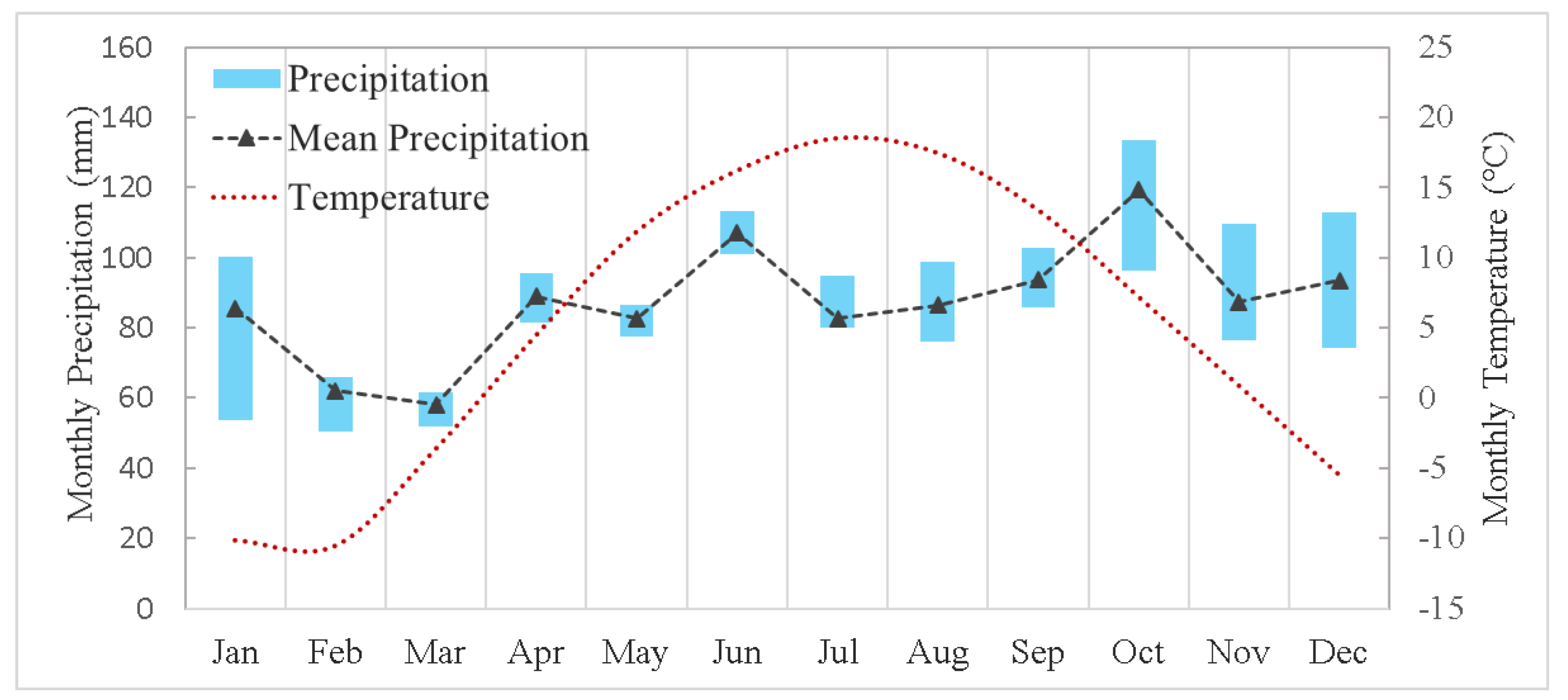
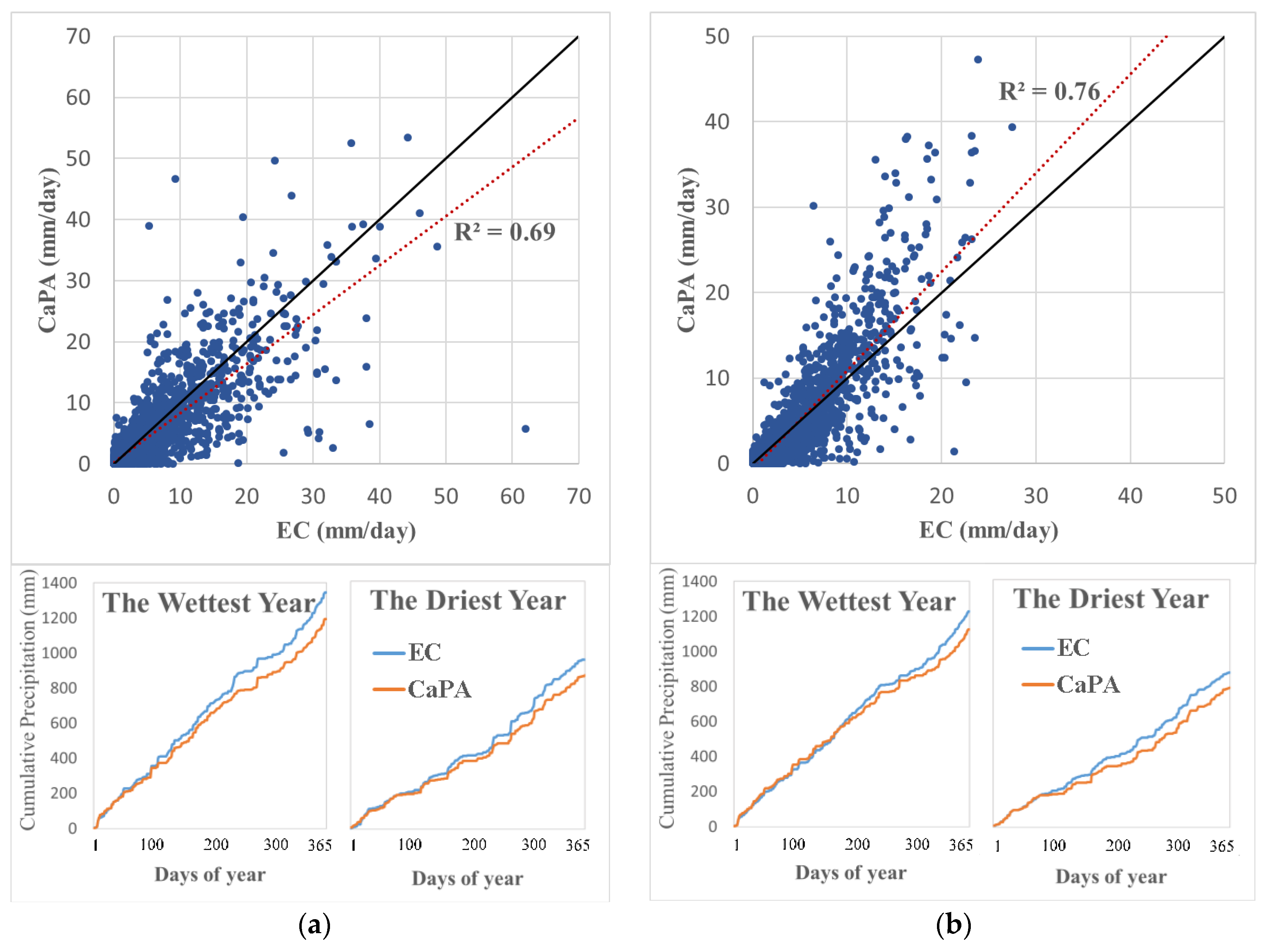
2.1. Study Area and Data
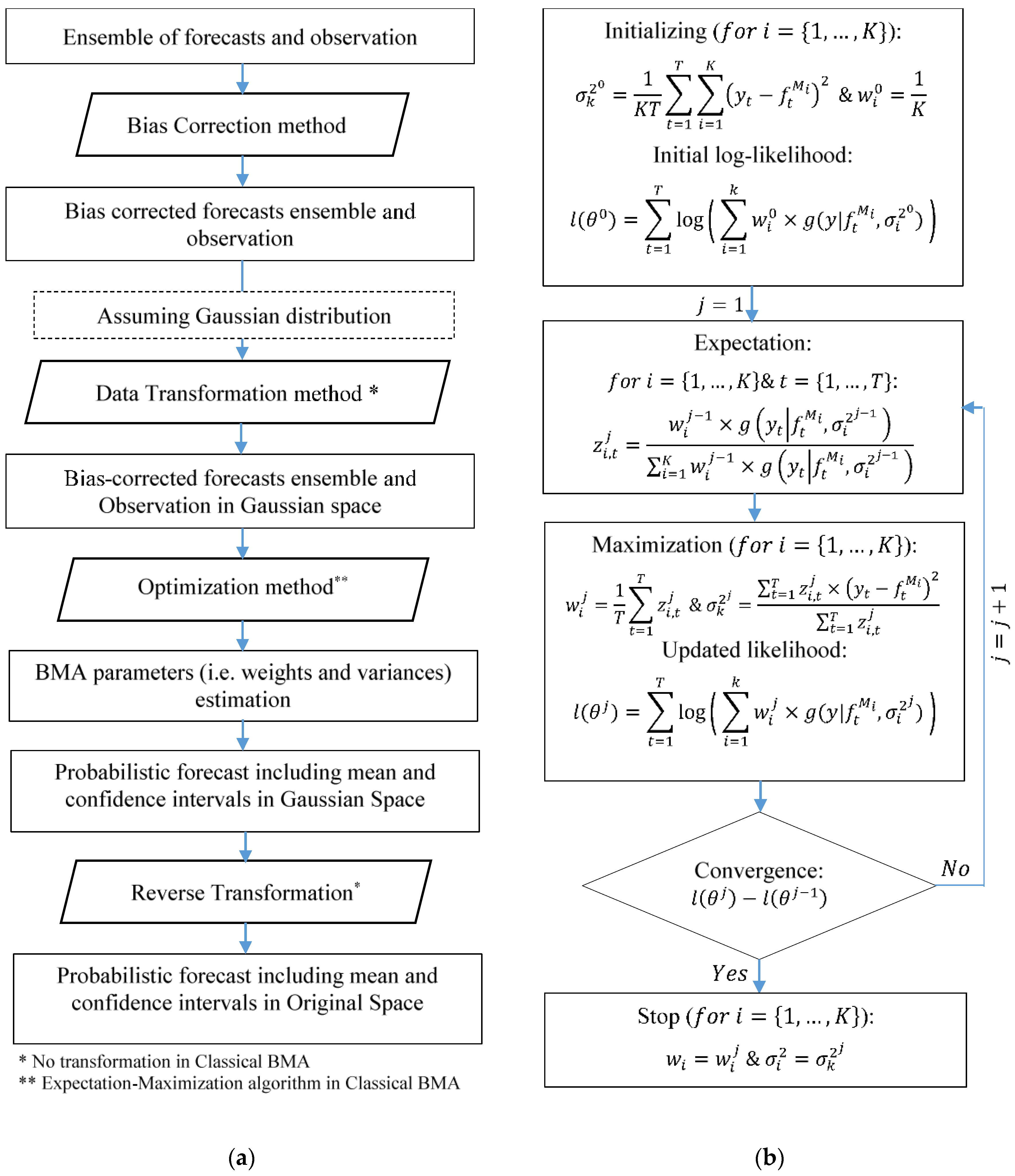
2.2. Standard Bayesian Model Averaging Technique
2.3. BMA Scenario-Based Analysis
2.3.1. Streamflow Ensemble
2.3.2. Data Transformation Methods
2.3.3. Distribution Types
2.3.4. Standard Deviation Types
2.3.5. Optimization Methods
2.4. Hydrological Models
2.5. Performance Evaluation Metrics
3. Results and Discussion
3.1. Choosing the Best Ensemble Scenario
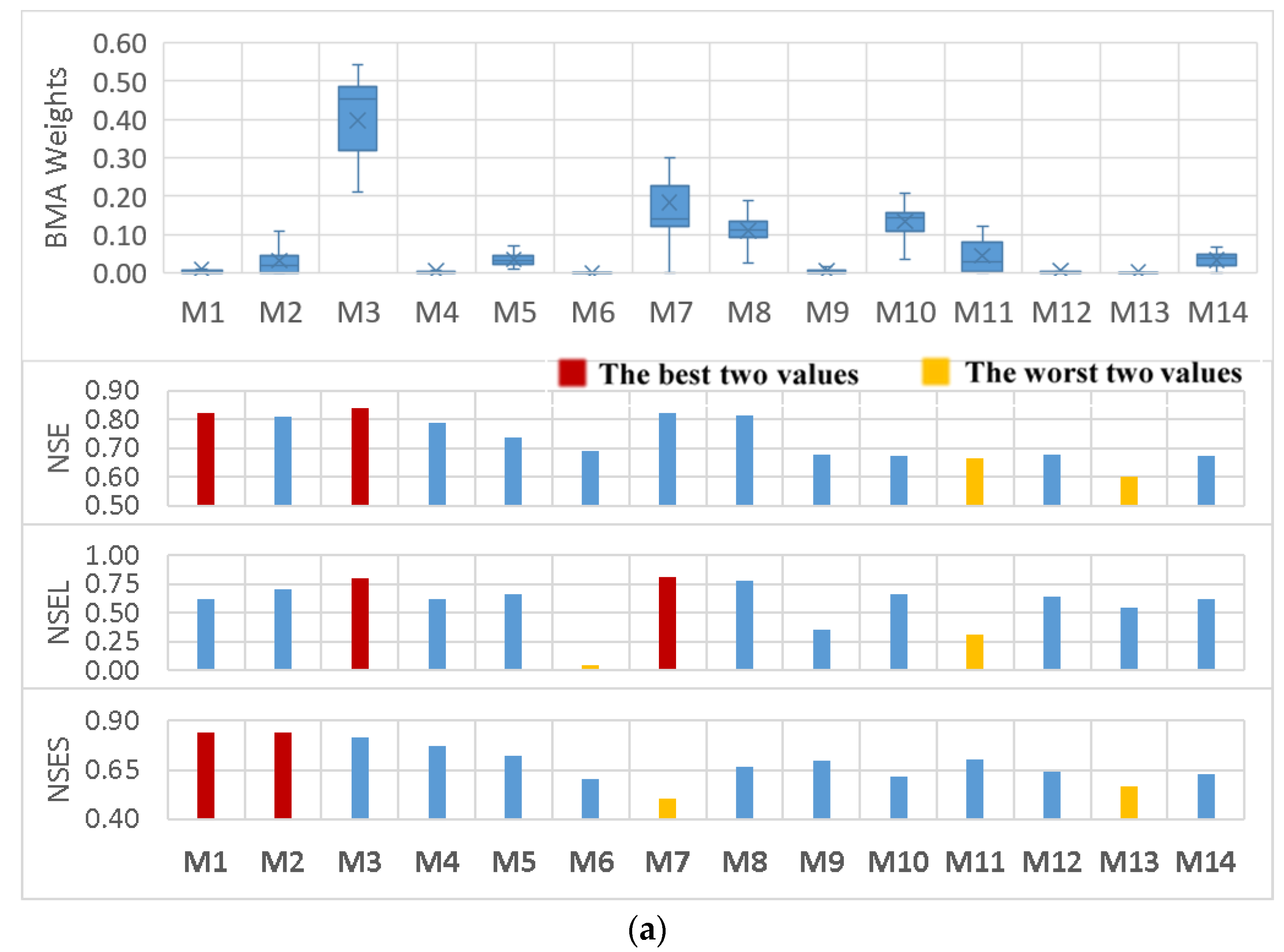
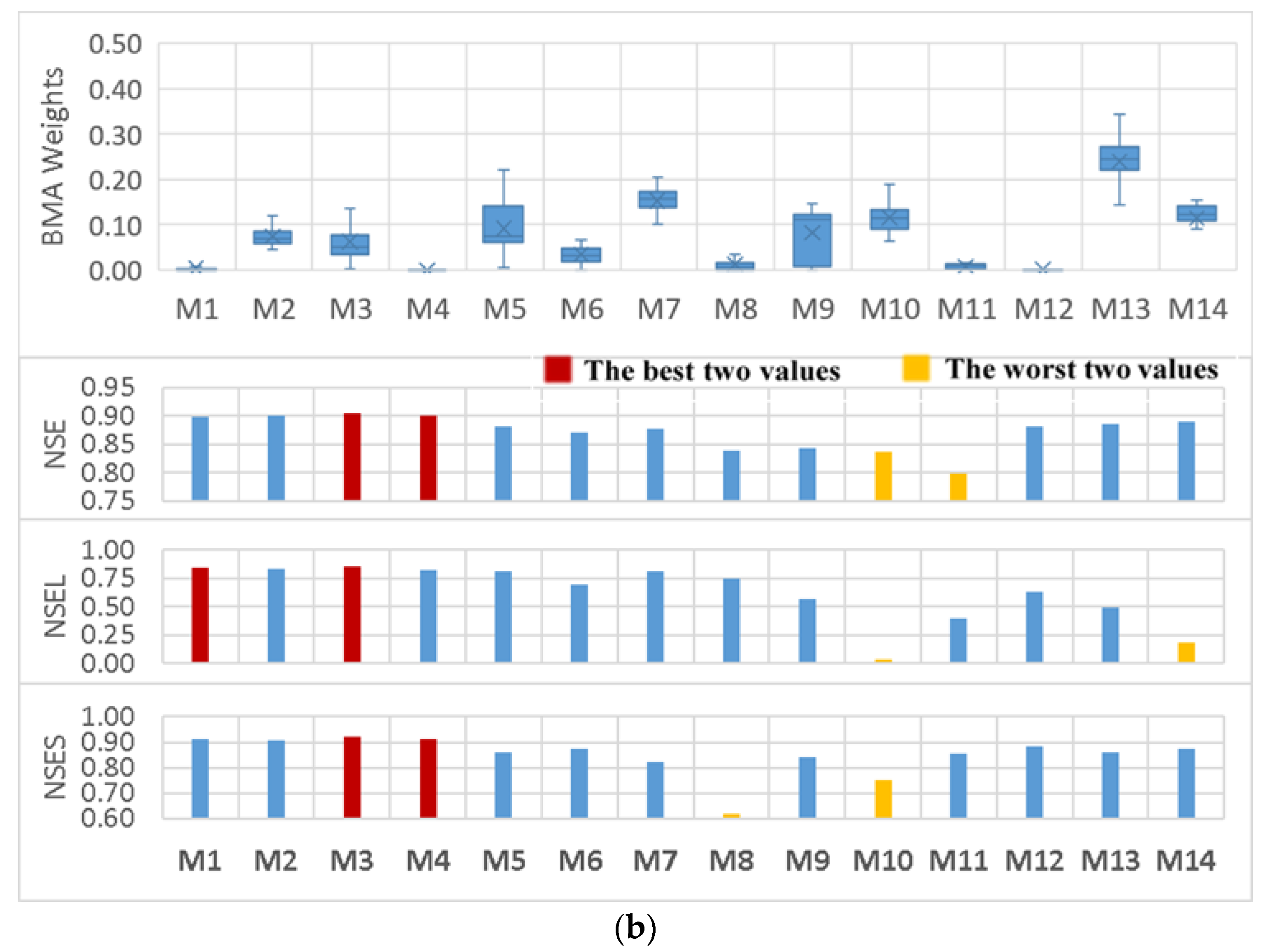
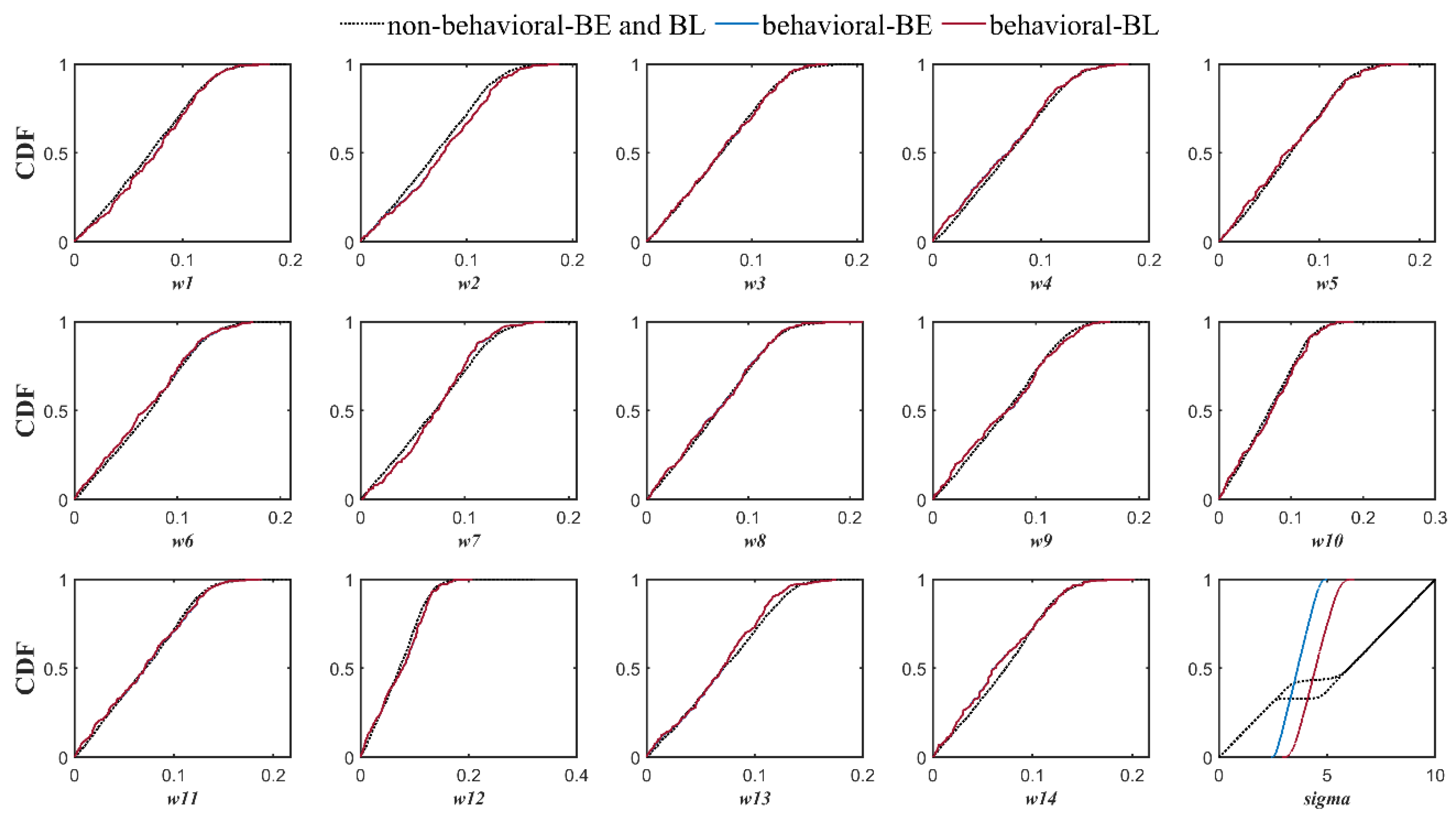
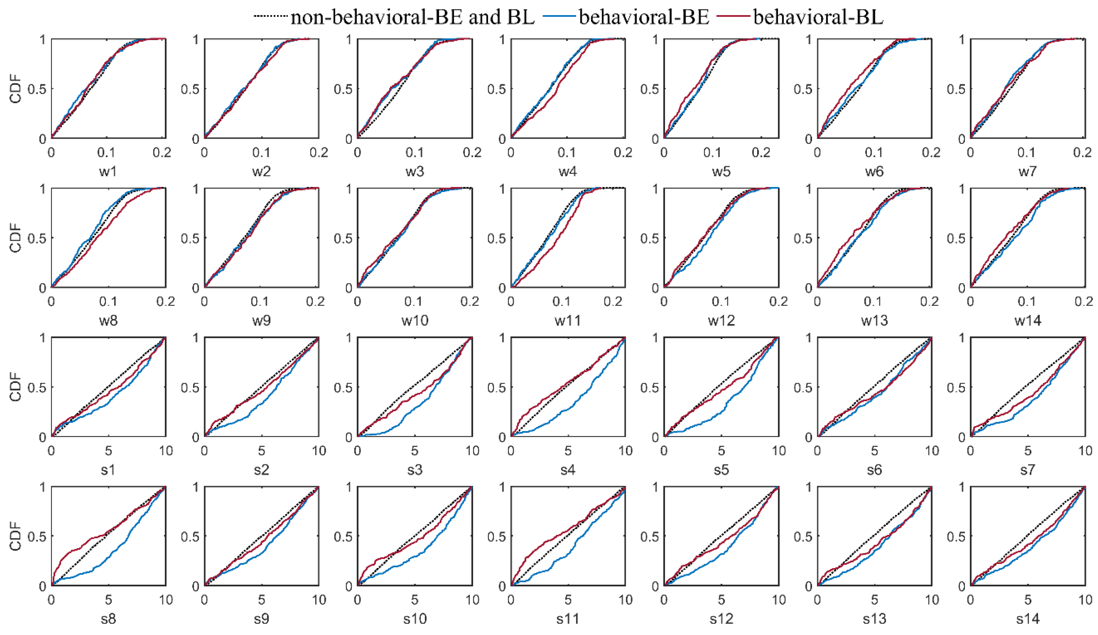
3.2. BMA Weights Versus Models’ Performance Statistics
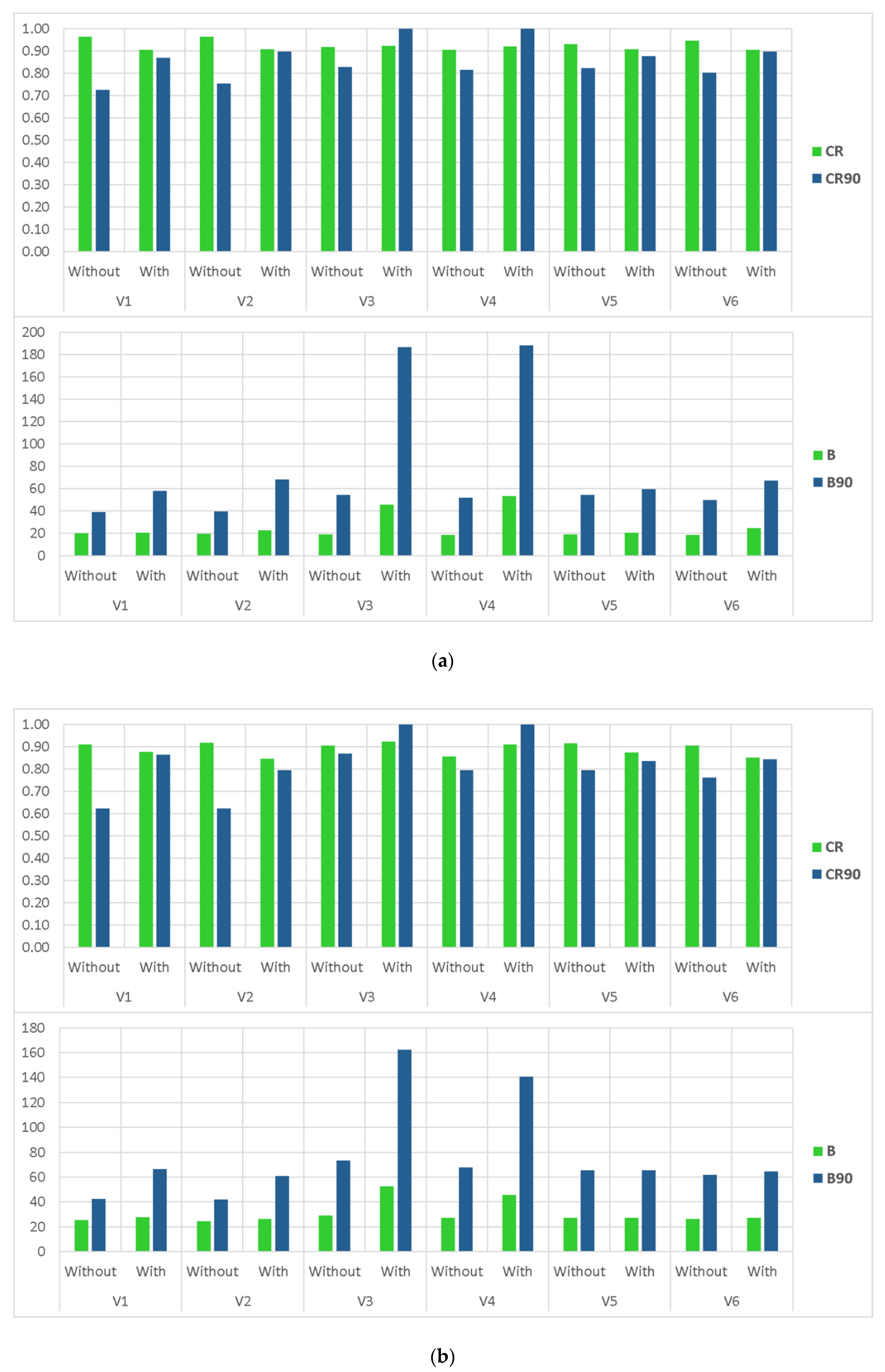
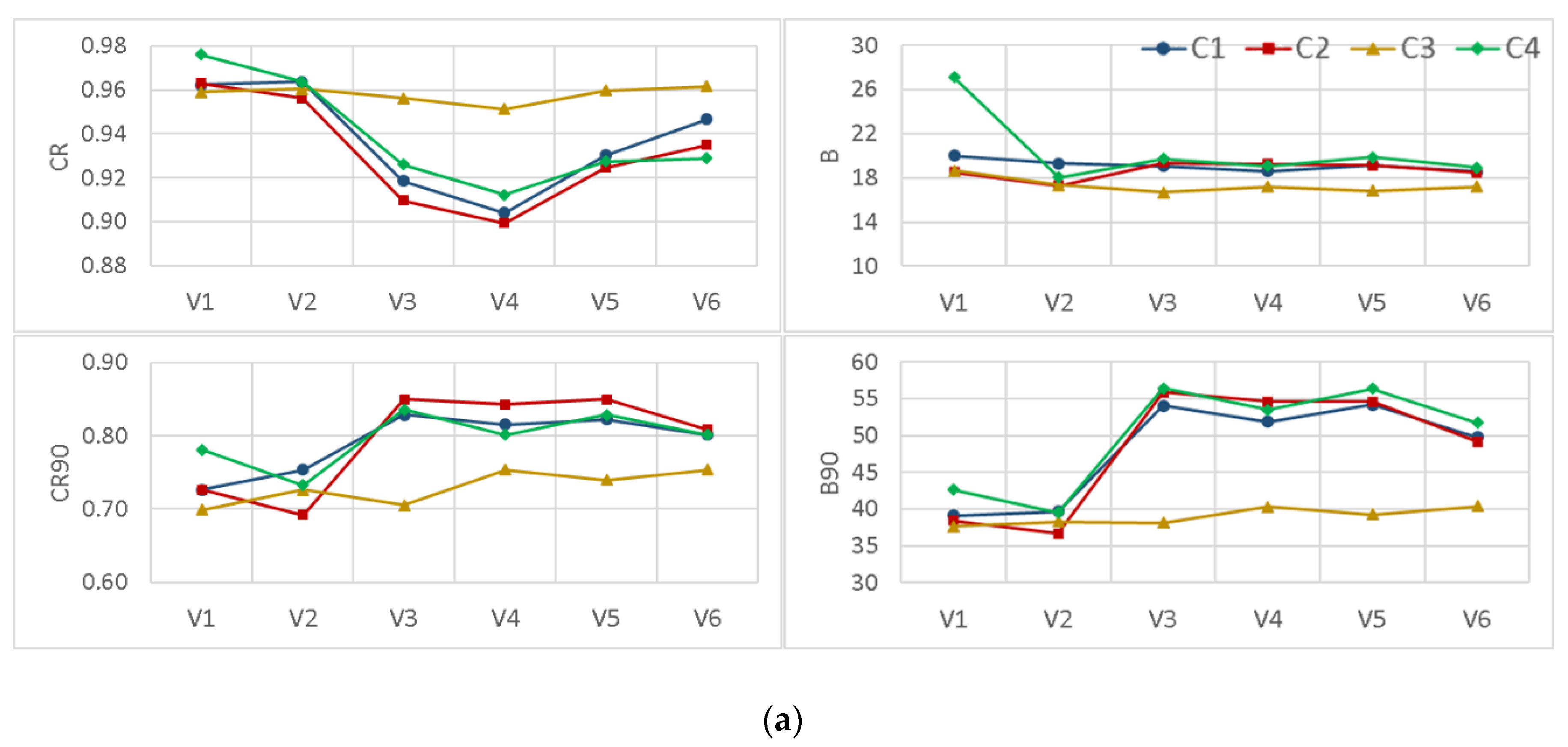
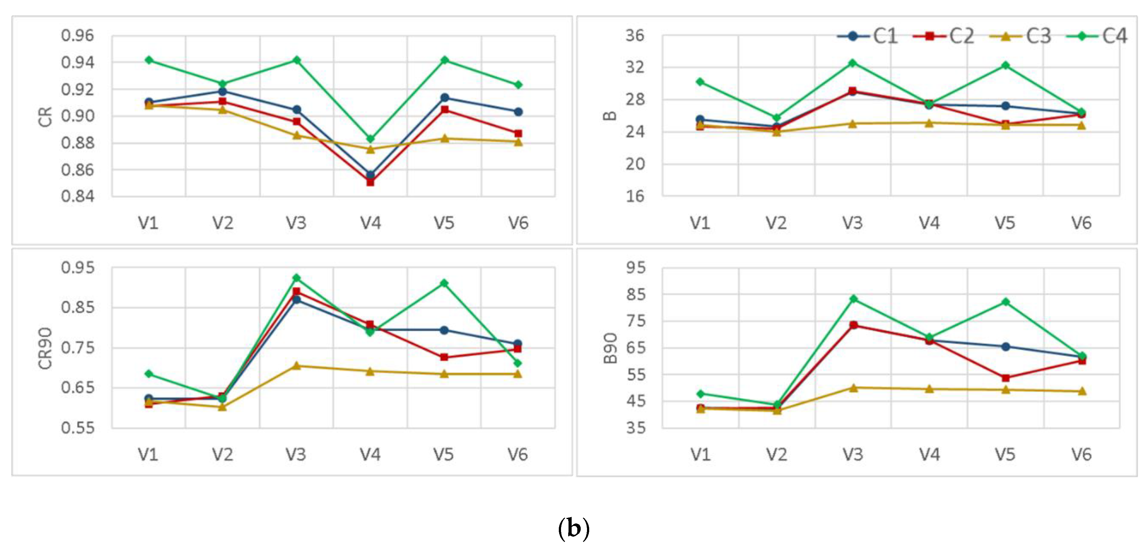
3.3. The Effects of Different Modifications
3.4. Expectation-Maximization Algorithm Versus Dynamically Dimensioned Search Method
4. Summary and Conclusions
- Comparing different ensemble scenarios indicated that, besides using multi-models, considering various forcing precipitation scenarios in generating members of an ensemble leads to better probabilistic and deterministic results in data scarce regions, where the estimation of mean areal precipitation always comes with noticeable errors. However, not only using a multi-model multi-parameter scenario did not provide better results, it also slightly reduced the reliability of the BMA simulations.
- In contrast to earlier findings, however, the results showed that the BMA weights were not completely in accordance with individual model performance. There were some highly weighted hydrologic models with relatively lower performance in comparison to the others in both watersheds. In addition, various BMA modifications led to different combinations of weights and all had almost the same predictive power.
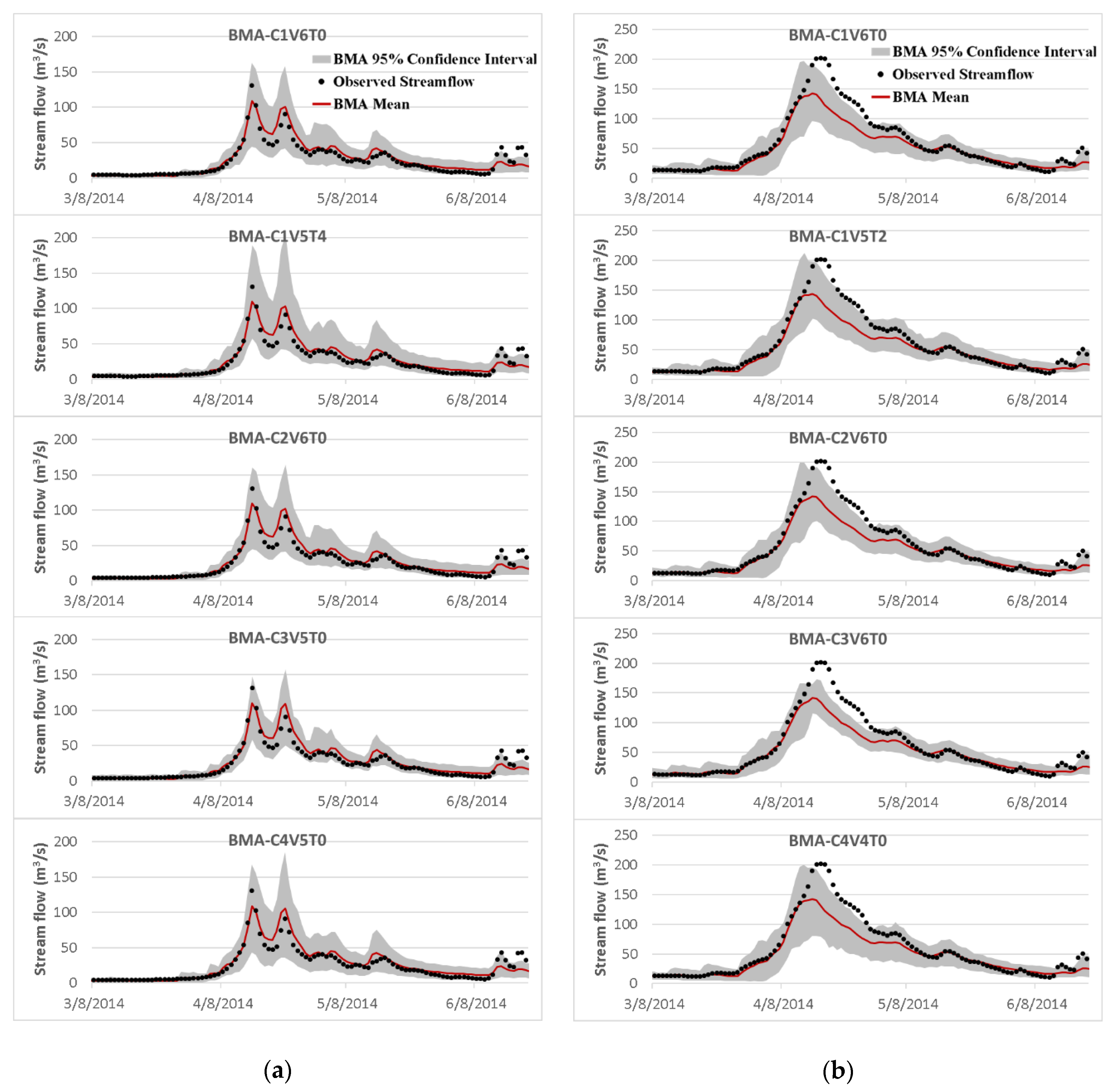
- Applying data transformation generally yielded an improvement in the reliability of the BMA results. However, except for the empirical normal quantile approach, using other data transformation methods concurrent with implementing non-constant standard deviation without a constant parameter dramatically deteriorated the sharpness of the results, specifically in high flows.
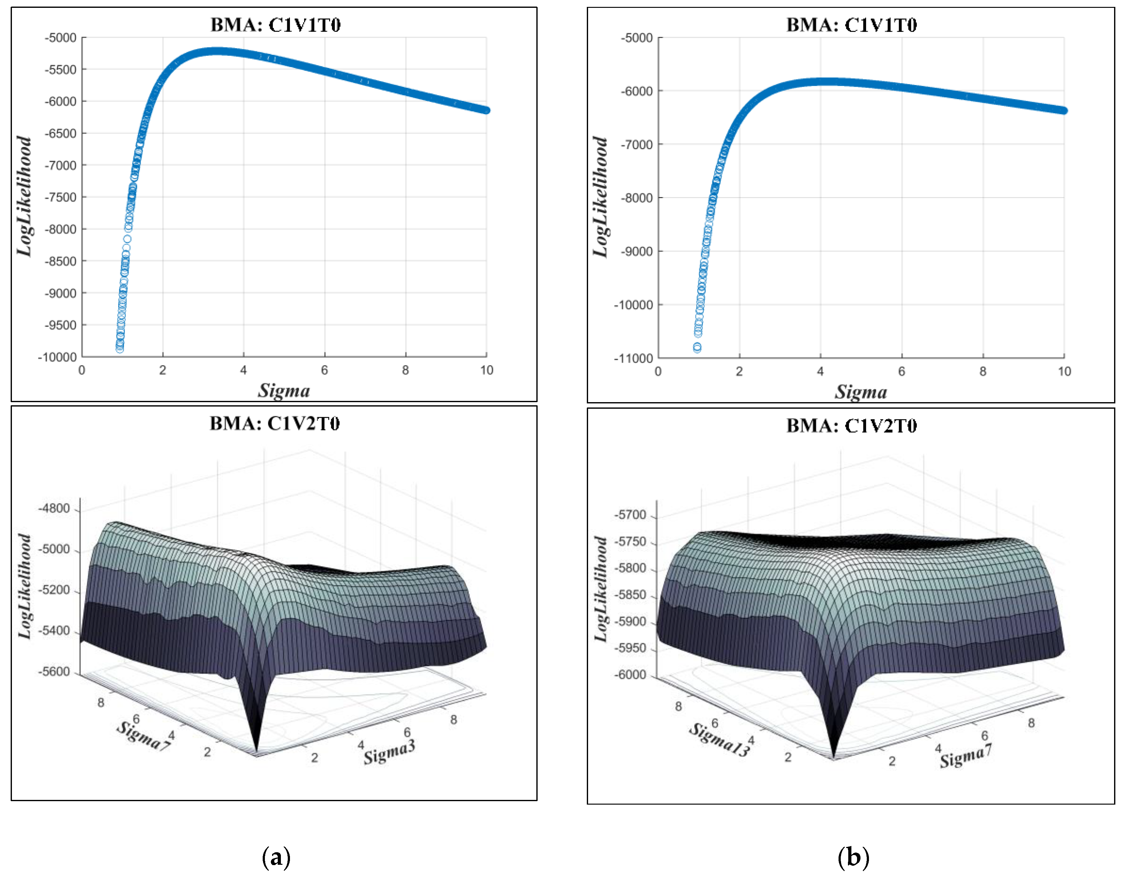
- Incorporation of the more representative distribution types did not show a particular superiority over the classic BMA method, where the posterior predictive distributions were assumed to be Gaussian. However, implementing non-constant standard deviations enhanced the predictive capability of the BMA model, especially for high flows that are often of particular attention in operational hydrology.
- The expectation-maximization algorithm provided almost the same results as the dynamically dimensioned search (DSS) method, which showed its ability to estimate BMA parameters well enough. However, the only drawback was that it could not easily be applied for all BMA variants when the distribution or standard deviation types were changed.
Author Contributions
Funding
Acknowledgments
Conflicts of Interest
References
- Chen, X.; Yang, T.; Wang, X.; Xu, C.Y.; Yu, Z. Uncertainty intercomparison of different hydrological models in simulating extreme flows. Water Resour. Manag. 2013, 27, 1393–1409. [Google Scholar] [CrossRef]
- Liu, Z.; Guo, S.; Zhang, H.; Liu, D.; Yang, G. Comparative study of three updating procedures for real-time flood forecasting. Water Resour. Manag. 2016, 30, 2111–2126. [Google Scholar] [CrossRef]
- Moradkhani, H.; Sorooshian, S. General review of rainfall-runoff modeling: Model calibration, data assimilation, and uncertainty analysis. In Hydrological Modelling and the Water Cycle: Coupling the Atmospheric and Hydrological Models; Sorooshian, S., Hsu, K.L., Coppola, E., Tomassetti, B., Verdecchia, M., Visconti, G., Eds.; Springer: Berlin/Heidelberg, Germany, 2008; Volume 63, pp. 1–24. ISBN 978-3-540-77843-1. [Google Scholar]
- Shrestha, D.L. Uncertainty Analysis in Rainfall-Runoff Modelling—Application of Machine Learning Techniques: UNESCO-IHE. PhD Thesis, IHE Delft Institute for Water Education, Delft, The Netherlands, 2009. [Google Scholar]
- Madadgar, S.; Moradkhani, H. Improved bayesian multimodeling: Integration of copulas and bayesian model averaging. Water Resour. Res. 2014, 50, 9586–9603. [Google Scholar] [CrossRef]
- Michaels, S. Probabilistic forecasting and the reshaping of flood risk management. J. Nat. Resour. Policy Res. 2015, 7, 41–51. [Google Scholar] [CrossRef]
- Seo, D.J.; Herr, H.D.; Schaake, J.C. A statistical post-processor for accounting of hydrologic uncertainty in short-range ensemble streamflow prediction. Hydrol. Earth Syst. Sci. Discuss. 2006, 3, 1987–2035. [Google Scholar] [CrossRef]
- Georgakakos, K.P.; Seo, D.J.; Gupta, H.; Schaake, J.; Butts, M.B. Towards the characterization of streamflow simulation uncertainty through multimodel ensembles. J. Hydrol. 2004, 298, 222–241. [Google Scholar] [CrossRef]
- Vrugt, J.A.; Robinson, B.A. Treatment of uncertainty using ensemble methods: Comparison of sequential data assimilation and Bayesian model averaging. Water Resour. Res. 2007, 4. [Google Scholar] [CrossRef]
- Granger, C.W.; Ramanathan, R. Improved methods of combining forecasts. J. Forecast. Pre-1986 Chichester 1984, 3, 197–204. [Google Scholar] [CrossRef]
- Shamseldin, A.Y.; O’Connor, K.M. A real-time combination method for the outputs of different rainfall-runoff models. Hydrol. Sci. J. 1999, 44, 895–912. [Google Scholar] [CrossRef]
- Shamseldin, A.Y.; O’Connor, K.M.; Liang, G.C. Methods for combining the outputs of different rainfall–runoff models. J. Hydrol. 1997, 197, 203–229. [Google Scholar] [CrossRef]
- Hoeting, J.A.; Madigan, D.; Raftery, A.E.; Volinsky, C.T. Bayesian model averaging: A tutorial. Stat. Sci. 1999, 14, 382–401. [Google Scholar]
- Raftery, A.E. Bayesian model selection in structural equation models. In Testing Structural Equation Models; SAGE: Thousand Oaks, CA, USA, 1993; Volume 154, pp. 163–180. [Google Scholar]
- Raftery, A.E.; Madigan, D.; Hoeting, J.A. Bayesian model averaging for linear regression models. J. Am. Stat. Assoc. 1997, 92, 179–191. [Google Scholar] [CrossRef]
- Raftery, A.E.; Gneiting, T.; Balabdaoui, F.; Polakowski, M. Using bayesian model averaging to calibrate forecast ensembles. Mon. Weather Rev. 2005, 133, 1155–1174. [Google Scholar] [CrossRef]
- Arsenault, R.; Gatien, P.; Renaud, B.; Brissette, F.; Martel, J.L. A comparative analysis of 9 multi-model averaging approaches in hydrological continuous streamflow simulation. J. Hydrol. 2015, 529, 754–767. [Google Scholar] [CrossRef]
- Viallefont, V.; Raftery, A.E.; Richardson, S. Variable selection and Bayesian model averaging in case-control studies. Stat. Med. 2001, 20, 3215–3230. [Google Scholar] [CrossRef] [PubMed]
- Tian, Y.; Booij, M.J.; Xu, Y.P. Uncertainty in high and low flows due to model structure and parameter errors. Stoch. Environ. Res. Risk Assess. 2014, 28, 319–332. [Google Scholar] [CrossRef]
- Liu, J.; Xie, Z. BMA probabilistic quantitative precipitation forecasting over the huaihe basin using TIGGE multimodel ensemble forecasts. Mon. Weather Rev. 2014, 142, 1542–1555. [Google Scholar] [CrossRef]
- Ma, Y.; Hong, Y.; Chen, Y.; Yang, Y.; Tang, G.; Yao, Y.; Long, D.; Li, C.; Han, Z.; Liu, R. Performance of optimally merged multisatellite precipitation products using the dynamic bayesian model averaging scheme over the Tibetan plateau. J. Geophys. Res. Atmospheres 2018, 123, 814–834. [Google Scholar] [CrossRef]
- Sloughter, J.M.L.; Raftery, A.E.; Gneiting, T.; Fraley, C. Probabilistic quantitative precipitation forecasting using bayesian model averaging. Mon. Weather Rev. 2007, 135, 3209–3220. [Google Scholar] [CrossRef]
- Sun, R.; Yuan, H.; Yang, Y. Using multiple satellite-gauge merged precipitation products ensemble for hydrologic uncertainty analysis over the Huaihe River basin. J. Hydrol. 2018, 566, 406–420. [Google Scholar] [CrossRef]
- Neuman, S.P. Maximum likelihood Bayesian averaging of uncertain model predictions. Stoch. Environ. Res. Risk Assess. 2003, 17, 291–305. [Google Scholar] [CrossRef]
- Rojas, R.; Feyen, L.; Dassargues, A. Conceptual model uncertainty in groundwater modeling: Combining generalized likelihood uncertainty estimation and Bayesian model averaging. Water Resour. Res. 2008, 44. [Google Scholar] [CrossRef]
- Zeng, X.; Wu, J.; Wang, D.; Zhu, X.; Long, Y. Assessing Bayesian model averaging uncertainty of groundwater modeling based on information entropy method. J. Hydrol. 2016, 538, 689–704. [Google Scholar] [CrossRef]
- Yan, H.; Moradkhani, H. Toward more robust extreme flood prediction by Bayesian hierarchical and multimodeling. Nat. Hazards 2016, 81, 203–225. [Google Scholar] [CrossRef]
- Ajami, N.K.; Duan, Q.; Sorooshian, S. An integrated hydrologic Bayesian multimodel combination framework: Confronting input, parameter, and model structural uncertainty in hydrologic prediction. Water Resour. Res. 2007, 43. [Google Scholar] [CrossRef]
- Dong, L.; Xiong, L.; Zheng, Y. Uncertainty analysis of coupling multiple hydrologic models and multiple objective functions in Han River, China. Water Sci. Technol. 2013, 68, 506–513. [Google Scholar] [CrossRef] [PubMed]
- Duan, Q.; Ajami, N.K.; Gao, X.; Sorooshian, S. Multi-model ensemble hydrologic prediction using Bayesian model averaging. Adv. Water Resour. 2007, 30, 1371–1386. [Google Scholar] [CrossRef]
- Huo, W.; Li, Z.; Wang, J.; Yao, C.; Zhang, K.; Huang, Y. Multiple hydrological models comparison and an improved Bayesian model averaging approach for ensemble prediction over semi-humid regions. Stoch. Environ. Res. Risk Assess. 2019, 33, 217–238. [Google Scholar] [CrossRef]
- Liang, Z.; Wang, D.; Guo, Y.; Zhang, Y.; Dai, R. Application of Bayesian model averaging approach to multimodel ensemble hydrologic forecasting. J. Hydrol. Eng. 2013, 18, 1426–1436. [Google Scholar] [CrossRef]
- Najafi, M.R.; Moradkhani, H. Ensemble combination of seasonal streamflow forecasts. J. Hydrol. Eng. 2016, 21, 04015043. [Google Scholar] [CrossRef]
- Qu, B.; Zhang, X.; Pappenberger, F.; Zhang, T.; Fang, Y. Multi-model grand ensemble hydrologic forecasting in the Fu River Basin using Bayesian model averaging. Water 2017, 9, 74. [Google Scholar] [CrossRef]
- Yen, H.; Wang, X.; Fontane, D.G.; Harmel, R.D.; Arabi, M. A framework for propagation of uncertainty contributed by parameterization, input data, model structure, and calibration/validation data in watershed modeling. Environ. Model. Softw. 2014, 54, 211–221. [Google Scholar] [CrossRef]
- Todini, E. A model conditional processor to assess predictive uncertainty in flood forecasting. Int. J. River Basin Manag. 2008, 6, 123–137. [Google Scholar] [CrossRef]
- Vrugt, J.A. MODELAVG: A MATLAB Toolbox for Postprocessing of Model Ensembles; Department of Civil and Environmental Engineering, University of California Irvine: Irvine, CA, USA, 2016; Available online: http://faculty.sites.uci.edu/jasper/files/2016/04/manual_Model_averaging.pdf (accessed on 15 August 2019).
- McLachlan, G.; Krishnan, T. The EM Algorithm and Extensions, 2nd ed.; Wiley-Interscience: Hoboken, NJ, USA, 2008; ISBN 978-0-471-20170-0. [Google Scholar]
- Ebtehaj, M.; Moradkhani, H.; Gupta, H.V. Improving robustness of hydrologic parameter estimation by the use of moving block bootstrap resampling: Hydrologic parameter estimation. Water Resour. Res. 2010, 46. [Google Scholar] [CrossRef]
- Vrugt, J.A.; Diks, C.G.H.; Clark, M.P. Ensemble Bayesian model averaging using Markov Chain Monte Carlo sampling. Environ. Fluid Mech. 2008, 8, 579–595. [Google Scholar] [CrossRef]
- Zhang, X.; Srinivasan, R.; Bosch, D. Calibration and uncertainty analysis of the SWAT model using genetic algorithms and Bayesian model averaging. J. Hydrol. 2009, 374, 307–317. [Google Scholar] [CrossRef]
- Meira Neto, A.; Oliveira, P.T.S.; Rodrigues, D.B.; Wendland, E. Improving streamflow prediction using uncertainty analysis and Bayesian model averaging. J. Hydrol. Eng. 2018, 23, 05018004. [Google Scholar] [CrossRef]
- Strauch, M.; Bernhofer, C.; Koide, S.; Volk, M.; Lorz, C.; Makeschin, F. Using precipitation data ensemble for uncertainty analysis in SWAT streamflow simulation. J. Hydrol. 2012, 414, 413–424. [Google Scholar] [CrossRef]
- Parrish, M.A.; Moradkhani, H.; DeChant, C.M. Toward reduction of model uncertainty: Integration of Bayesian model averaging and data assimilation. Water Resour. Res. 2012, 48. [Google Scholar] [CrossRef]
- He, S.; Guo, S.; Liu, Z.; Yin, J.; Chen, K.; Wu, X. Uncertainty analysis of hydrological multi-model ensembles based on CBP-BMA method. Hydrol. Res. 2018, 49, 1636–1651. [Google Scholar] [CrossRef]
- Lespinas, F.; Fortin, V.; Roy, G.; Rasmussen, P.; Stadnyk, T. Performance evaluation of the Canadian precipitation analysis (CaPA). J. Hydrometeorol. 2015, 16, 2045–2064. [Google Scholar] [CrossRef]
- Boluwade, A.; Zhao, K.Y.; Stadnyk, T.A.; Rasmussen, P. Towards validation of the Canadian precipitation analysis (CaPA) for hydrologic modeling applications in the Canadian Prairies. J. Hydrol. 2018, 556, 1244–1255. [Google Scholar] [CrossRef]
- American Society of Civil Engineers. Task committee on hydrology handbook. In Hydrology Handbook; ASCE: New York, NY, USA, 1996; ISBN 978-0-7844-0138-5. [Google Scholar]
- Thiessen, A.H. Precipitation averages for large areas. Mon. Weather Rev. 1911, 39, 1082–1089. [Google Scholar] [CrossRef]
- Box, G.E.P.; Cox, D.R. An analysis of transformations. J. R. Stat. Soc. Ser. B Methodol. 1964, 26, 211–252. [Google Scholar] [CrossRef]
- Krzysztofowicz, R. Transformation and normalization of variates with specified distributions. J. Hydrol. 1997, 197, 286–292. [Google Scholar] [CrossRef]
- Tolson, B.A.; Shoemaker, C.A. Dynamically dimensioned search algorithm for computationally efficient watershed model calibration. Water Resour. Res. 2007, 43. [Google Scholar] [CrossRef]
- Scharffenberg, W. HEC-HMS User’s Manual; Version 4.2; U.S. Army Corps of Engineers Institute for Water Resources Hydrologic Engineering Center (CEIWR-HEC): Davis, CA, USA, 2016. [Google Scholar]
- Refsgaard, J.C.; Knudsen, J. Operational validation and intercomparison of different types of hydrological models. Water Resour. Res. 1996, 32, 2189–2202. [Google Scholar] [CrossRef]
- Tegegne, G.; Park, D.K.; Kim, Y.O. Comparison of hydrological models for the assessment of water resources in a data-scarce region, the Upper Blue Nile River Basin. J. Hydrol. Reg. Stud. 2017, 14, 49–66. [Google Scholar] [CrossRef]
- Anshuman, A.; Kunnath-Poovakka, A.; Eldho, T.I. Towards the use of conceptual models for water resource assessment in Indian tropical watersheds under monsoon-driven climatic conditions. Environ. Earth Sci. 2019, 78, 282. [Google Scholar] [CrossRef]
- Thornthwaite, C.W. An approach toward a rational classification of climate. Geogr. Rev. 1948, 38, 55–94. [Google Scholar] [CrossRef]
- Samuel, J.; Coulibaly, P.; Metcalfe, R.A. Estimation of continuous streamflow in Ontario Ungauged Basins: Comparison of regionalization methods. J. Hydrol. Eng. 2011, 16, 447–459. [Google Scholar] [CrossRef]
- Hargreaves, G.H.; Samani, Z.A. Reference crop evapotranspiration from temperature. Appl. Eng. Agric. 1985, 1, 96–99. [Google Scholar] [CrossRef]
- Anderson, E.A. Snow accumulation and ablation model—SNOW-17. Natl. Ocean. Atmospheric Adm. Natl. Weather Serv. Silver Springs MD 2006. Available online: https://www.nws.noaa.gov/oh/hrl/nwsrfs/users_manual/part2/_pdf/22snow17.pdf (accessed on 15 August 2019).
- Anderson, E.A. National Weather Service River Forecast System: Snow Accumulation and Ablation Model; U.S. Department of Commerce, National Oceanic and Atmospheric Administration, National Weather Service: Washington, DC, USA, 1973.
- Rabi, G.; Watkins David, W. Continuous hydrologic modeling of snow-affected watersheds in the great lakes basin using HEC-HMS. J. Hydrol. Eng. 2013, 18, 29–39. [Google Scholar] [CrossRef]
- Agnihotri, J. Evaluation of Snowmelt Estimation Techniques for Enhanced Spring Peak Flow Prediction. Master’s Thesis, McMaster University, Hamilton, ON, Canada, 2018. [Google Scholar]
- Burnash, R.J.C.; Ferral, R.L.; McGuire, R.A. A Generalized Streamflow Simulation System: Conceptual Modeling for Digital Computers; Joint Federal-State River Forecast Center, United States National Weather Service: Los Angeles, CA, USA, 1973. [Google Scholar]
- Samuel, J.; Coulibaly, P.; Metcalfe, R.A. Identification of rainfall–runoff model for improved baseflow estimation in ungauged basins. Hydrol. Process. 2012, 26, 356–366. [Google Scholar] [CrossRef]
- Tan, B.Q.; O’Connor, K.M. Application of an empirical infiltration equation in the SMAR conceptual model. J. Hydrol. 1996, 185, 275–295. [Google Scholar] [CrossRef]
- Nascimento, N.D.E.O.; Yang, X.L.; Makhlouf, Z.; Michel, C. GR3J: A daily watershed model with three free parameters. Hydrol. Sci. J. 1999, 44, 263–277. [Google Scholar]
- Nash, J.E.; Sutcliffe, J.V. River flow forecasting through conceptual models part I—A discussion of principles. J. Hydrol. 1970, 10, 282–290. [Google Scholar] [CrossRef]
- Gupta, H.V.; Kling, H.; Yilmaz, K.K.; Martinez, G.F. Decomposition of the mean squared error and NSE performance criteria: Implications for improving hydrological modelling. J. Hydrol. 2009, 377, 80–91. [Google Scholar] [CrossRef]
- Cunderlik, J.; Simonovic, S. Calibration, Verification and Sensitivity Analysis of the HEC-HMS Hydrologic Model; Department of Civil and Environmental Engineering, The University of Western Ontario: London, ON, Canada, 2004. [Google Scholar]
- Xiong, L.; Wan, M.; Wei, X.; O’Connor, K.M. Indices for assessing the prediction bounds of hydrological models and application by generalised likelihood uncertainty estimation/Indices pour évaluer les bornes de prévision de modèles hydrologiques et mise en œuvre pour une estimation d’incertitude par vraisemblance généralisée. Hydrol. Sci. J. 2009, 54, 852–871. [Google Scholar]
- Hornberger, G.M.; Spear, R.C. Approach to the preliminary analysis of environmental systems. J. Environ. Manag. 1981, 12, 7–18. [Google Scholar]


| Streamflow Ensemble | Data Transformation Method | Distribution Type | Standard Deviation Type | Optimization Method |
|---|---|---|---|---|
| Multi-Model(M-M1) | No Transformation (T0) | Normal (C1) | Common Constant (V1) | Expectation-Maximization Algorithm (EM) |
| Multi-Model Multi-Input (M-MI) | Box–Cox Type 1 (T1) | Gamma (C2) | Individual Constant (V2) | |
| Multi-Model Multi-Parameter (M-MP) | Box–Cox Type 2 (T2) | Log-Normal (C3) | Common Non-Constant (V3) | Dynamically Dimensioned Search (DDS) |
| Multi-Model Multi-Input Multi-Parameter (M-MIP) | Logarithmic Transform (T3) | Weibull (C4) | Individual Non-Constant (V4) | |
| Empirical Normal Quantile Transform (T4) | Common Non-Constant + Constant Value (V5) | |||
| Individual Non-Constant + Constant Value (V6) |
| Standard Deviation Type | Formulation | BMA Parameters |
|---|---|---|
| Common Constant (V11) | ||
| Individual Constant (V2) | ||
| Common Non-Constant (V3) | ||
| Individual Non-Constant (V4) | ||
| Common Non-Constant Type 2 (V5) | ||
| Individual Non-Constant Type 2 (V6) |
| Model ID | Full Name | Reference | Number of Parameters |
|---|---|---|---|
| SAC-SMA | Sacramento Soil Moisture Accounting | Burnash et al. [64] | 19 |
| MAC-HBV | McMaster University Hydrologiska Byrans Vattenbalansavdelning | Samuel et al. [65] | 15 |
| SMARG | Modified Soil Moisture Accounting and Routing | Tan and O’Connor. [66] | 14 |
| GR4J | Génie Rural à 4 Paramètres Journaliers | Edijatno et al. [67] | 9 |
| HEC-HMS1 | Hydrologic Engineering Center’s Hydrologic Modeling System-Type 1 | USACE-HEC [53] | 17 |
| HEC-HMS2 | Hydrologic Engineering Center’s Hydrologic Modeling System-Type 2 | USACE-HEC [53] | 25 |
| HEC-HMS3 | Hydrologic Engineering Center’s Hydrologic Modeling System-Type 3 | USACE-HEC [53] | 27 |
| Criteria | Big East River Watershed | Black River Watershed | ||||||
|---|---|---|---|---|---|---|---|---|
| M-MIP | M-MP | M-MI | M-M | M-MIP | M-MP | M-MI | M-M | |
| 1 | 0.76 | 0.74 | 0.79 | 0.77 | 0.82 | 0.81 | 0.84 | 0.81 |
| 1 | 0.45 | 0.42 | 0.54 | 0.49 | 0.57 | 0.55 | 0.62 | 0.56 |
| 1 | 0.84 | 0.84 | 0.82 | 0.83 | 0.79 | 0.80 | 0.78 | 0.77 |
| 1 | 0.95 | 0.94 | 0.96 | 0.96 | 0.92 | 0.90 | 0.91 | 0.88 |
| 1 | 17 | 18 | 19 | 23 | 27 | 28 | 24 | 27 |
| 1 | 0.72 | 0.64 | 0.73 | 0.68 | 0.62 | 0.46 | 0.62 | 0.49 |
| 1 | 39 | 32 | 38 | 34 | 55 | 48 | 41 | 36 |
| Basin | Criteria | BMA Variant | |||||||
|---|---|---|---|---|---|---|---|---|---|
| C1V5T1 | C1V5T2 | C1V5T3 | C1V5T4 | C1V4T1 | C1V4T2 | C1V4T3 | C1V4T4 | ||
| BE | 0.91 | 0.90 | 0.91 | 0.90 | 0.92 | 0.93 | 0.92 | 0.91 | |
| 25 | 22 | 21 | 24 | 127 | 73 | 53 | 30 | ||
| 0.90 | 0.88 | 0.88 | 0.89 | 1.00 | 1.00 | 1.00 | 0.98 | ||
| 82 | 65 | 60 | 65 | 720 | 364 | 188 | 87 | ||
| BL | 0.87 | 0.88 | 0.87 | 0.86 | 0.91 | 0.91 | 0.91 | 0.88 | |
| 27 | 27 | 29 | 27 | 46 | 46 | 52 | 30 | ||
| 0.84 | 0.80 | 0.92 | 0.85 | 0.99 | 1.00 | 0.99 | 0.88 | ||
| 66 | 64 | 73 | 64 | 143 | 141 | 170 | 76 | ||
| Criteria | NSE | NSES | NSEL | CR | B | CR90 | B90 | |
|---|---|---|---|---|---|---|---|---|
| Big East River | C1V6T0 | 0.77 | 0.49 | 0.81 | 0.95 | 19 | 0.80 | 50 |
| C1V5T4 | 0.77 | 0.49 | 0.82 | 0.91 | 21 | 0.88 | 60 | |
| C2V6T0 | 0.77 | 0.49 | 0.82 | 0.93 | 18 | 0.81 | 49 | |
| C3V5T0 | 0.78 | 0.54 | 0.83 | 0.96 | 17 | 0.74 | 40 | |
| C4V5T0 | 0.77 | 0.51 | 0.82 | 0.93 | 20 | 0.83 | 56 | |
| Black River | C1V6T0 | 0.83 | 0.60 | 0.80 | 0.90 | 26 | 0.76 | 61 |
| C1V5T2 | 0.83 | 0.59 | 0.80 | 0.87 | 27 | 0.84 | 66 | |
| C2V6T0 | 0.83 | 0.61 | 0.80 | 0.89 | 26 | 0.75 | 60 | |
| C3V6T0 | 0.83 | 0.61 | 0.79 | 0.89 | 25 | 0.71 | 50 | |
| C4V4T0 | 0.83 | 0.59 | 0.80 | 0.88 | 27 | 0.79 | 69 | |
© 2019 by the authors. Licensee MDPI, Basel, Switzerland. This article is an open access article distributed under the terms and conditions of the Creative Commons Attribution (CC BY) license (http://creativecommons.org/licenses/by/4.0/).
Share and Cite
Darbandsari, P.; Coulibaly, P. Inter-Comparison of Different Bayesian Model Averaging Modifications in Streamflow Simulation. Water 2019, 11, 1707. https://doi.org/10.3390/w11081707
Darbandsari P, Coulibaly P. Inter-Comparison of Different Bayesian Model Averaging Modifications in Streamflow Simulation. Water. 2019; 11(8):1707. https://doi.org/10.3390/w11081707
Chicago/Turabian StyleDarbandsari, Pedram, and Paulin Coulibaly. 2019. "Inter-Comparison of Different Bayesian Model Averaging Modifications in Streamflow Simulation" Water 11, no. 8: 1707. https://doi.org/10.3390/w11081707
APA StyleDarbandsari, P., & Coulibaly, P. (2019). Inter-Comparison of Different Bayesian Model Averaging Modifications in Streamflow Simulation. Water, 11(8), 1707. https://doi.org/10.3390/w11081707