Article

Development of Threshold Levels and a Climate-Sensitivity Model of the Hydrological Regime of the High-Altitude Catchment of the Western Himalayas, Pakistan

1
Institute of International Rivers and Eco-Security, Yunnan University, Kunming 650500, China
2
Department of Agricultural Engineering, Muhammad Nawaz Shareef University of Agriculture, Multan 66000, Pakistan
3
Department of Environmental Sciences, COMSATS University Islamabad, Abbottabad campus, Abbottabad 22060, Pakistan
4
Department of Irrigation and Drainage, University of Agriculture, Faisalabad 380000, Pakistan
5
Department of Civil and Environmental Engineering and Construction, University of Nevada, Las Vegas, NV 89154, USA
6
State Key Laboratory of Cryospheric Science, Northwest Institute of Eco-Environment and Resources, Chinese Academy of Sciences (CAS), Lanzhou 730000, China
7
University of Chinese Academy of Sciences, Beijing 100049, China
8
Department of Agricultural Engineering, Khwaja Fareed University of Engineering and Information Technology, Rahim Yar Khan 64200, Pakistan
9
Common Wealth Scientific and Industrial Research Organization Land and Water, Canberra 2601, Australia
10
Key Laboratory of Water Cycle and Related Land Surface Processes, Institute of Geographic Sciences and Natural Resources Research, Chinese Academy of Sciences, Beijing 100101, China
*
Author to whom correspondence should be addressed.
Water 2019, 11(7), 1454; https://doi.org/10.3390/w11071454
Submission received: 18 May 2019 / Revised: 21 June 2019 / Accepted: 9 July 2019 / Published: 14 July 2019
(This article belongs to the Special Issue Evaluating Hydrological Responses to Climate Change)

Abstract

:
Water shortages in Pakistan are among the most severe in the world, and its water resources are decreasing significantly due to the prevailing hydro-meteorological conditions. We assessed variations in meteorological and hydrological variables using innovative trend analysis (ITA) and traditional trend analysis methods at a practical significance level, which is also of practical interest. We developed threshold levels of hydrological variables and developed a non-parametric climate-sensitivity model of the high-altitude catchment of the western Himalayas. The runoff of Zone I decreased, while the temperature increased and the precipitation increased significantly. In Zone II, the runoff and temperature increased but the precipitation decreased. A two-dimensional visualization of the Pardé coefficient showed extreme drought events, and indicated greater sensitivity of the hydrological regime to temperature than to precipitation. The threshold levels of runoff for Zones I and II were 320 and 363 mm using the Q80 fixed method, while the mean runoff amounts were estimated to be 79.95 and 55.61 mm, respectively. The transient threshold levels varied by month, and the duration of droughts in Zones I and II ranged from 26.39 to 78.98 days. The sensitivity of the hydrological regime was estimated based on a modified climate-elasticity model (εp = 0.11–0.23, εt = −0.04–2.39) for Zones I and II, respectively. These results highlight the sensitivity of the hydrological regime to temperature, which influences the melting process. However, it is important to establish thresholds for hydrological variables and understand the climate sensitivity of the hydrological regime of the entire basin, so that policy makers and water managers can make sustainable water-resource-management decisions for this region.

Graphical Abstract

1. Introduction

Water is extremely important to all human beings, and is also necessary for a country’s agricultural, industrial, and socioeconomic development. There is a discontinuous layer of water on the surface of the Earth, known as the hydrosphere. Concentrations of greenhouse gases in the atmosphere are increasing, causing global warming and affecting precipitation [1]. These principle factors, i.e., precipitation and temperature, affect the hydrosphere due to their influence on snow [2] and glacial melt [3], which in turn affect runoff to major rivers [4,5,6], the levels of which have changed significantly [7,8,9,10]. The increase in water shortage crises has led to a number of water-related disasters around the world [11,12]. Motivated by these extreme events, the threshold levels of runoff have been determined by various researchers worldwide [13,14]. The duration and severity of droughts is determined based on fixed and monthly thresholds for a given time series [15]. The sensitivity of runoff to climate variation [16], and the runoff thresholds [14], have been analyzed to identify drought events [17] according to the hydrological regime. This has been a major area of interest for global hydrology researchers over the last decade [6,18,19]. The authors of [20] described a hydrological drought as “a significant decrease in the availability of water in all its forms, appearing in the land phase of the hydrological cycle.” Different approaches are widely used in drought analyses [14,17,21,22,23,24]. The authors of [25] used variable thresholds to analyze seasonal, monthly, and daily stream flows. Similarly, the authors of [14] reported that the stream-flow threshold is a key variable for describing hydrological droughts, based on each component of the hydrological cycle. The threshold levels at Q80, Q70 and Q90 have been evaluated to identify drought events with different durations. Stream flow is the main water source for several water-dependent activities, such as hydropower generation, recreation, and irrigation for agriculture. For the purpose of sustainable water-resource management, it is necessary to establish threshold levels and understand the relationship between precipitation and temperature within a hydrological regime [26,27]. Precipitation and temperature are considered to contribute significantly to variations in a given hydrological regime [28,29]. Different methods have been applied to assess the climate sensitivity of hydrological regimes using both parametric and non-parametric approaches [5,30,31]. These methods can be classified as follows: paired-catchment, statistical, and hydrological modeling methods. The drawback of the paired-catchment method is that it is difficult and expensive to identify two catchments with similar characteristics. A large set of parameters is required to apply the hydrological-modeling method, in which these parameters are used to calibrate and validate the model. This makes it difficult to model basins in data-scarce regions [32,33,34]. The Budyko framework is considered an effective tool for assessing the sensitivity of a hydrological regime to precipitation and temperature [35,36,37]. This framework has been used successfully for different rivers globally [6,38]. The non-parametric approach shows a clear relationship between precipitation and temperature within a hydrological regime [39]. Hydrological regimes are sensitive to precipitation and temperature in different regions [5,40]. As it is based directly on long-term observational records, climate-sensitivity analysis is generally reliable.
Pakistan’s economy is highly dependent on agriculture, for which water resources are essential. The main tributaries to the Indus river system (IRS) are a number of streams originating from the Tibetan Plateau, the Karakoram, and the Himalayas [41]. One of the major reservoirs in the western Himalayas is the Mangla reservoir, which is used for irrigation, water supply and hydropower generation. The installed capacity of the Mangla power plant is 1000 MW. The contribution from the western Himalayas, which provide 20–40% of the total flow, is in the form of melted snow. The high-altitude catchment of the western Himalayas provides approximately 65% of the water from this region. The economy of the basin is mostly agro-pastoral and the population is entirely rural. Most people are engaged in agriculture and the rearing of animals, and are also adept at living in the nearby mountainous zones. In this region in Pakistan, approximately 93% of the gross annual flow is consumed for agricultural purposes, 5% for manufacturing purposes, and 2% for residential purposes. The water of the high-altitude tributaries in the western Himalayas is frequently used for irrigation and power generation, as well as municipal and refreshment purposes. Due to the high altitude and complex surface topography of the western Himalayas, ground-based and field observation data are inadequate for characterizing the hydrological regime of this region. As mentioned previously, due to the diversity of regions, it is useful to establish threshold levels of runoff sensitivity to the climate in a specific basin, so that water resources can be better planned and managed. Projected future temperature and precipitation trends were determined in the western Himalayas [1]. Similarly, different climate models have been used to predict the impact of future climate change on this region, without taking into account historical meteorological and hydrological time-series data [42,43]. The authors of [44] investigated the temperature and snow-melt process in the western Himalayas. However, no research has applied innovative trend analysis (ITA)-based approaches to analyses of the spatial and temporal characteristics of these processes. We developed a non-parametric method based on the fractional hydrological response to atmospheric variation. Our ITA forecasting and modified non-parametric approach can be applied to regions throughout the world. The development and duration of severe drought events have never been analyzed in terms of threshold levels of variables in the hydrological regime of the high-altitude catchment of the western Himalayas. This catchment is a major source of water for Pakistan. To the best of our knowledge, this study represents the first attempt to evaluate the sensitivity of runoff in this region to precipitation and temperature. The aims of this study are: to determine the spatial and temporal variations in hydrological regime with tradition and modify methods, develop threshold levels for water security, assess the sensitivity of temperature and precipitation to runoff with traditional and modify climate sensitivity methods. Thus, our work will help water-resource managers and planners to develop sustainable water-resource-management techniques.

2. Methodology

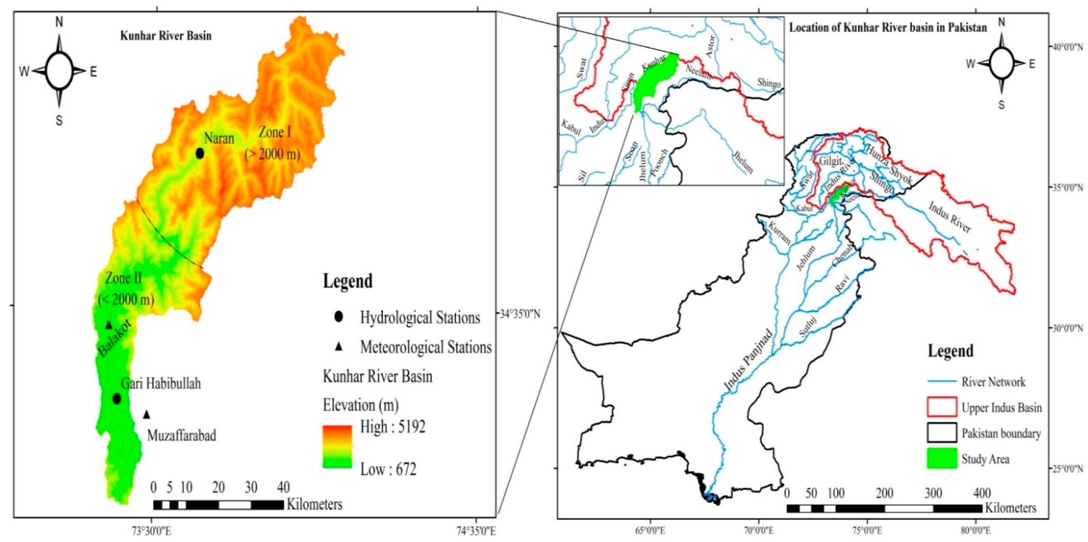
2.1. Study Area and Data Collection

This study was conducted in the Kunhar River basin, a high-altitude catchment in the western Himalayas in Pakistan. The Mangla Dam receives 11% of the Kunhar River flow. Being in the western Himalayas, the major part of this basin, which is at altitudes exceeding 1500 m, receives precipitation from the summer monsoon and winter westerlies. In the case of the area affected by the monsoon, the seasonal precipitation exhibits two peaks. Only one annual peak was detected in the precipitation in the area affected by westerlies, based on records collected from Narran station. A major high-altitude tributary of the western Himalayas is the Kunhar River; its coordinates are 34 N and 74 E, as shown in Figure 1. The Kunhar River starts from the Lulusar Lake in the Kaghaan Valley, in the Khyber Pakhtunkhwa, Pakistan. The river flows through many areas, including Naran, Gari Habibullah, and Balakot, and finally merges with the Jhelum River at Rara, which has a drainage area of approximately 2535 km2.
River flow has been monitored by the Water and Power Development Authority of Pakistan. The Pakistan Meteorological Department (PMD) runs three meteorological stations, and we applied their observation data in this study, including daily historic maximum and minimum temperatures and rainfall (Table 1). The catchment divides the basin into two zones based on elevation: Zone I, which is above 2000 m, and Zone II, which is below 2000 m. Separating the basin into these different zones is important for understanding the meteorological and hydrological conditions.
The normal probability distribution, and mean, median, minimum, maximum, and standard deviation of the precipitation, temperature, and runoff for the two zones are shown in Figure 2 and Figure 3. The average precipitation varied between 120.81 mm (Zone I) and 134.66 mm (Zone II). The average temperature was from 6.35 °C (Zone 1) to 18.67 °C (Zone II). The maximum runoff in both zones occurred during June, when Zone I had 24% more runoff than Zone II. The minimum precipitation was observed during August in Zone I (54.22 mm) and during November in Zone II (43.94 mm). The maximum precipitation occurred in March in Zone I, when it was 29% higher than in Zone II. The maximum temperature of Zone I occurred during July (15.1 °C), whereas the lowest temperature occurred in February (−6.1 °C). The strength of the inter-annual relationship between precipitation and runoff for Zone I was 0.24, which was 44.5% weaker than that for Zone II. Zone I was found to be more sensitive to temperature due to the stronger relationship between temperature and runoff.

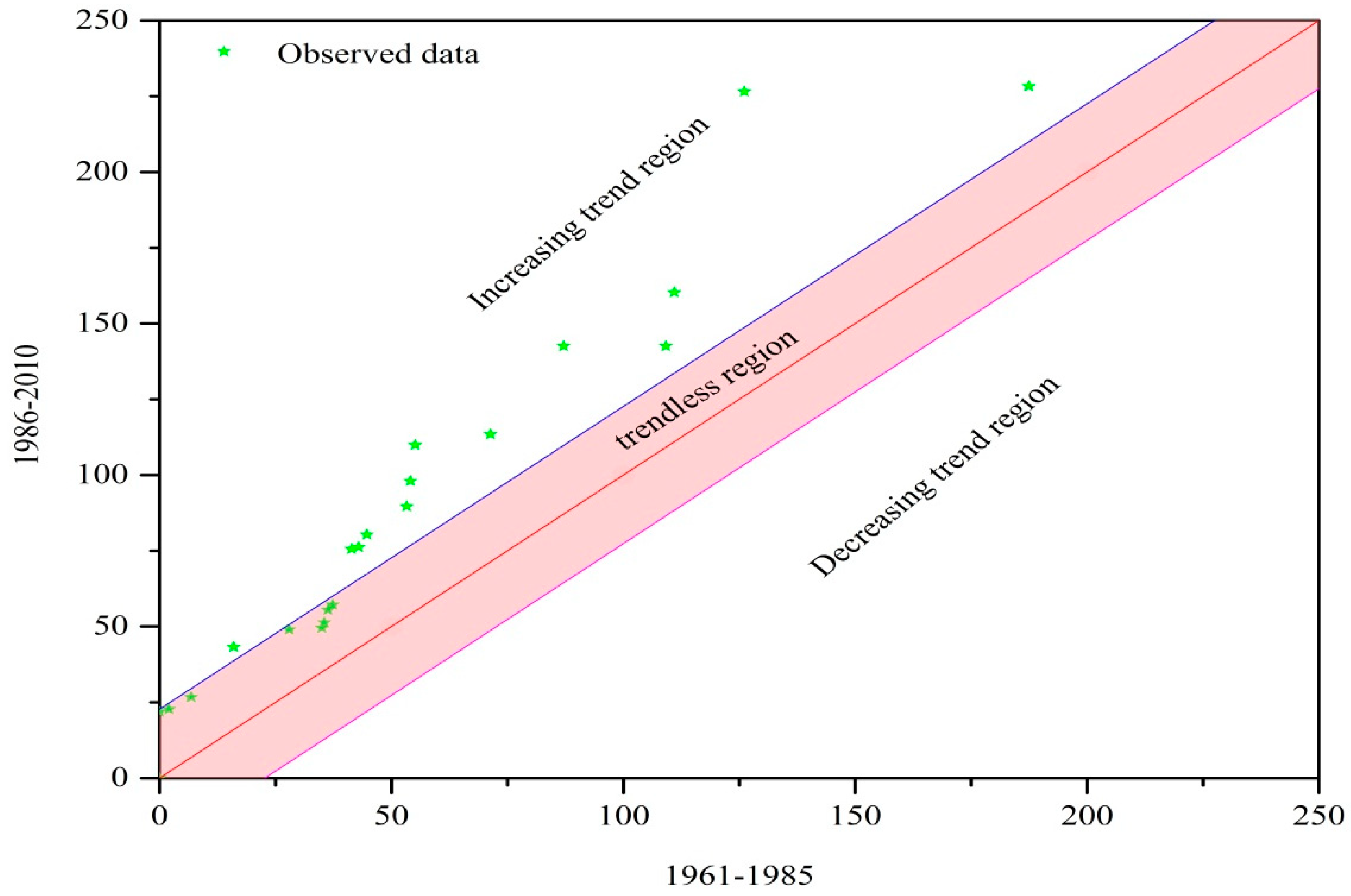
2.2. Innovative Trend Detection Test

The observed time series is divided into subsections and plotted in Cartesian coordinates, which is not dependent on trend, pre-assigned significance level, magnitude, sample size, and variations in time series [16,45]. The observed hydrological time series was divided into two equal parts; these subseries were arranged separately, in ascending order. The first sub-series Xi was then assigned to the X-axis, and the second (Xj) to the Y-axis (Figure 4), of the Cartesian coordinate system. If a hydrological time series follows the 1:1 (45°) straight line, it is termed as trendless. If the data values fall below a straight line (the gradient is less than 45°), there is a decreasing trend. There is an increasing trend if the data values fall above a straight line (the gradient is greater than 45°), [16,46,47]. Whether the points are above or below the 1:1 line denotes whether a trend is increasing or decreasing monotonically.
The average difference between the Xi and Xj values at each point was calculated to assess the increasing and decreasing trends of the given time series. A straight line was drawn at 45°, which represents the trend-less region. The magnitude of the trend was determined based on the first half of the time series. The trend statistics were calculated by dividing the average difference between the data and the line at 45° by the average of the first half of the time series, as follows:
S = 1 n i = 1 n ( X j X i ) X i ¯
where S is the ITA statistic and n is the length of each subseries. Xj and Xi represent, respectively, the second and first subseries for a given time period, and cover the entire basin. Therefore, we compared the ITA statistics to Sen’s slope estimator and carried out a Mann–Kendall (MK) trend test. For this comparison, we scaled the trend statistics by the percentage increase and decrease. In this study, we evaluated the trends such that the results obtained using different approaches and sites were comparable by applying the method recorded in [48]. The percentage variation in the mean of the sample data over the observation period (T) at any site was represented using the same scale as used in the MK test [49] and Sen’s slope estimator [50,51] as described in Appendix A at the 10% significance level and was calculated as follows:
B   ( % ) = T ( β , S ) X ¯ × 100
where T is the observed time period, β is Sen’s slope estimator, S is the ITA statistic and X ¯ is the mean of a given time series. The practical significance of a trend can be defined as percentage increase in sample mean over an observation period. In this study, the practical significance level is set to be 10 percent. This is a trend, which is judged to be of practical interest only when an increase in the mean of sample data over an observation period. Therefore, when a change in sample mean over an observation period is less than 10 percent, this change is considered to be caused by different errors which cannot influence practical importance. The practical significance level is 10%. This significance level is important to water-resource managers and planners.

2.3. Hydrological Regime Variability

One of the best-known methods for hydrological-regime analysis is the Pardé coefficient, which has been applied in numerous studies [52,53]. The Pardé coefficient has numerous advantages over other methods, including that the calculation is simple and based on a normal data sequence, although this does not permit unbiased comparison. This method enables calculation of the normalized coefficients of hydro-climatic variables, which can be used to classify these variables. The Pardé coefficient (Pc) is defined as follows:
P C = Q M Q A
where QM and QA are the mean monthly runoff and mean annual runoff, respectively. The Pardé coefficients of the hydro-climatic variables are determined and denoted as PCQ, PCP, and PCT. The median values of hydro-climatic variables determine the regime of flow. The Pardé coefficients of hydro-climatic variables are used to develop the relationship between precipitation, temperature and runoff, which is useful for comparison of hydro-climatic variables and hydrological regime. The comparison analysis of Pardé coefficients were also performed in a small humid watershed of China. The Pardé coefficients of runoff, precipitation and temperature were compared in different months of the year during the study period [54]. The Pardé coefficient classifies the hydrological regime into two types, namely simple and complex. To analyze a complex regime with two or three feeding mechanisms, we calculated the difference between the maxima and minima of the monthly Pardé coefficients of the basin of interest, which we called the amplitude, as defined in Equation (4). The Pardé coefficient also characterizes the inter-annual variability of the runoff of a given basin.
A = P maxC P minC
We evaluated the different feeding mechanisms and temporal changes in the hydrological regime of the basin by analyzing the data obtained in the period 1961–2010.

2.4. Accumulated Difference Curve for Trend Detection

In addition to the above tests, we assessed monotonic trends in the meteorological and hydrological variables by plotting the accumulative difference curve. This curve is simple to calculate and makes it easy to interpret the runoff-generation process under different feeding conditions [54,55]. This type of analysis is typically used to elucidate the variation in runoff in a basin with given meteorological parameters. The curve is defined as follows:
Y i = k = 1 i ( x i X ¯ )
where k = 1, 2, 3, …, n are the observations. In general, a downward gradient represents a decreasing trend, and an upward gradient indicates a positive trend. We obtain a horizontal gradient when the values of the variables are uniform.

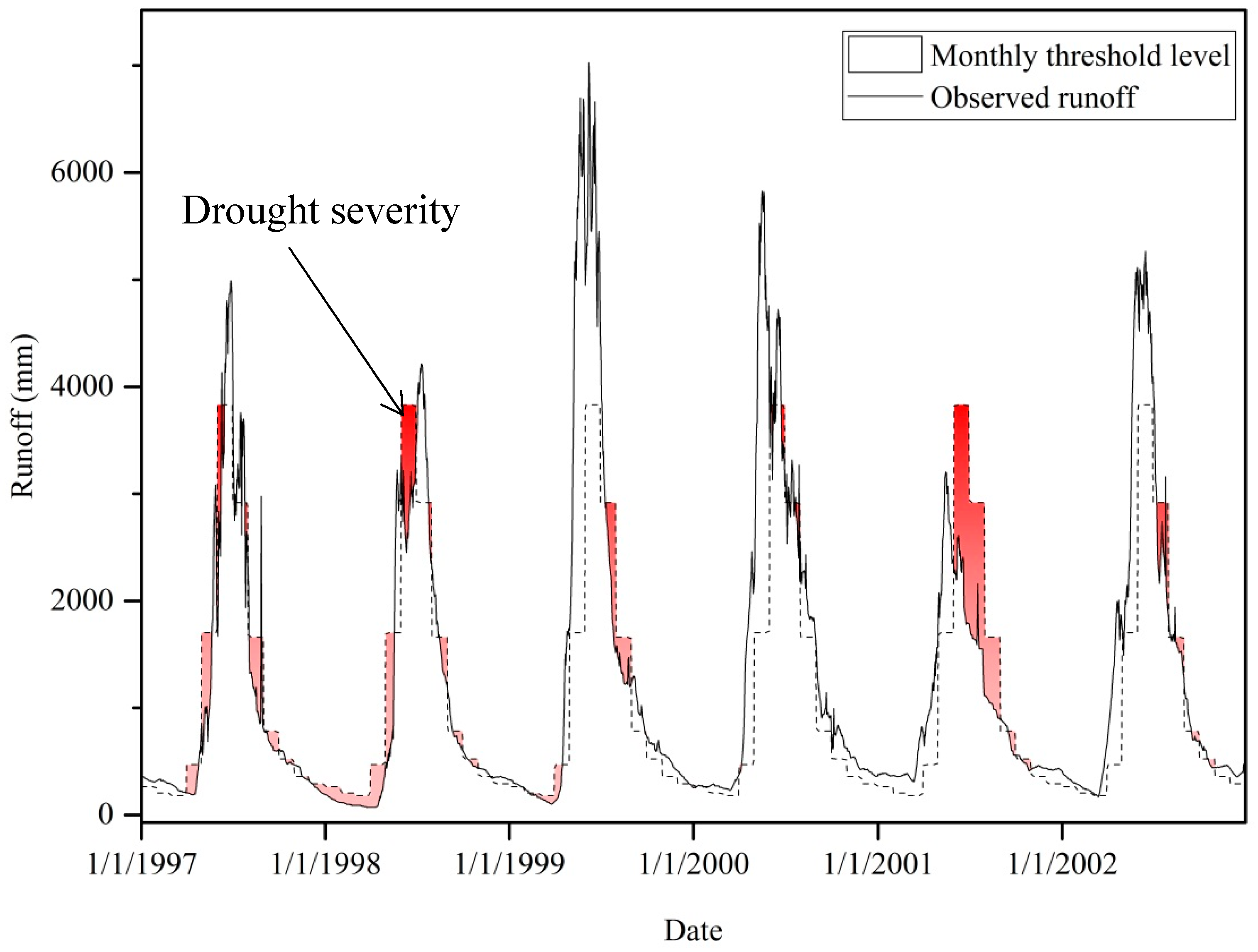
2.5. Development of Threshold Levels for a Hydrological Regime

Developing threshold levels for a hydrological time series is essential for water-resource management in the study region. There are many approaches to defining these thresholds, but a fixed and transient threshold-variable approach based on different time scales is most suitable for identifying drought events in a basin. A sequence of drought events can be estimated using a time series of hydrological variables with fixed and variable threshold levels [14,17]. In this study, we set the threshold to Q80, which was derived from the flow duration curve of the entire study period [17,18]. The discrete monthly threshold values were obtained using a centered moving average of 30 days [17]. Each threshold level event was characterized by its duration, deficit volume and time of occurrence. Figure 5 shows the basic concept of this drought analysis:
TL e ( t , x ) = 1   for   R ( t , x ) R thr ( t , x )
0   for   R ( t , x ) R thr ( t , x )
where TL e ( t , x ) is a threshold event at a given time that is equal to or exceeds the threshold. Drought events were identified based on the length of time over which the threshold was exceeded for two events, and the duration of each event, which were expressed as follows:
d i ( min ) d thr
d i d i 1 d thr
where d i ( min ) is the minimum event duration and d thr is the threshold duration of the event. The minimum event duration (10 days) was considered in this study, as well as the inter-event duration. The total duration of all of the events can be estimated using the following equation:
d tn = i = 1 n TL e ( t , x )
where d tn is the total duration of an event at a given location. The severity of each event was calculated as follows:
S ( t , x ) = R thr   ( t , x ) R   ( t , x )   for   TH e ( t , x ) = 1
where S ( t , x ) is the severity of event i at time t and location x. The total severity of event i is defined as:
S tn = i = 1 n S ( t , x )
where S tn is the cumulative severity of the event and the deviation of the runoff from the threshold.
A sequence of drought events can be identified based on the thresholds of hydrological variables (Figure 6). In the case of a long dry period, long drought events can be divided into various minor drought events. Because these minor drought events are not independent of each other, the authors of [15] described them as pooled events. In the case of pooled events, the severity and maximum severity can be calculated according to [11]:
d pool = d i + d i + 1 +
S pool = S i + S i + 1 +
S max = MAX ( S maxi , S max   i + 1 + )
where i is a hydrological drought event and i + 1 is the following hydrological drought event. We eliminated minor drought events from our analysis by excluding events with durations of less than 10 days, similar to other researchers [23].

2.6. Sensitivity of Hydrological Regime to Climate

The climate sensitivity of runoff can be analyzed by using different models to investigate the different characteristics of the basin, as well as variations in the hydro-meteorological parameters [33,34,35,38,56]. In addition to hydrological and physical models, we used a climate-sensitivity model to evaluate the sensitivity of runoff to climate change. This model is both non-parametric and parametric [19,39,57]. The limitations of this model include that it does not take into account changes in the frequencies and distributions of the hydro-climatic variables; furthermore, it does not include changes in the characteristics of the vegetation under different climatic conditions [26,32,58]. However, in the absence of a more detailed study, the climate elasticity method provides a simple non-parametric estimation of the climate sensitivity of the runoff. The authors of [5,29] derived the following climate-elasticity model to measure the variation in climatic variables according to the runoff of the basin:
ε = dR R dX X = dR dX X Q
where R is the runoff and X is a given climate variable in the basin. Here, we used precipitation and temperature as the climate variables. It is essential to consider the influence of global warming on runoff in the study region. Therefore, we calculated the precipitation and temperature sensitivity based on a non-parametric approach. The climate elasticity is defined by Equation (15), and can be estimated using a non-parametric climate elasticity approach [29]. Based on Equation (15), the climate sensitivity of the runoff can be defined as follows:
R = P ( ε P R P ) + T ( ε T R T )
where P , R , T , are the variations in the mean runoff, precipitation, and temperature, respectively. Recently, the authors of [5] suggested a linear regression coefficient for runoff and climate variables. A similar equation has been used to estimate the sensitivity of runoff to climate variables using multiple regression [40]:
ε X = Median ( R I R ¯ X I X ¯ X ¯ R )
where R is the total runoff, R ¯ is the mean runoff, X is the climate variability, and X ¯ is the mean annual climate variability. The climate sensitivity of the runoff can also be estimated using the least squares method, and it can be modified by taking into account the ratio of metrological and hydrological variables and the correlation between runoff and climate variables, as follows:
ε X = X R ( X i X ¯ ) ( R I R ¯ ) ( X i X ) 2 = γ X , R × ρ X , R × σ R σ X
where γ and ρ are the ratio of metrological and hydrological variables and the correlation coefficients between the climate variables and the runoff, respectively. The estimators defined in this equation are more sensitive to runoff than median base statistics [29,40]. The fraction and correlation coefficients of the climate variables with respect to runoff can be estimated accurately [36].

3. Results and Discussion

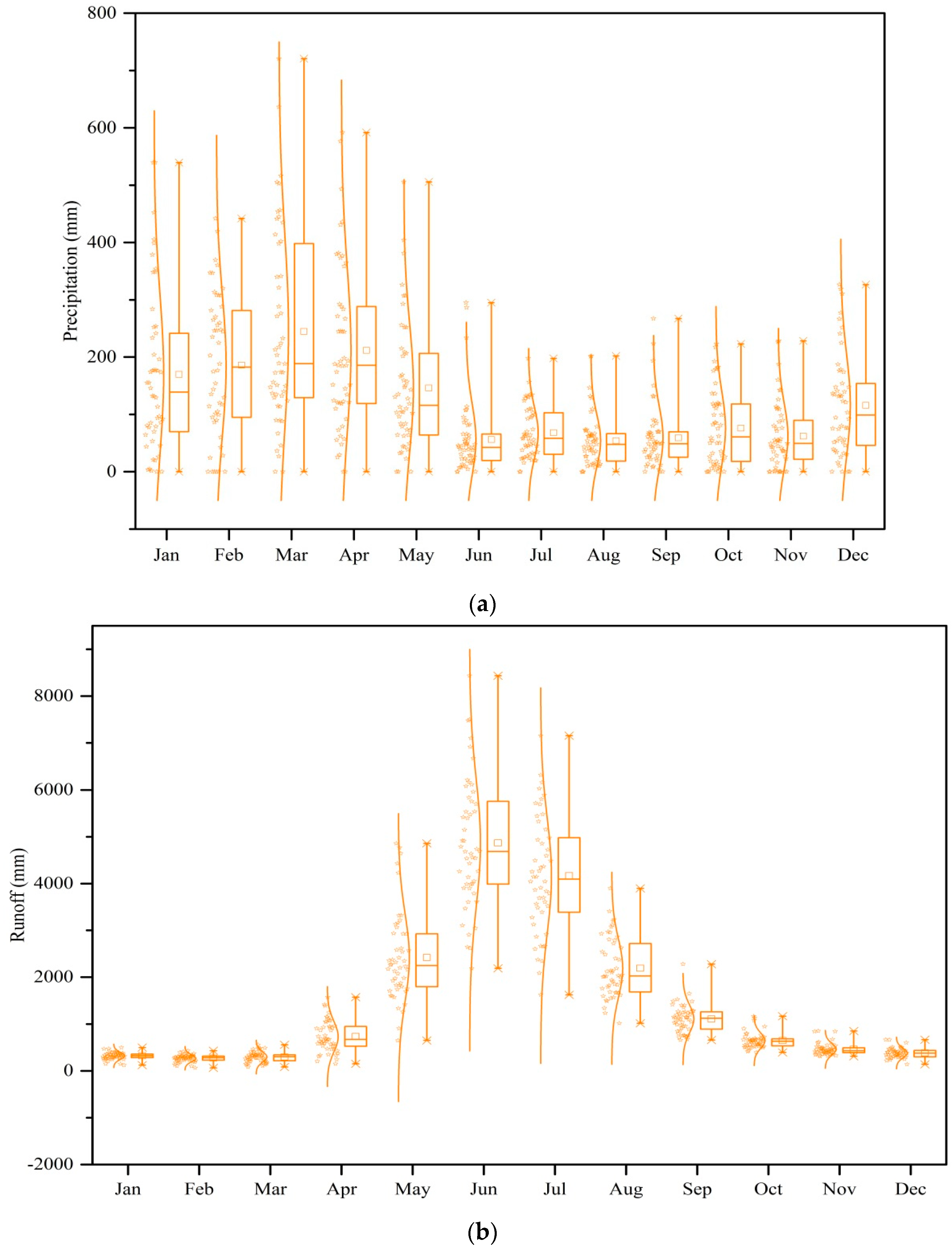
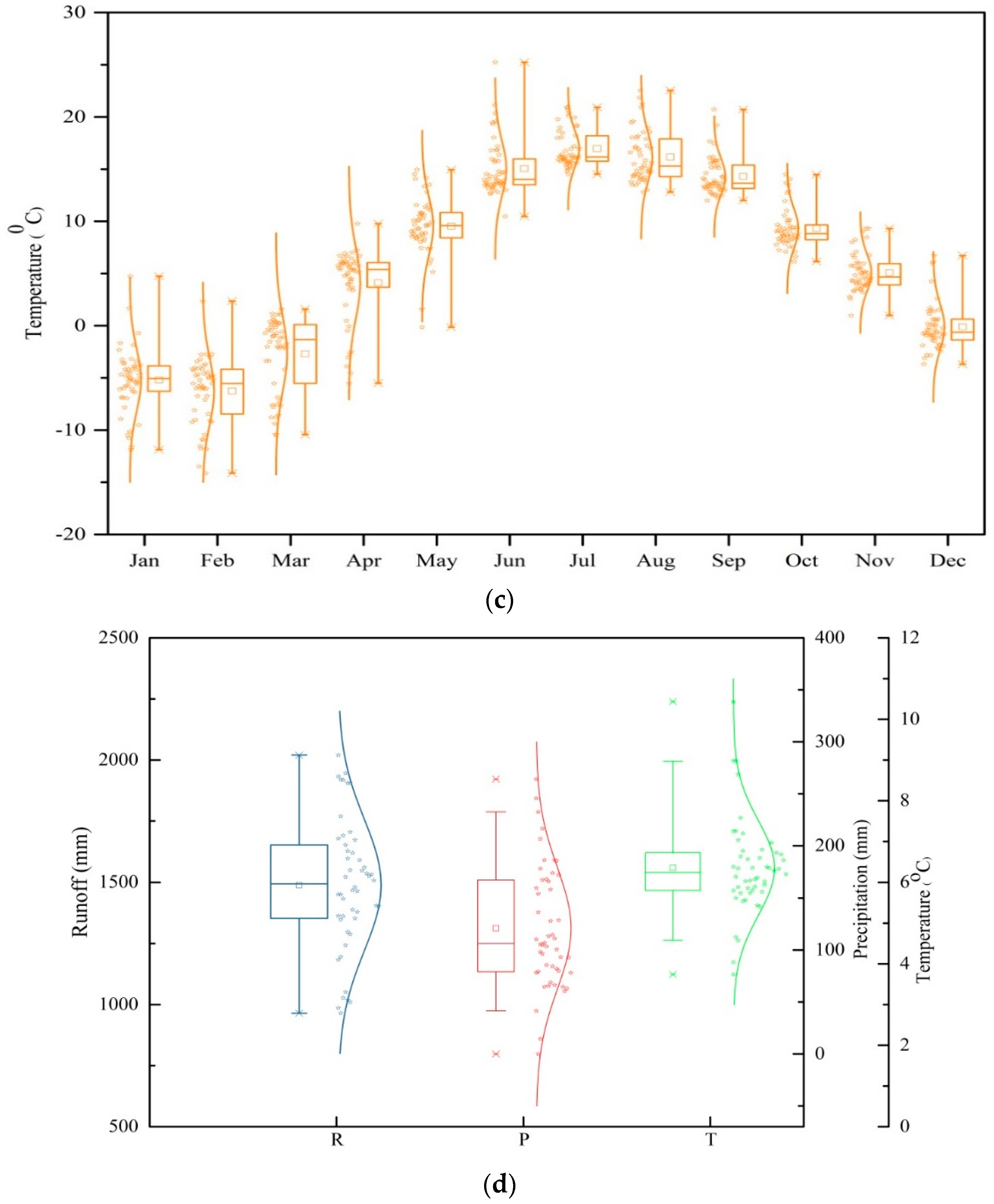
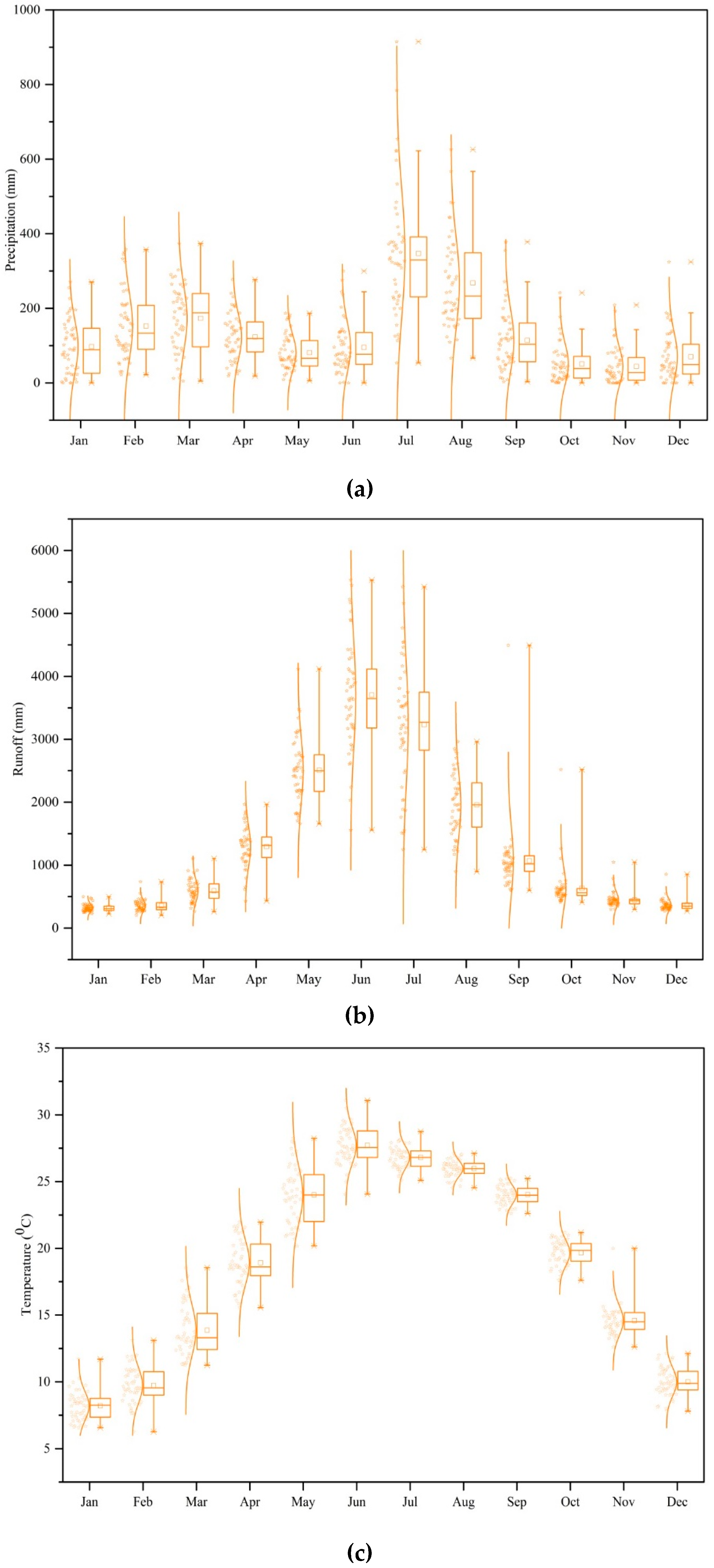
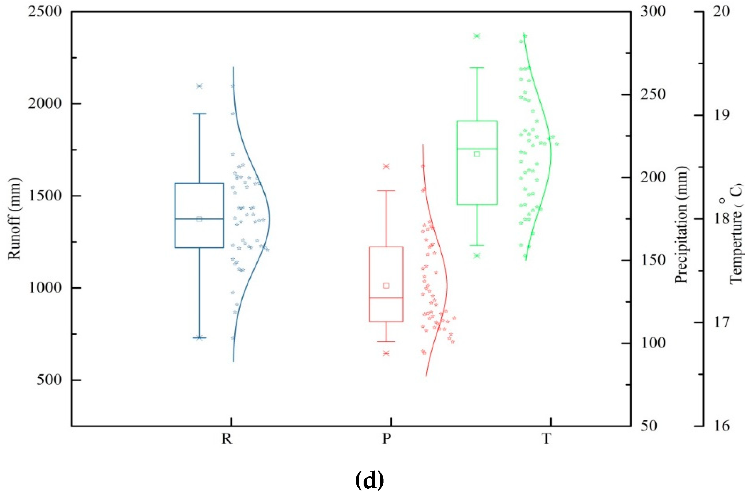
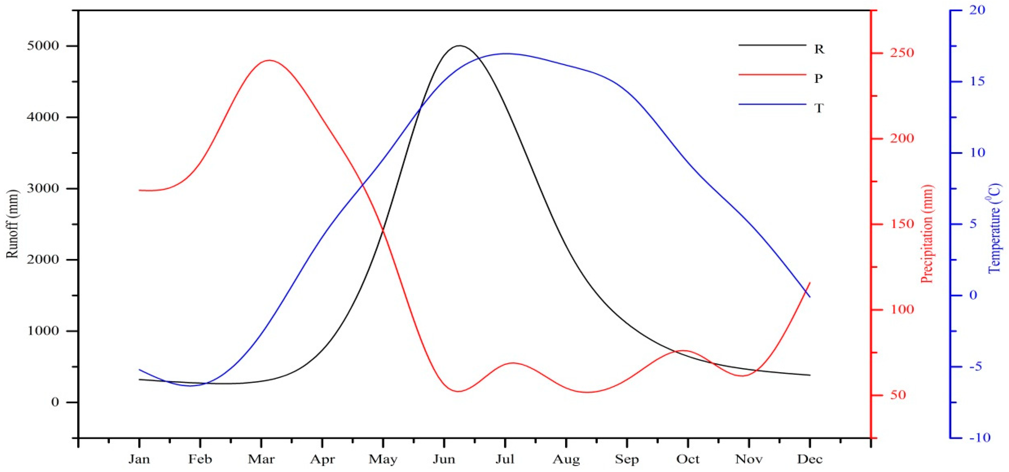
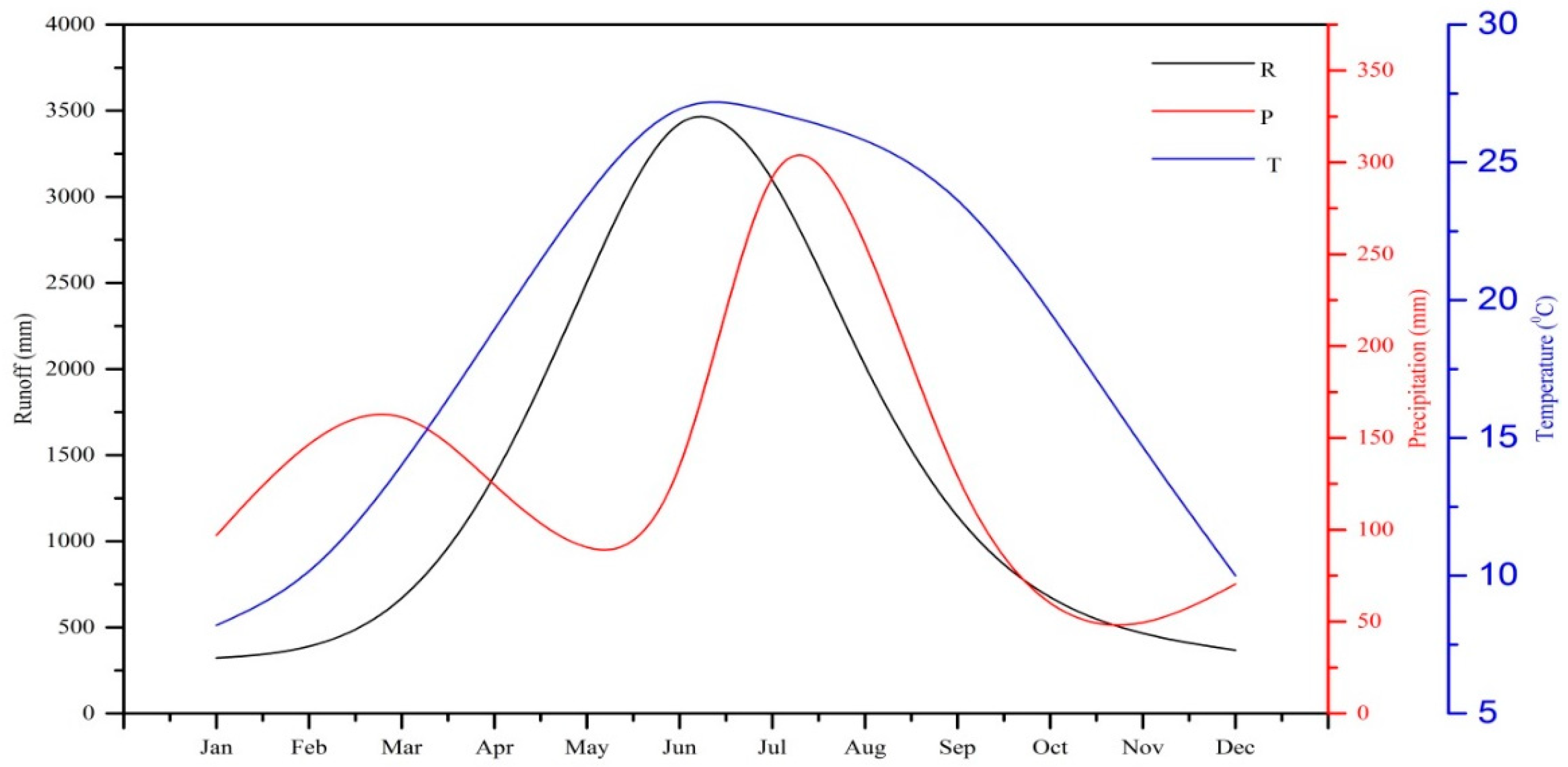
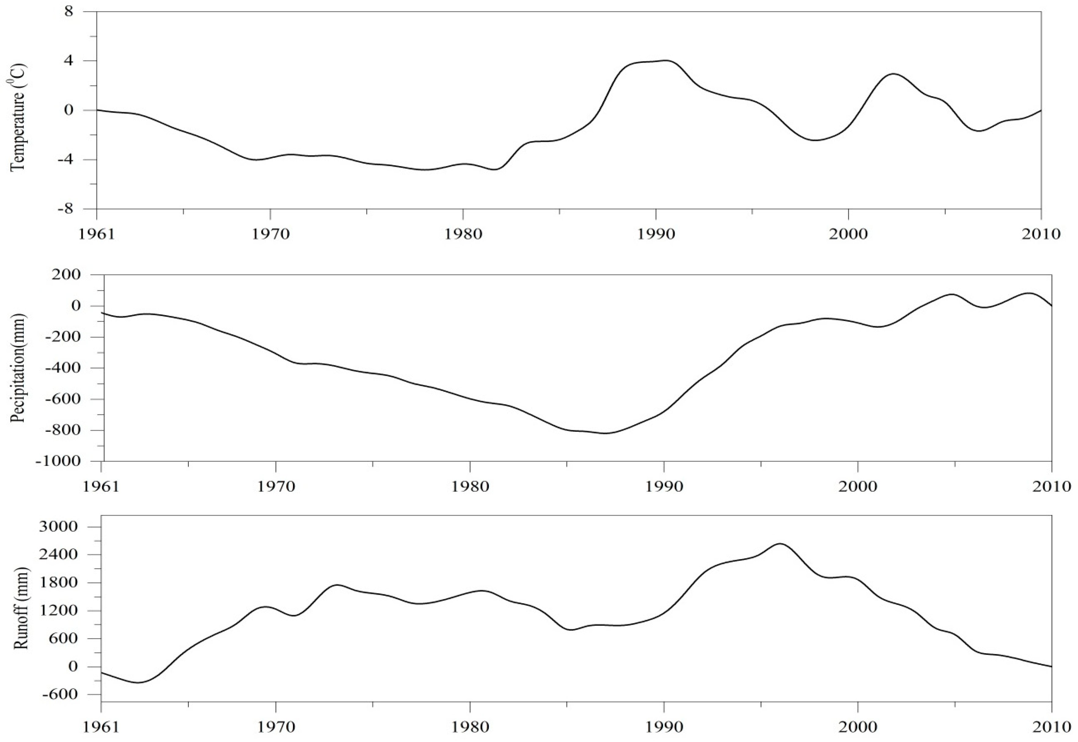
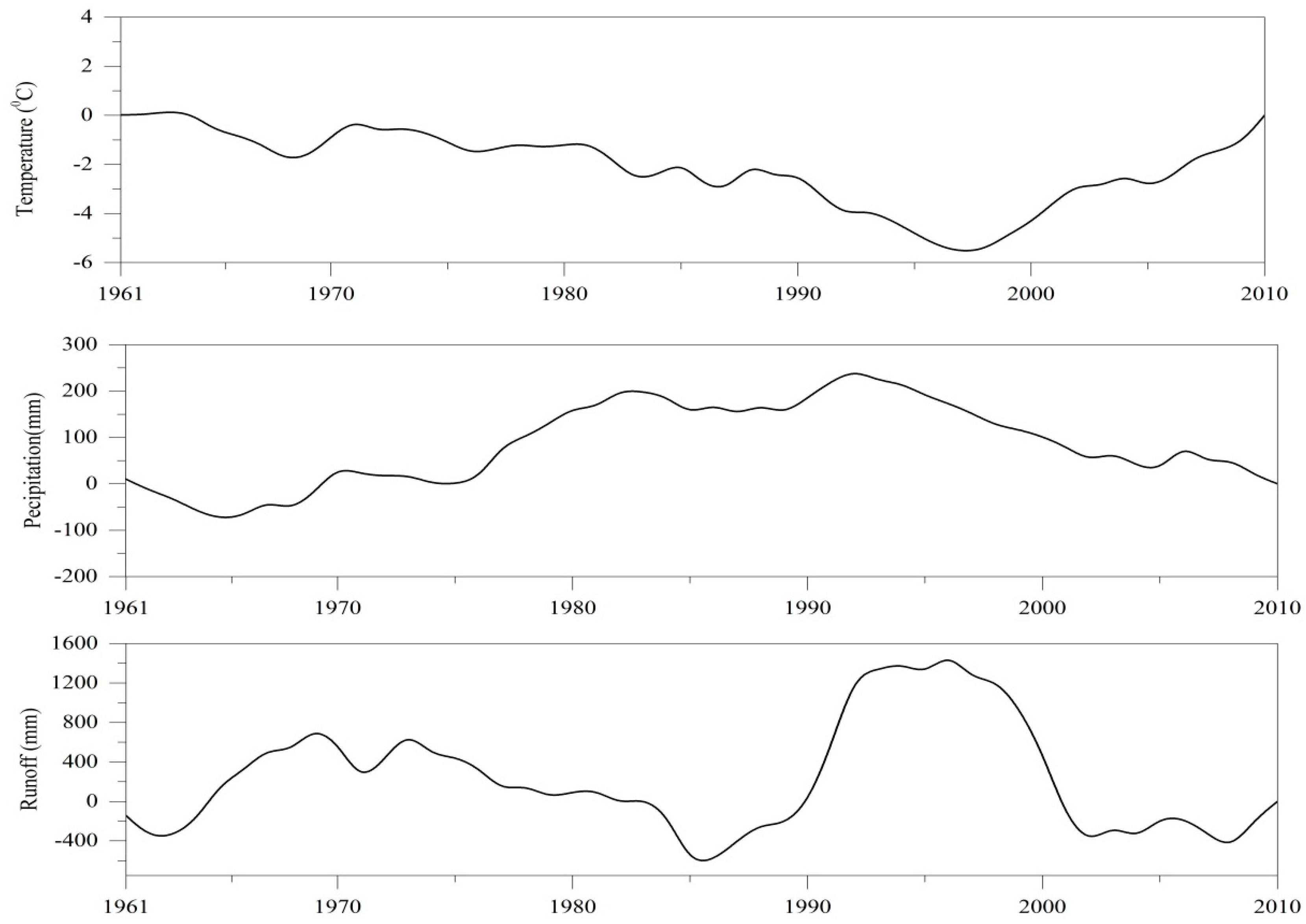
3.1. Spatial and Temporal Characteristics of Precipitation, Temperature and Runoff

We investigated the spatial and temporal characteristics of temperature, precipitation, and runoff in both zones in the study area using the non-parametric MK trend test, Sen’s slope estimator, and graphical ITA with innovative trend statistics. Our results were consistent across all methods, as well as in terms of the innovative statistics, which we used to compare the methods at a practical significance level of 10%. In the case of Zone I, the MK trend was found to be significant for decreasing and increasing runoff in July and November, respectively. These results were consistent with those reported by other researchers [41,42]. We also identified significant temperature trends in April in Zone I. In Zone II, the temperature increased, and precipitation decreased significantly, during December, as shown in Figure 7.
The monthly precipitation of Zone I increased beyond the practical significance level according to the MK test. The annual precipitation also increased according to Sen’s slope estimator, the graphical method, and the modified ITA statistics. Almost all of the statistical approaches indicated an increase in the temperatures of the zones over the study period, except in January, February and March. However, almost all of the monthly and annual runoff values decreased, except those for September, October, and November. Overall, the annual runoff trend decreased consistently in all approaches. The annual precipitation of Zone II decreased according to the graphical result, and the modified ITA approach and Sen’s slope estimator indicated a significant decreasing trend. The annual temperature increased and, according to the graphical method and the modified ITA, the runoff increased (see Figure 8). Significant variation in precipitation in December was identified by the modified ITA statistics but not by Sen’s slope estimator or the graphical method. The authors of [44] reported similar trends in precipitation, temperature and runoff in this region.
Table 2 and Table 3 compare the trends in results among Sen’s slope estimator, the graphical method, and the modified ITA statistics for the two zones. The bold text indicates the practically significant trends during the study period. The modified ITA statistics estimated more significant trends in precipitation at the practical significance level than the other non-parametric methods, i.e., the MK test and Sen’s estimators. The modified ITA statistics support the results obtained by the other methods. However, many trends in Table 3 identified by the modified ITA statistics were not identified by the other methods. Such inconsistencies in the results can be seen in both the monthly time series and the graphical data (Figure 9). The other methods are less efficient at detecting significant trends, which play a key practical role in water management.

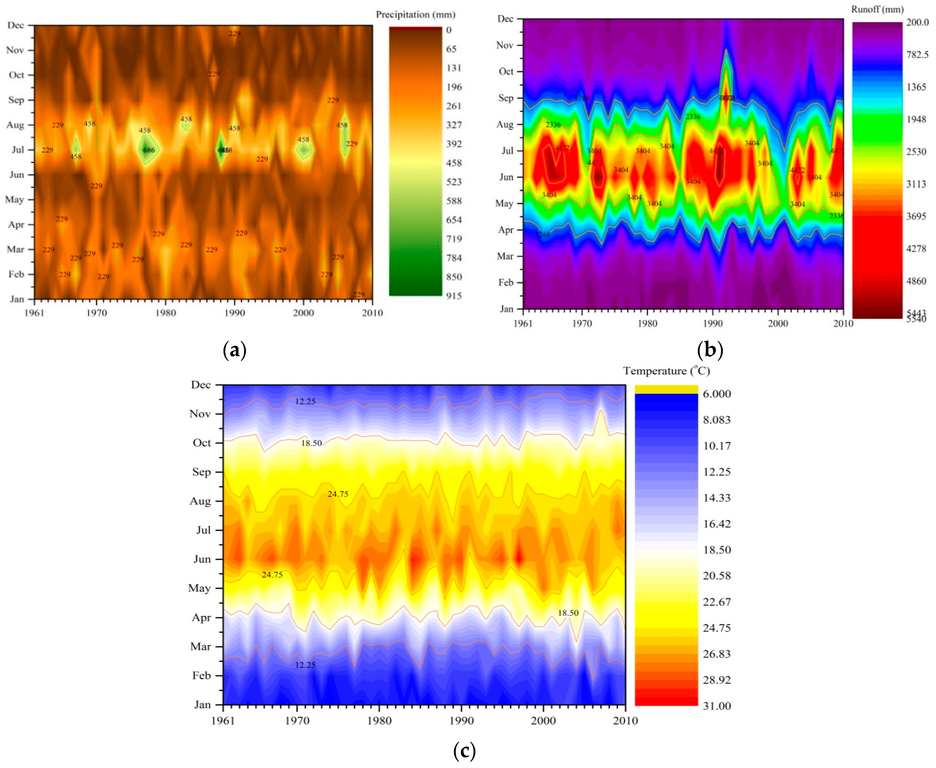
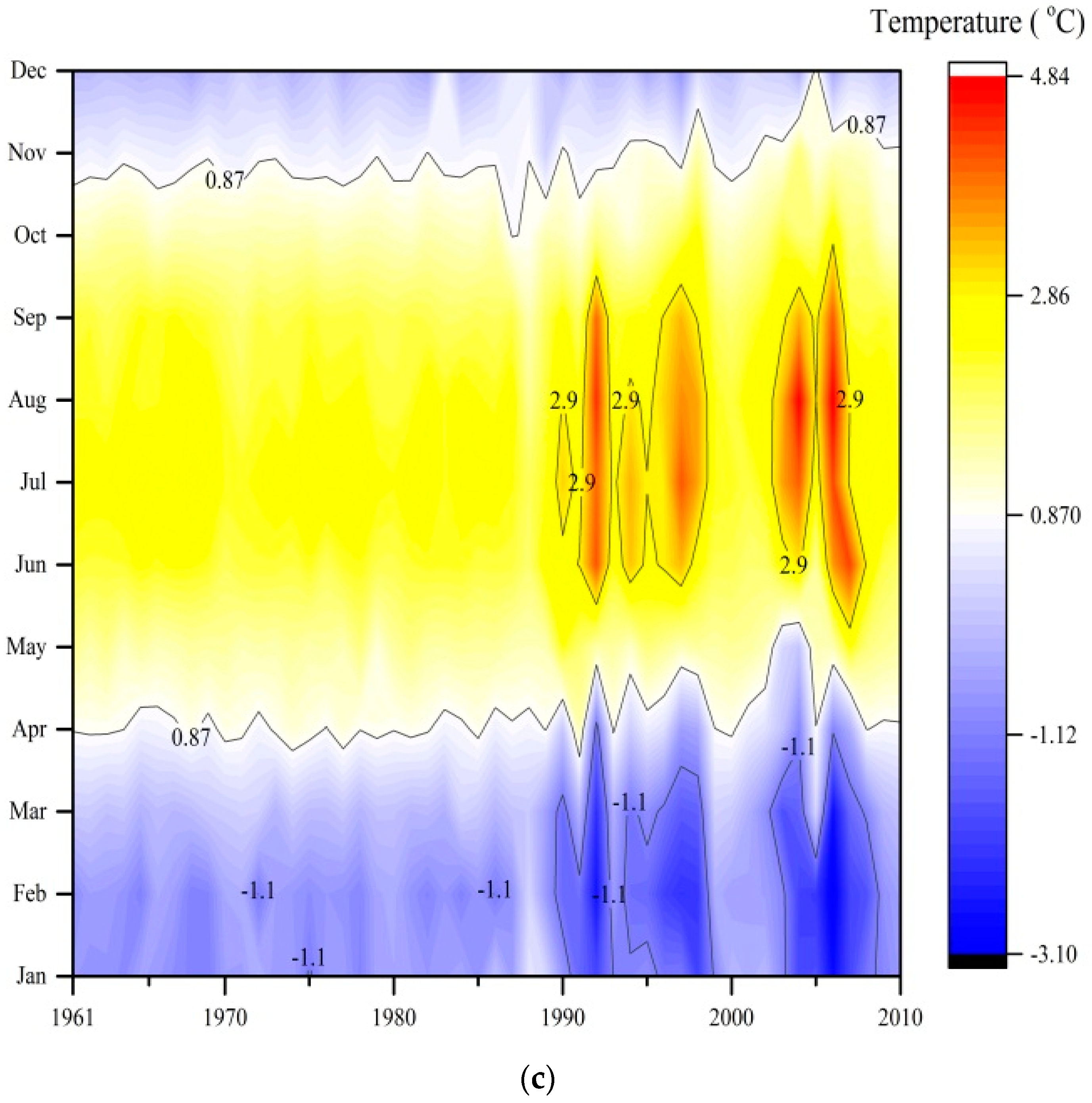
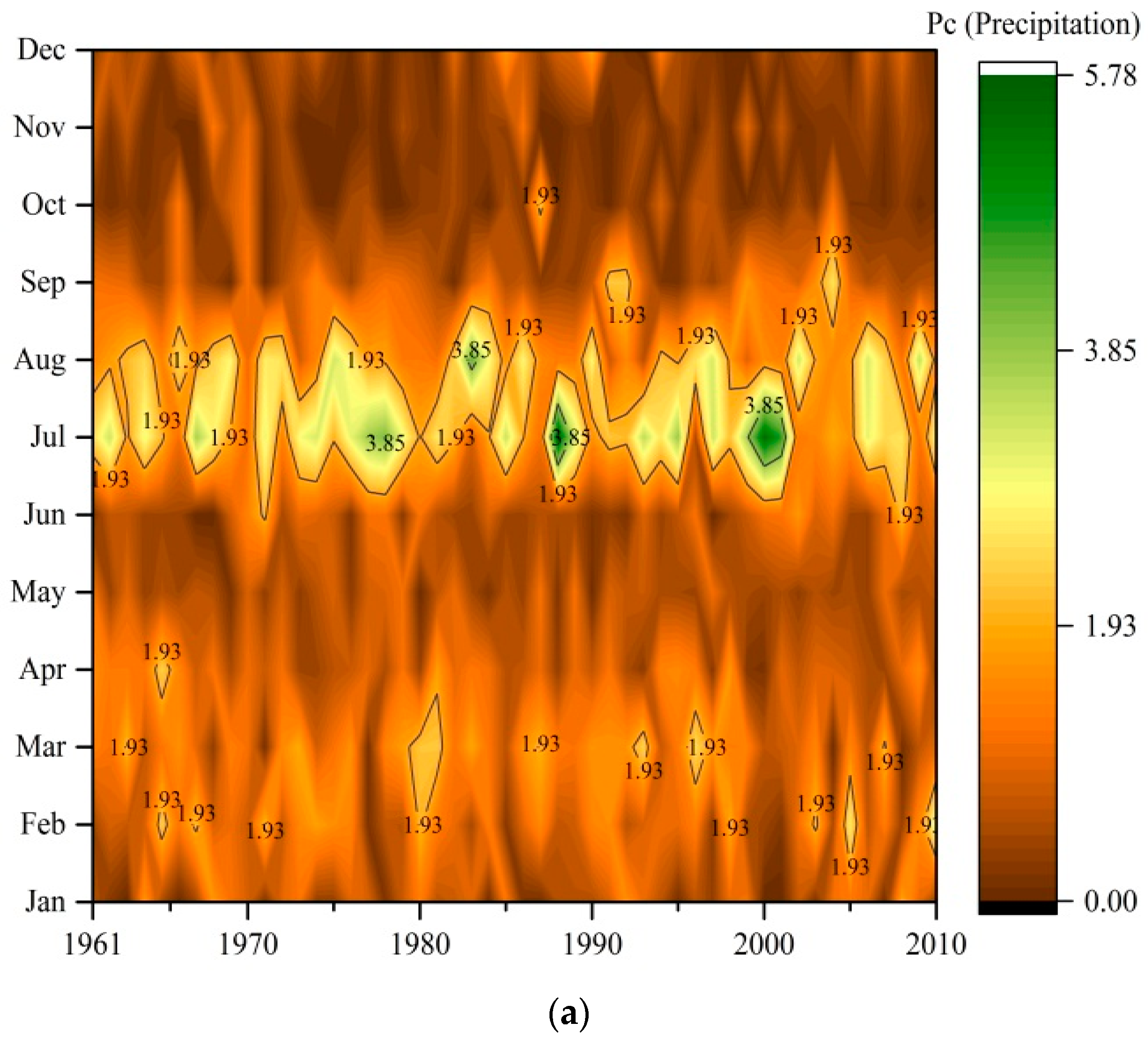
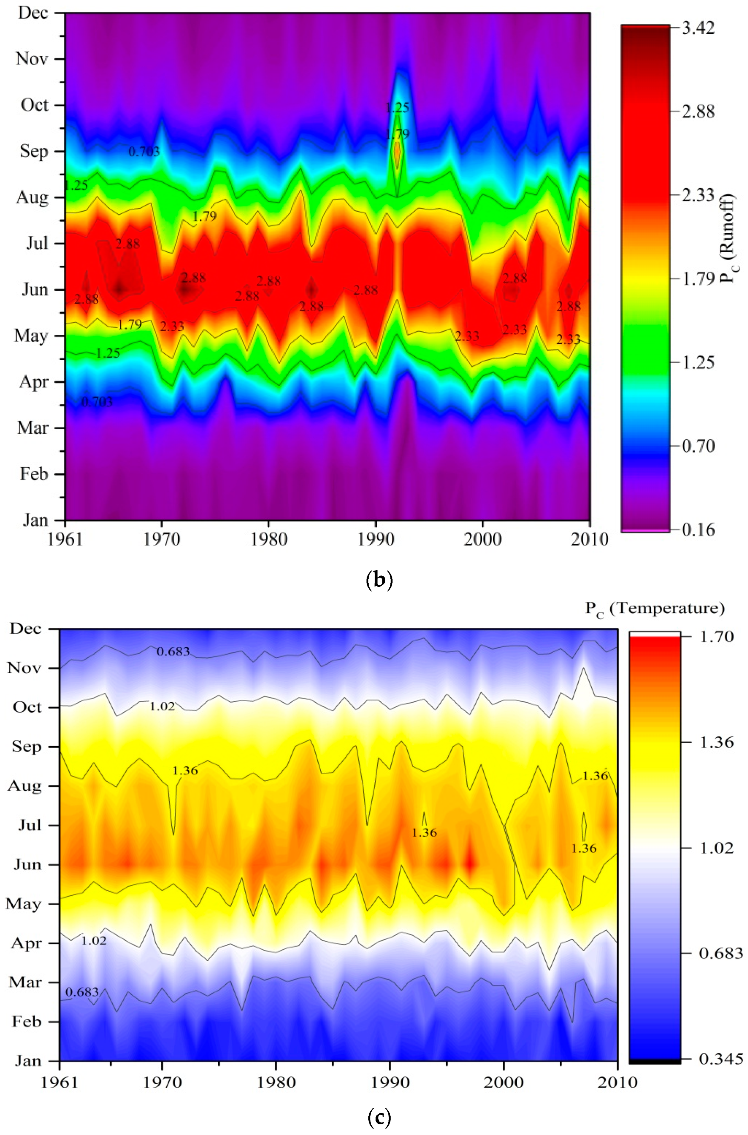
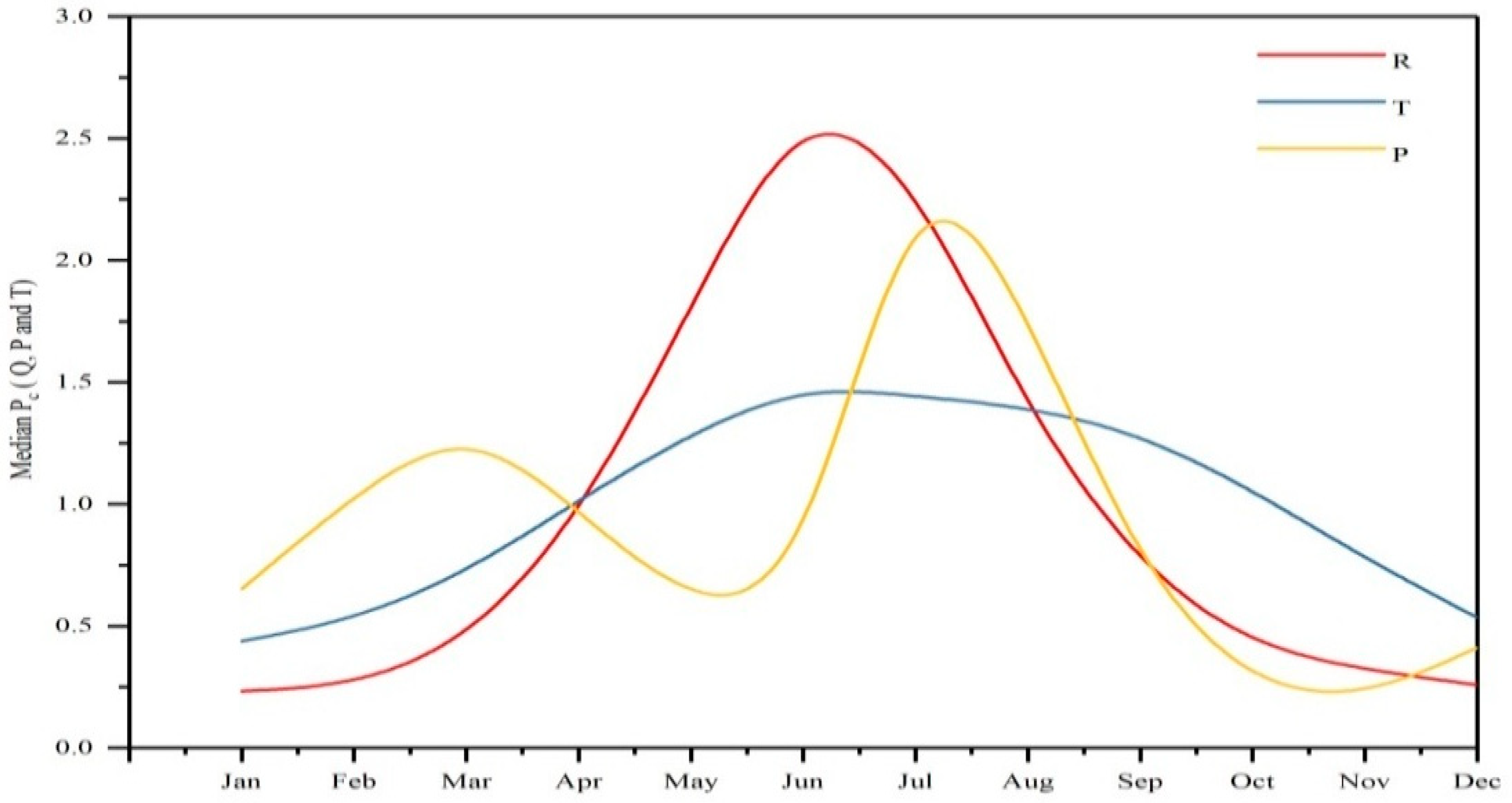
3.2. Iso-Plots of Precipitation, Temperature and Runoff

We represented the time-series data as a two-dimensional (2D) matrix (month × year). The matrix created in origin software. Then, the dimension of the matrix was set as 12 (month) by 50 (year) according to the available time period. The matrix was then transformed into an image and an appropriate color scheme was used to display the data. We enhanced the image for small data samples by applying interpolation methods (linear, quadratic, logarithmic, etc.) to each data point (or pixel) based on the values of the surrounding data points. Then, iso-plots of specific parameters were drawn for specific interval to identify the pattern of hydrological regime. Then, legends of the image were inserted on the iso-plots. We can identify both events and their relationships to precipitation and temperature in the iso-plot.
Changes in precipitation, temperature, and runoff indicate significant changes in the hydrological regimes of the Kunhar River basin. We generated iso-plots of the runoff, temperature, and precipitation so that we could visualize the climate sensitivity of the hydrological regime of different zones of the Kunhar River, as shown in Figure 10. According to the isographs, precipitation and runoff occurred during specific months in the study period, and temperature played a vital role in determining the peak runoff. The runoff of Zone I was highest in July (5419 mm) of 2003, but the July runoff decreased over the last decade compared to 1990–2000. This reduction in runoff was due to the increase in the duration of high-temperature periods. The precipitation in this region also decreased in February, March, and April. The rise in temperature and reduction in precipitation reduced the runoff over this period.
The reduction in snowfall also reduced the availability of water in this zone. Extreme July runoffs are clearly identifiable in the isographs for the years 1966, 1973, and 1996. The maximum precipitation occurred in March 1996, which was the same year as the maximum temperature, which was observed in July (18.20 °C). We analyzed the inter-annual variability in temperature, which was clearly visible in 1966, 1973, and 1996. The variations in the temperature, precipitation, and runoff are shown in Figure 11, in which it can clearly be seen that these variables are inter-related. The iso-plots for the temperature of Zone I show that the duration of the period, during which the temperature was highest, increased after 2000. The minimum July runoff occurred in 2001, whereas the maximum July temperature occurred in 2000. The maximum temperature was always greater than 15 °C between 2000 and 2010, whereas the minimum July temperature occurred in 1972 (14 °C). The year with the most precipitation was 1963, when the maximum precipitation was 720 mm in Zone I.
In Zone II, the maximum runoff occurred during the month of July, as shown in Figure 12 and Figure 13. July also had the highest temperature and runoff, because runoff follows 1 month after precipitation. It appears that precipitation does not directly affect the hydrological regime of Zone II. The regime can be categorized in terms of the coupling between the precipitation and increasing temperature, which influences the hydrological process in Zone II. The highest runoff was observed in July 1991 (5530 mm). Similarly, the maximum precipitation (914 mm) occurred in the same month of 1988. From the isographs, the durations of the periods with high temperatures increased after 2000.
The precipitation isograph shows the decrease in precipitation over this period. The minimum runoff occurred in July 2001 (533 mm), when the temperature was 27 °C in Zone II. The decrease in runoff from 2000 onwards should be investigated in terms of its effect on the hydrological regimes of the two zones. The effects of variations in temperature and precipitation on runoff should also be taken into account, as mentioned in the previous section detailing our sensitivity analysis. It is also possible to identify different low-runoff events from the isographs. We discuss these in the section on drought analysis. The complexity of the runoff process must be understood so that we can elucidate the mechanisms governing the hydrological regime.

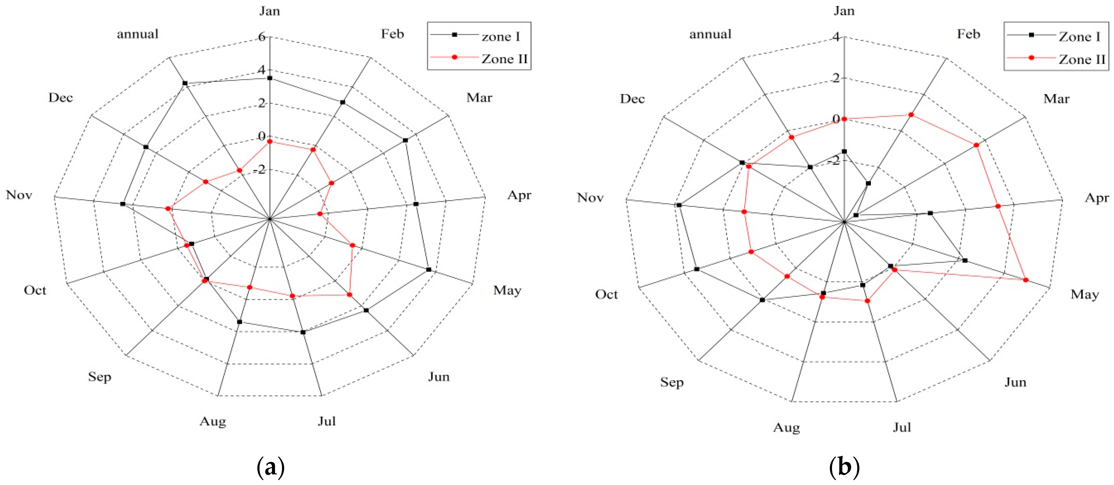
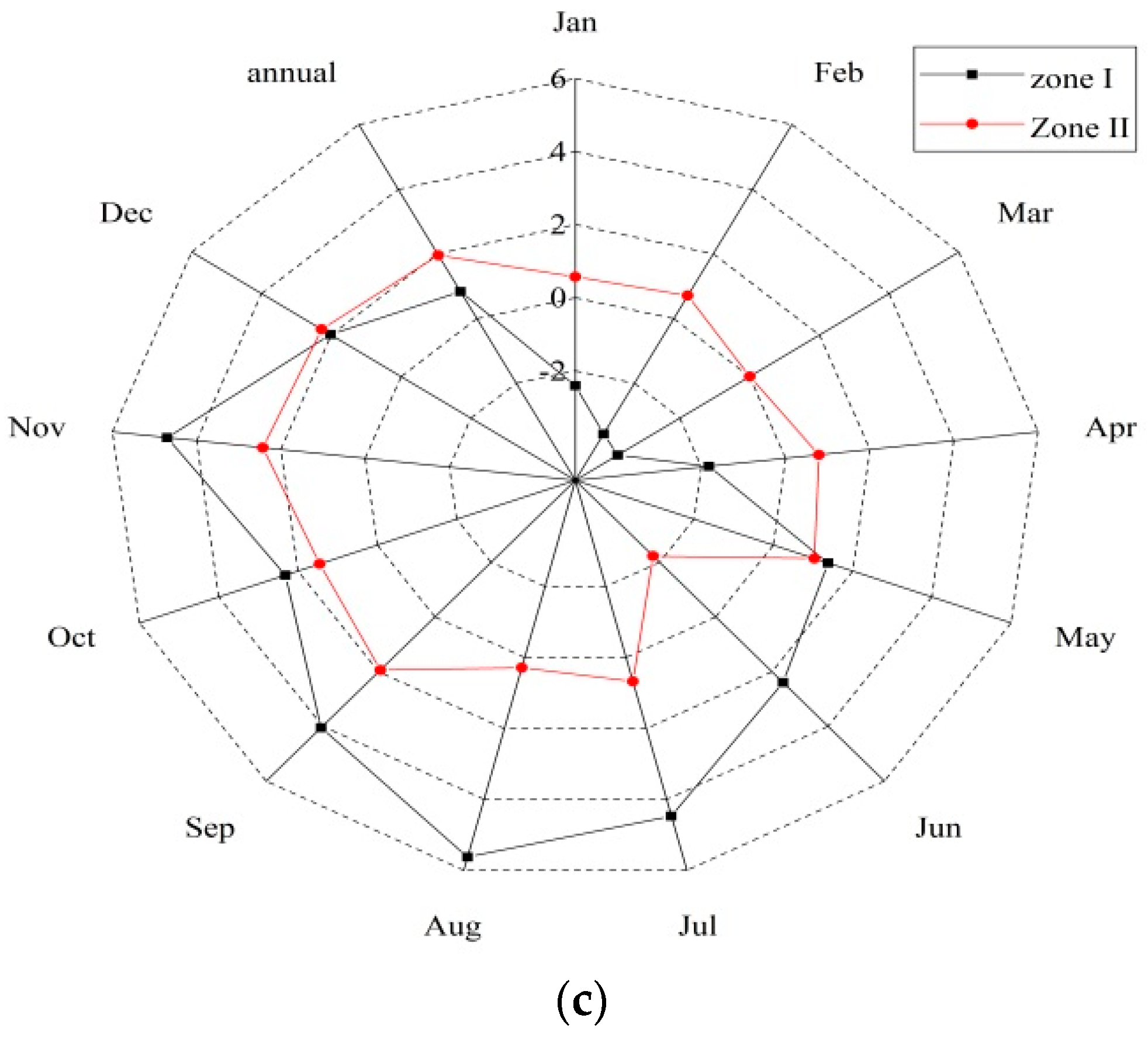
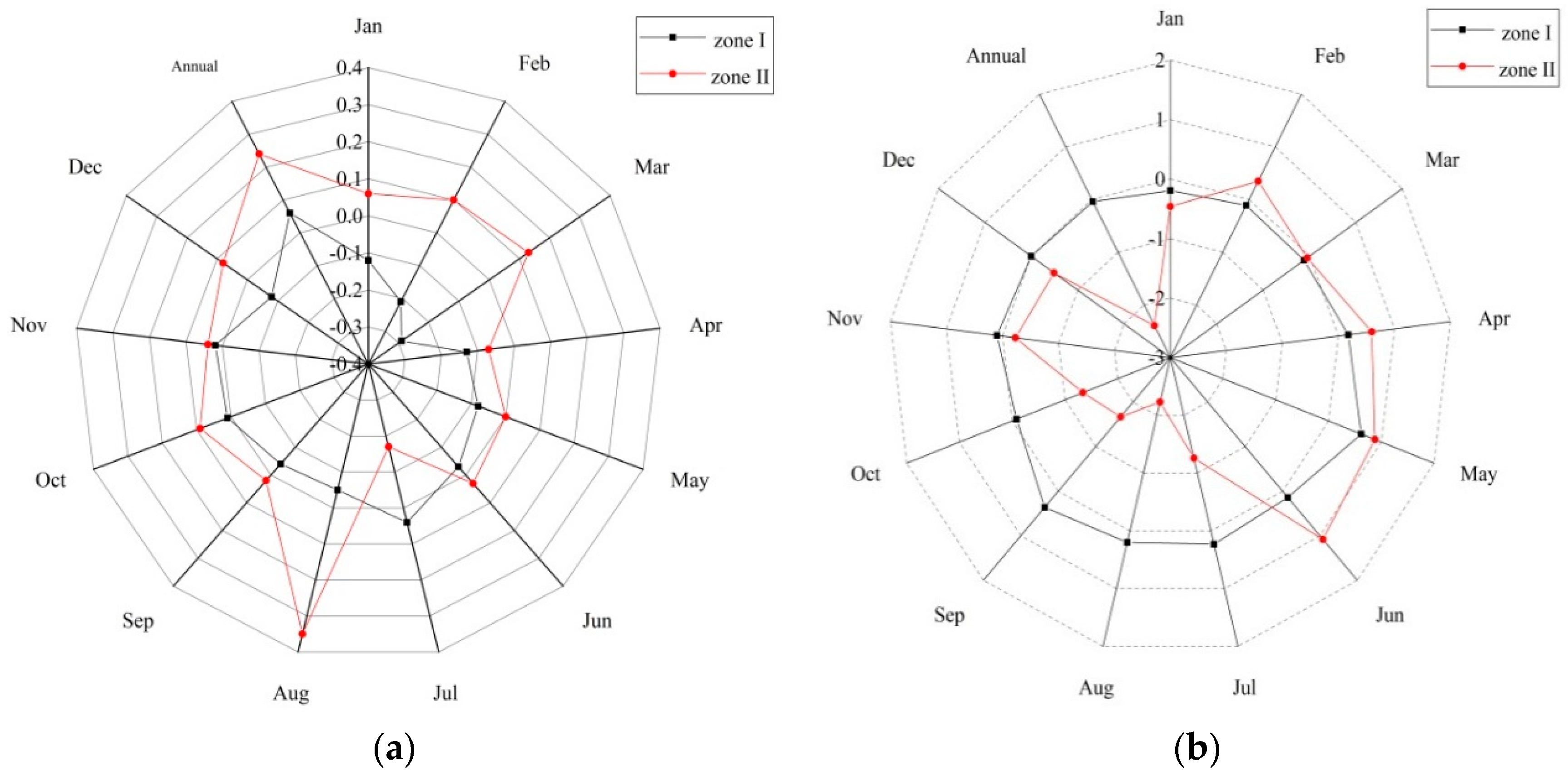
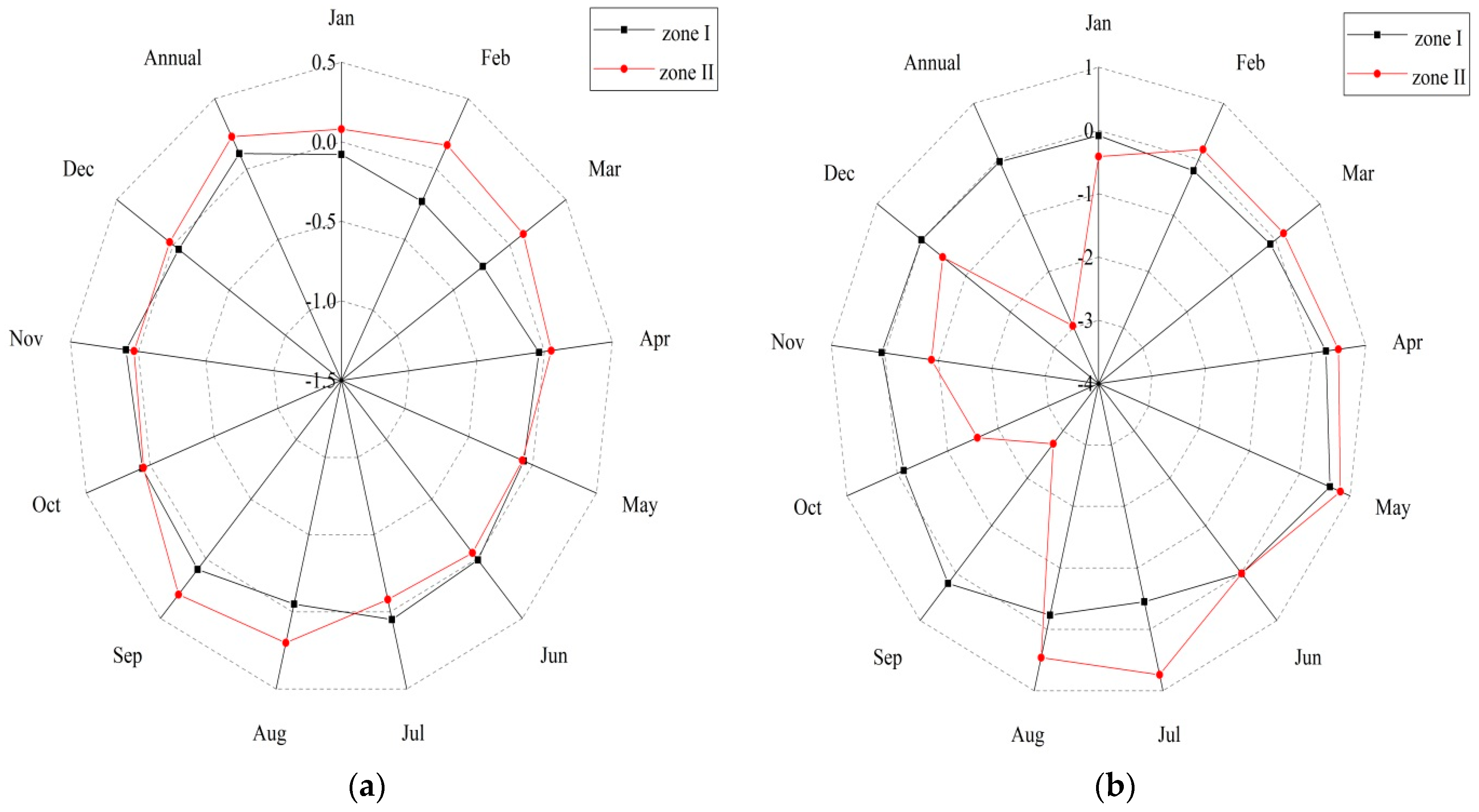
3.3. Hydrological-Regime Variability

Figure 14 shows that the maximum Pardé coefficient of the runoff in Zone I occurred in the months between May and August, whereas the minimum value occurred between December and March. The maximum precipitation occurred from January to March, and the temperature was highest during the period from May to September. The Zone I regime is clearly shown in the contour plots, from which we identified the snow-dominated region of the Kunhar River basin. The regime of Zone I can be considered in the context of different hydrological events, which we have mentioned in the section on drought analysis. Based on the Pardé coefficients, we determined that the maximum median of the runoff occurred in July (2.88), and the minimum median, which was 94% lower than the maximum, occurred in February (0.18). The snow-melting seasons are clearly indicated by the temperature contour plots in each zone.
The Pardé coefficients were significantly higher in 2000 onwards than in previous years. The duration of the maximum Pardé coefficient also increased, which is an indicator of global warming. The minimum Pardé coefficient was lower, and the maximum Pardé coefficient was higher, after 2000 than in early 2000. The maximum values occurred during the months of May, June and July, while the minimum values occurred in the months of December, January, and February.
There were significant variations in the amplitudes of the Pardé coefficients of precipitation and runoff with respect to the temperature of Zone I. The maximum amplitude of the runoff occurred in June (3.55), while the minimum occurred in January, as shown in Table 4. The correlation coefficient between temperature and runoff was −0.18, and that between precipitation and runoff was −0.44. Hence, there was a stronger relationship between temperature and runoff. In Zone I, temperature plays a vital role in the production of runoff by melting snow. The findings of this study are similar to those reported by researchers who have studied other regions, such as the Aggtelek Mountains in Hungary (Pc = 0–5) [59], the Rhine basin (Pc = −0.006–0.004 over various months), and Wurzburg (Pc = 0.4–1.8) [27].
Similar to the case in Zone II, the maximum runoff occurred in the months between May and August, and the minimum runoff occurred in January. The variation between the maximum and minimum values of PCR was 91%. The Pardé coefficient of precipitation peaked in July, when it was 92% larger than its minimum value, and in June, when it was 70% larger than its minimum value. The amplitude of runoff was 87% higher in July than in January, when it was at its minimum. The amplitude of precipitation varied between its maximum and minimum values during the months of July and May (Figure 15).
The contour plot of the Pardé coefficients of precipitation, runoff, and temperature clearly indicate that the runoff depended on precipitation and temperature, but the temperature was found to be the more dominant factor. The maximum amplitudes of precipitation, runoff, and temperature occurred in the months of June, July, and May. These Pardé coefficients did not vary significantly. The variation in amplitudes of temperature, precipitation, and runoff were significant at the 95% confidence level, and the relationship between precipitation and the amplitude of runoff was stronger than that between temperature and the amplitude of runoff, as reported previously by researchers in western Switzerland (Pc 0.2–2.0) [10] and Central Asia i.e., the Zerafshan River basin (Pc = 0–3) [60]. We also evaluated the correlation between the amplitude of precipitation runoff (0.44) and temperature (0.84) and found that the relationship between runoff and temperature was stronger in Zone II.
The runoff peaks in Zones I and II occurred in the same month (July) but the maximum precipitation amounts occurred in different months: March and July, respectively. Similarly, the highest temperatures in Zones I and II were observed in July and June, respectively. Therefore, our sensitivity analysis accurately described the climate sensitivity of the hydrological regime. A closer look at Figure 16 and Figure 17 shows that, compared to Zone II, the runoff lagged 1 month behind the temperature in Zone I. In Zone II, the runoff lagged 1 month behind precipitation, but in Zone I, the Pardé coefficient was highest in March, as shown in Figure 15. The Pardé coefficients behaved similarly in the two zones between February and March, but their behavior varied in the remaining months of the year. The difference between the zones was clearly evident based on the amplitude comparison, which is summarized in Table 4. The variability of the hydrological regime indicated the complexity of the relationship between precipitation, temperature, and runoff, as shown in Figure 18 and Figure 19. The advanced delta change was used to understand the sensitivity of runoff to precipitation and temperature [54,55]. Similar results have been reported by other researchers [28].

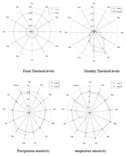
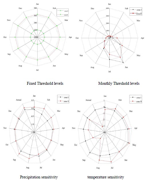
3.4. Threshold Levels of the Kunhar River

We derived two threshold levels, namely fixed and transient variable threshold levels, for runoff. The fixed threshold level was derived from the daily flow duration curve when the probability exceeded 80%, which was used to analyze 50 years of daily runoff data. The monthly threshold was derived for 12 months at Q80 based on the monthly flow duration curves, which were also derived from 50 years of daily data. These two threshold levels are shown in Figure 20. The transient variable threshold levels fluctuated among months due to the natural fluctuations during the low- and high-flow seasons throughout the year [22]. The fixed threshold level was higher for Zone II (12%) than for Zone I, due to the contribution of snow melt to runoff in the area. During the months of January and February, the transient variable threshold was lower than the fixed threshold in both zones. During the period from November to March, the transient threshold level was higher for Zone II than for Zone I. Similarly, the threshold was higher for Zone I than for Zone II in June, July, and August, indicating that snow dominated the runoff in this basin.

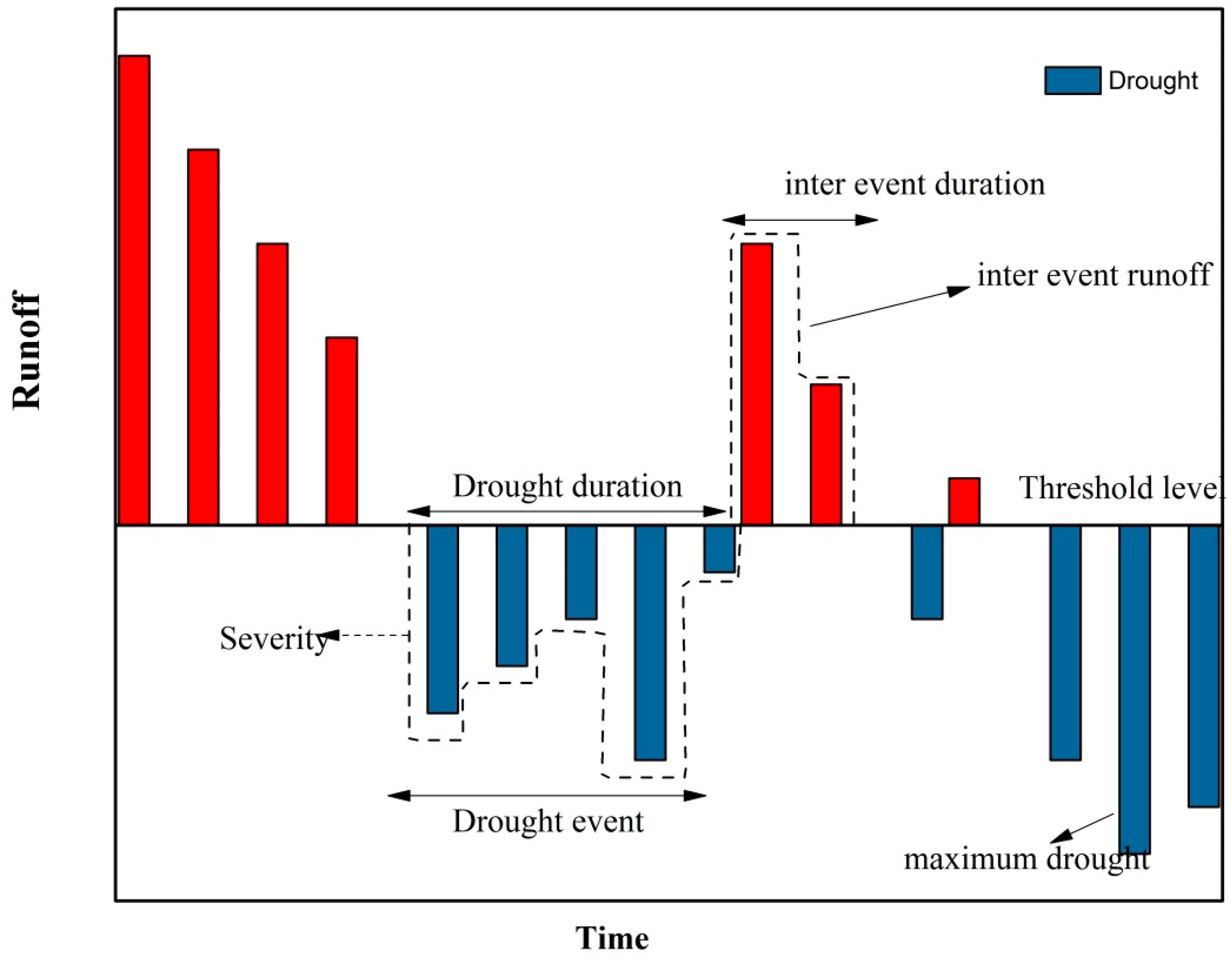
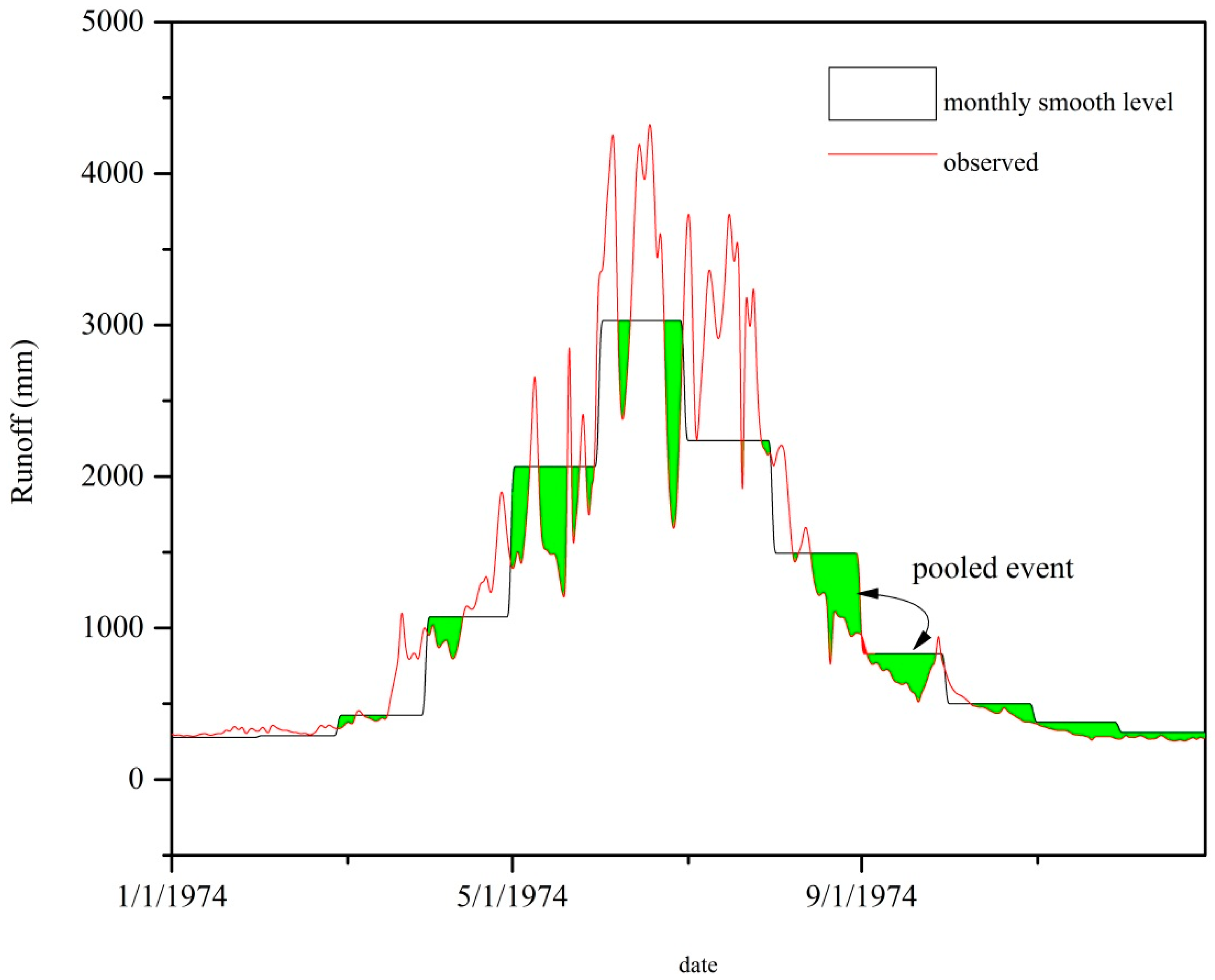
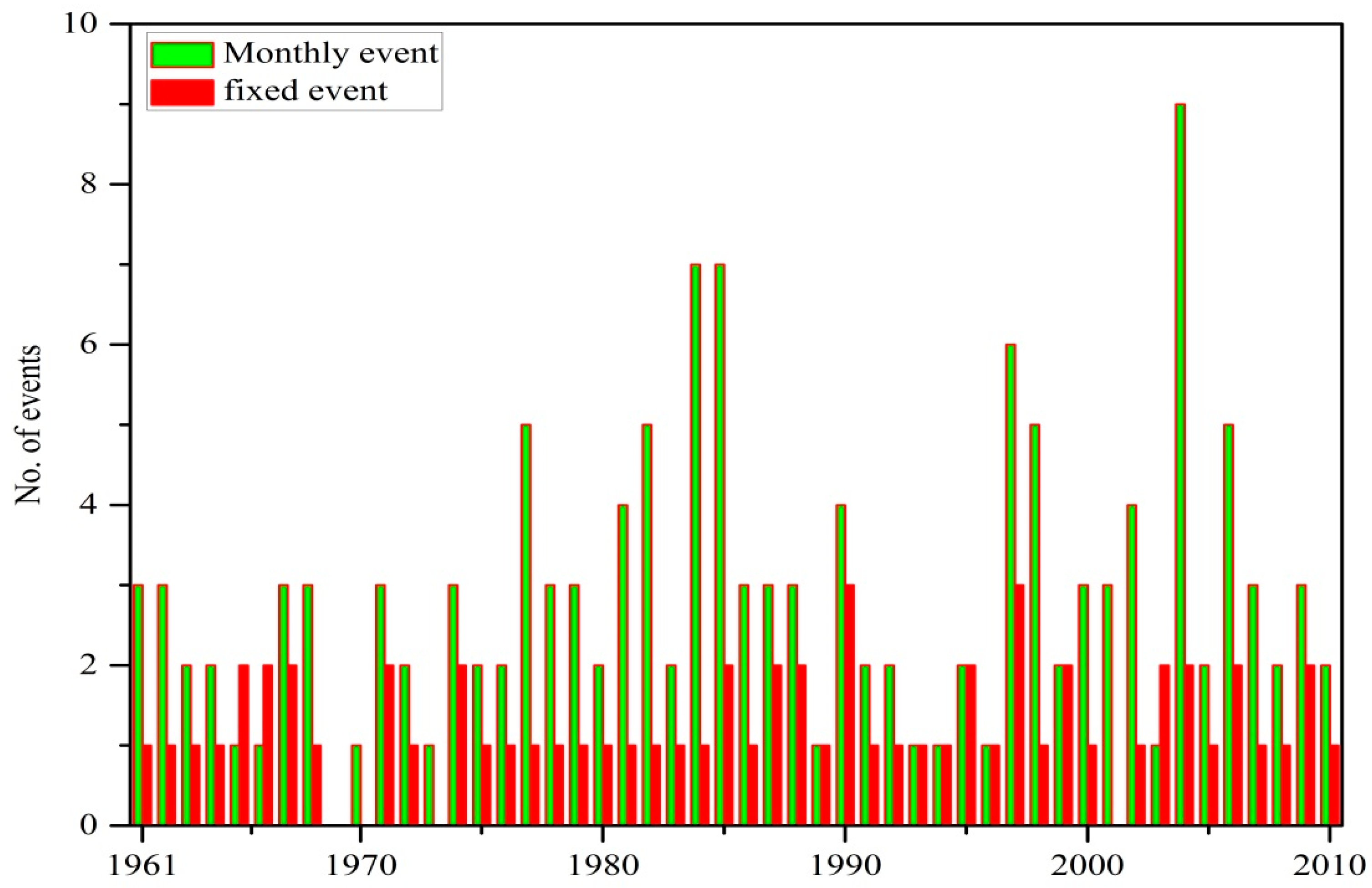
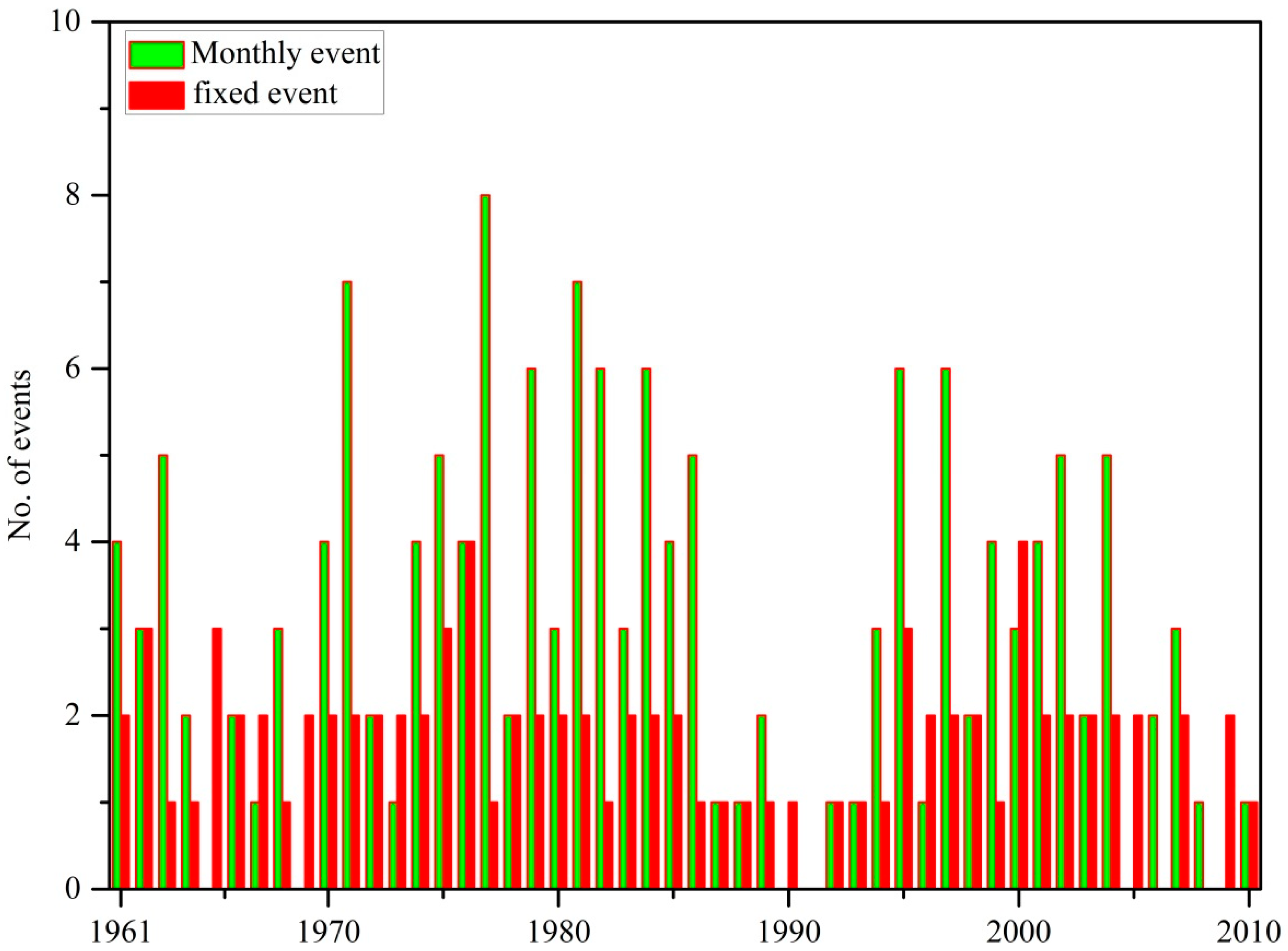
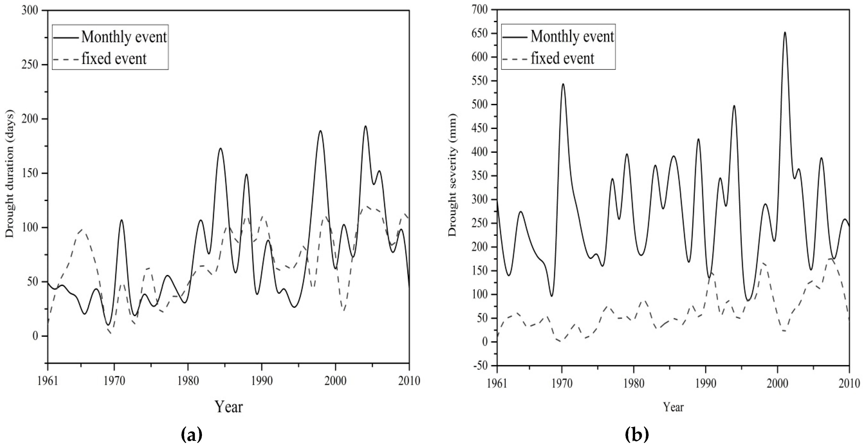
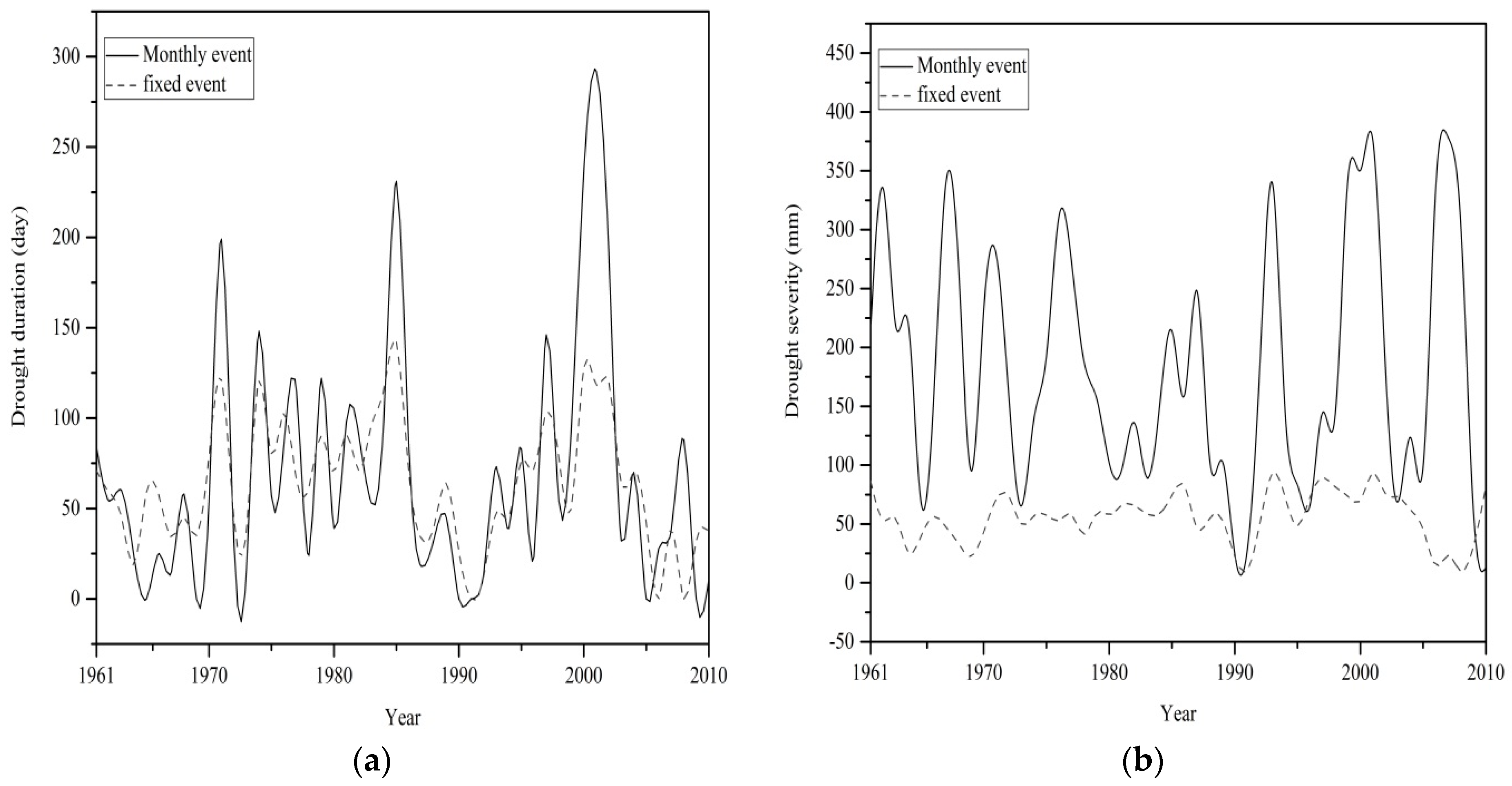
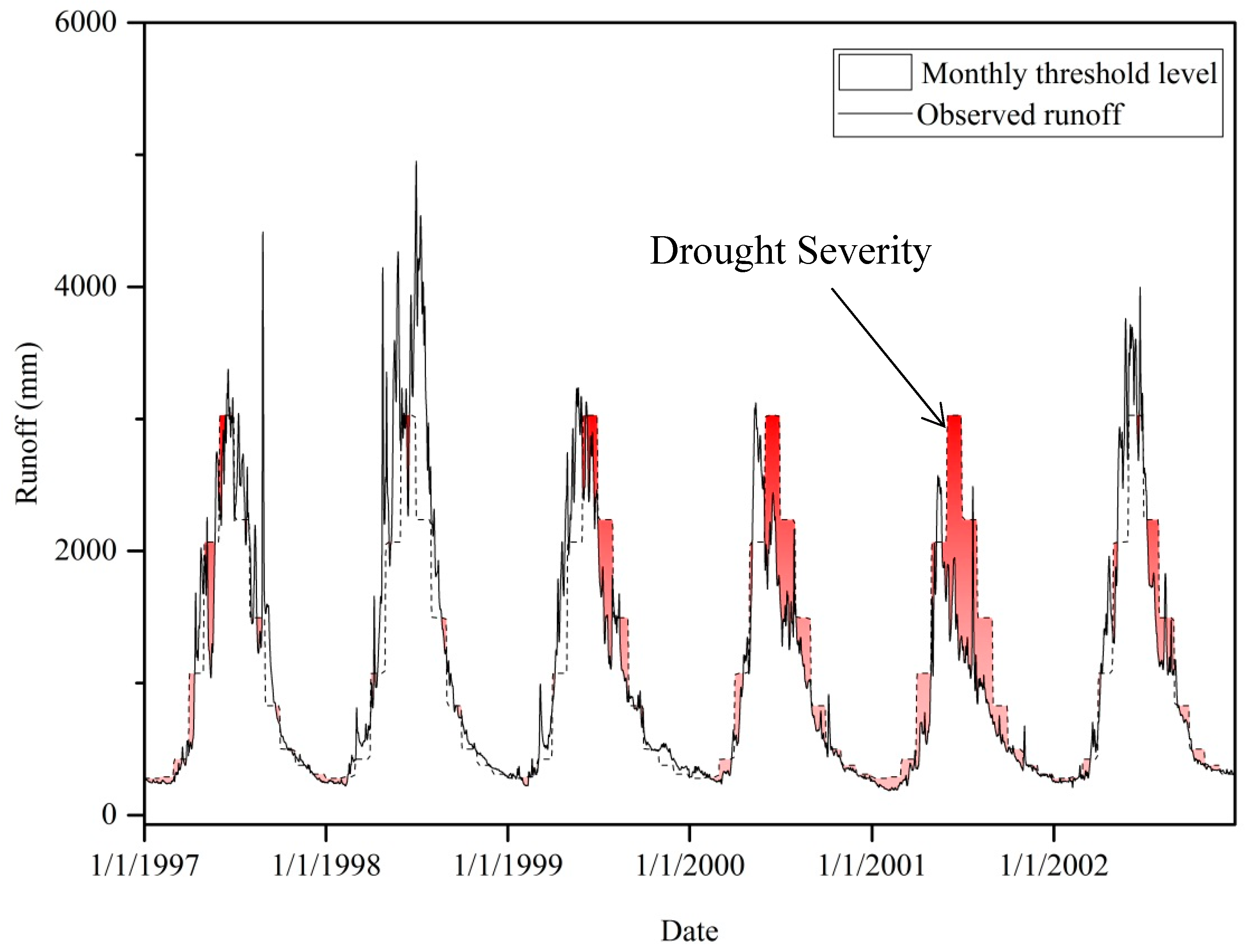
3.5. Hydrological Drought Analysis: 1961/1962–2009/2010

The duration and severity of hydrological drought events in the Kunhar River basin from 1961–2010 are shown in Figure 21, Figure 22, Figure 23 and Figure 24. More drought events occurred in Zone II than in Zone I, as shown in Figure 21 and Figure 22. Zone II had fixed and transient variable thresholds ranging between 87 and 151 days. The results obtained using the fixed and transient variable threshold approach clearly indicated that drought severity was greater in the lower region of the Kunhar River. There was a clear relationship between the number of drought events and their mean duration. Extreme and severe events were observed in Zone I in 1988, 1998, 2004–2006, and 2009–2010, with durations ranging between 106 and 131 days. Based on the transient variable threshold level, the duration of extreme events in Zone I was 221 and 206 days in 1998 and 1988, respectively. Based on the fixed threshold, the extreme and severe events had a severity of 204.58 mm in 1998 but, based on the monthly threshold level, the severity was 885.43 mm.
The fixed and transient variable threshold levels also indicate that frequent events had shorter durations in Zone I. Similar studies have reported the frequent occurrence of drought events with shorter durations. Drought events were found to be more severe than frequent events with shorter durations. The runoff amounts of 1969–1970, 1973, and 2001 were higher than the fixed threshold levels, while in Zone I in 1969 the transient variable threshold level was lower than the runoff amount. This pattern of drought events with longer durations can be attributed to both geographical morphology and atmospheric processes in these regions. It seems that, once a drought event has been established in this region, they have durations of between 11–117 days for the fixed Q80 threshold and 10–69 days for the transient variable threshold level. The severity of one-off drought events was in the range 9.01–204.58 mm for the fixed Q80 threshold and 73.93–709.20 mm for the transient variable threshold. The maximum severity of a single drought event was 247.82 mm in 1998 for the fixed Q80 threshold and 1705.36 mm in 2003 for the transient variable threshold. The duration and severity of all of the drought events were determined based on the fixed Q80 and transient variable thresholds.
The annual maxima of drought severity and the average drought duration are shown in Figure 23 and Figure 24, respectively. In the case of Zone II, the maximum duration occurred in 1985 (142 days) for the fixed Q80 threshold, and was 292 days in 2001 for the transient variable threshold. The average severity in this zone was 108.27 mm in 1993 for the fixed Q80 threshold and 447.67 mm in 2001 for the transient variable threshold. The maximum severity was 1882.54 mm in 2001 according to the transient threshold variable approach, while according to the fixed threshold level the maximum severity (260.66 mm) occurred in 1967 (Table 5). Frequent drought events had longer durations than single events in Zone II for the fixed Q80 threshold and were also more severe (49%) than single events. There was little difference (14%) between the maximum severity of single and multiple drought events at the fixed Q80 threshold. Frequent events had higher (50%) maximum severity than single events in the case of the transient variable threshold as shown in Figure 25 and Figure 26. Frequent and single events also had approximately the same average severity, of 203 and 201 mm, respectively, and average duration (88 and 32 days, respectively) at the transient variable threshold level. We also identified pooling due to the increased duration of drought events [15]. The correlation between the fixed-duration and transient variable thresholds was 0.5 and 0.8 for Zone I and Zone II, respectively, while the respective correlation of maximum severity was 0.78 and 0.28 for Zone I and II. The correlation of severity between the two zones was lower than that for duration. Small variations in the findings obtained using these two threshold levels have also been reported by other researchers [14,17,21,24,61].

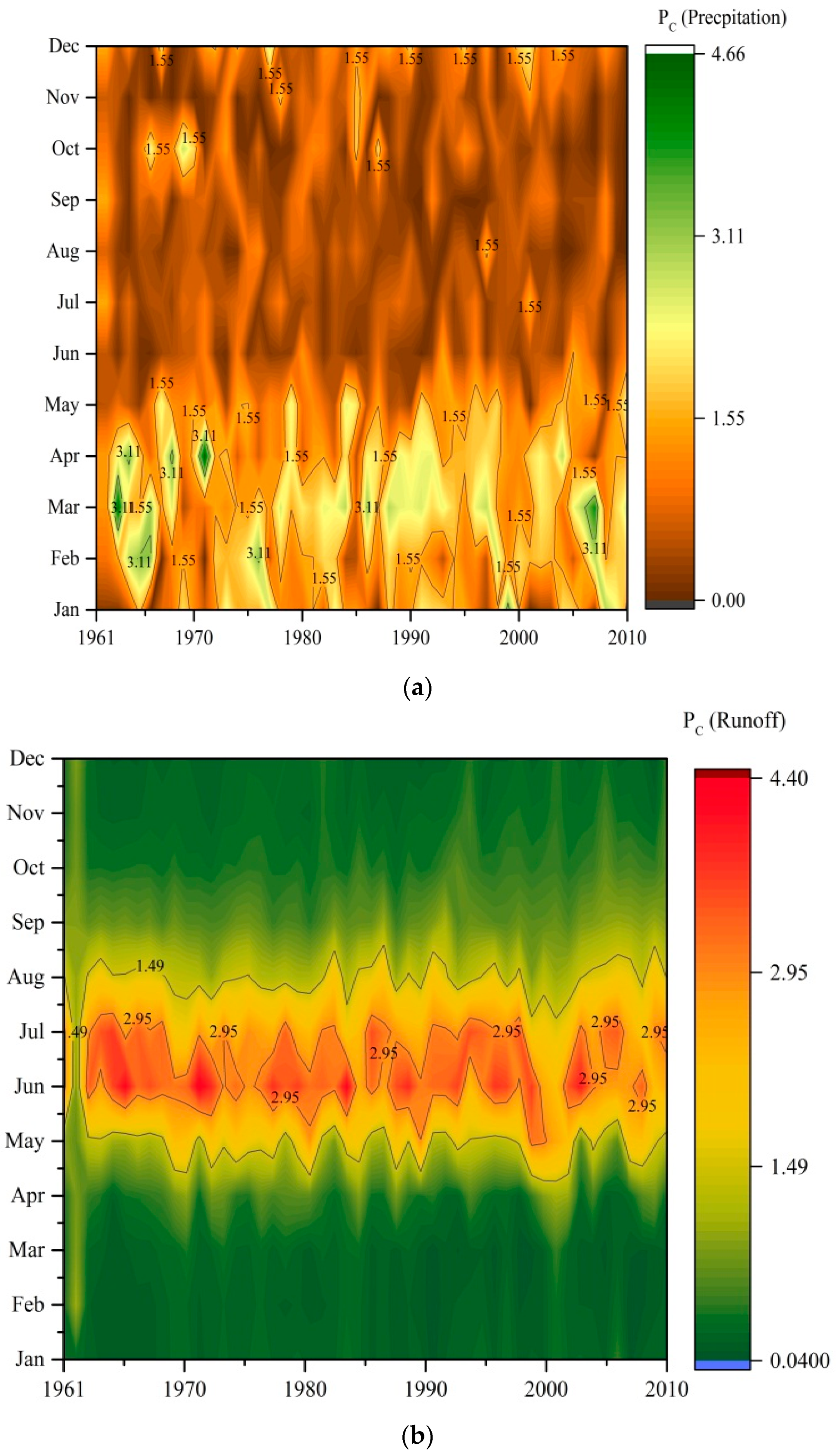
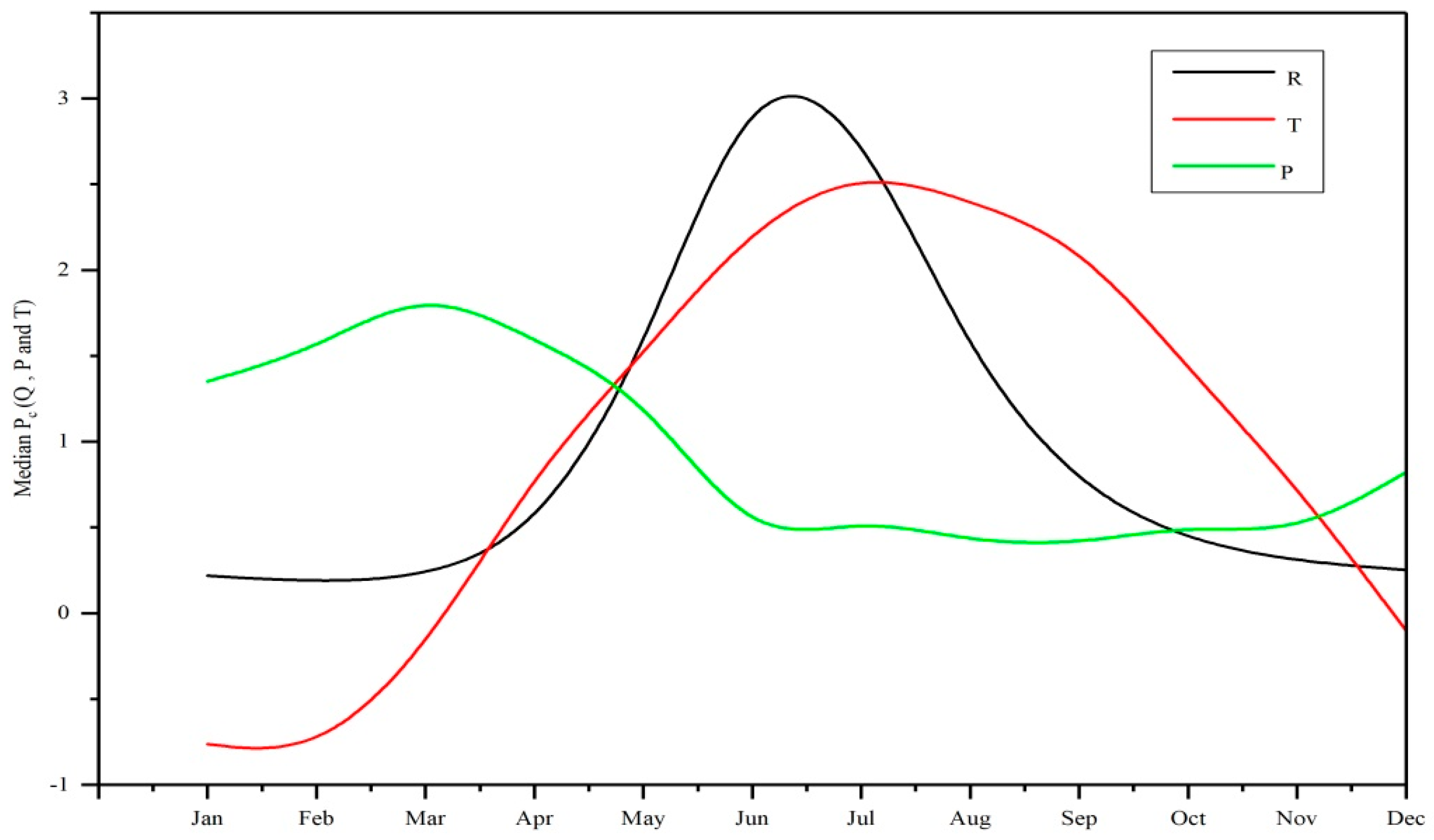
3.6. Sensitivity of Hydrological Regime to Climate

The runoff regime has been observed to be more consistent than the temperature regime, and there was a strong relationship between temperature and runoff in Zone I. This provides strong evidence that runoff varied in response to variations in temperature rather than precipitation. The hydrograph of Zone I also indicates the strength of the relationship between runoff and temperature, as shown in Figure 27 and Figure 28. The snow began to melt earlier in this zone. The inter-annual variability in the sensitivity of precipitation and temperature implies that runoff depended more on temperature than on precipitation. The temperature sensitivity value reached 0.62 in May, which implies that the snow melted earlier in Zone I. We evaluated the sensitivity of the runoff according to the temperature and precipitation and found that the increase in runoff in Zone I was primarily due to temperature. At the annual scale, positive precipitation elasticity and negative temperature elasticity indicated the dependency of the runoff on climatic factors.
Based on the results obtained from our models of the two zones, runoff was more sensitive to precipitation in Zone I than in Zone II. In Zone II, runoff depended on both precipitation and temperature. The overall runoff of the basin was also influenced by both precipitation and temperature.
We developed a two-parameter climate elasticity model of the two zones based on a new non-parametric method rather than a parametric method. The modified parametric model clearly shows the relationship between climatic factors and runoff, as indicated by the correlation coefficients, ratios, and standard deviations of the meteorology and hydrology factors. Most of the runoff was caused by melting of the snow pack, which plays a vital role in the hydrological process.
The precipitation and temperature values derived from models of Zone I and Zone II impacted the runoff characteristics of the Kunhar River basin. Climatic factors had the same effects in the two zones. We assessed the sensitivity of our non-parametric models to precipitation and temperature and found our non-parametric method to have several advantages over other non-parametric methods.
The sensitivity values of our models to precipitation and temperature in the two zones were 0.11, 0.23 and −0.04, −2.97, respectively. These results are similar to those reported for other regions [54]. The results obtained from the modified model were similar to previous results for other rivers i.e., Mary Darling basin (εp = 2.6, εET = −1.6) [58], Michigan basin (εp = 0.74–0.64, εET = −0.23–−0.31) [8], Miyun reservoir (εp = 2.27, εET = −0.79) [40] La source-de-chez-Pierre à Ceyssat River in France (εp = −0.31, εET = −3.04) [62] and different regions in the United States (εp = 0.79–1.82, εET = −0.15–0.26) [9]. The authors of reference [31] reported similar findings in a tributary of the Indus River (Soan River basin εp = 0.52, εET = −0.26). The authors of reference [37] stated that climate elasticity must be less than zero for precipitation and temperature to increase the stream flow of the Aksu River. The results of the modified climate elasticity model are consistent with those of other non-parametric methods, and with findings reported by other researchers [28,38,63].

4. Discussion

In this study, we developed a threshold-level-based approach for analyzing the hydrological regime of a high-altitude catchment in the western Himalayas using fixed and transient variable threshold levels. Fixed and transient variable thresholds were used to evaluate the characteristics of droughts in the study area. The standardized runoff index was not applied because it cannot determine the severity of runoff in a basin [17,24]. The deviation of the runoff from the threshold was assessed based on hydrological drought characteristics. We used this approach because the high-flow season is important for hydropower generation, where high-altitude catchments such as the one investigated in this study have strong hydropower generation potential [64,65]. The deviation from the threshold is governed by climate and weather patterns, which influence a range of hydrological events. We used 2D iso-plots of the hydrological regime to identify drought events in the study area. Similarly, trends in the hydrological regime also determine whether certain types of events occur in a catchment. Modified ITA statistics, Sen’s slopes (%) and iso-plots have never been plotted for this region in the context of practical significance levels.
We applied these statistical methods to identify certain types of events in this catchment. The key variables affecting the hydrological regime are precipitation and temperature, or their combination in high-altitude catchments [66], which is principle elements of climate change. Therefore, climate change is affecting the hydrological regime of this catchment [15,18]. The influence of precipitation and temperature varied within the study area, due to variation in altitude within the basin, and the accumulation of snow in Zone I of the western Himalayas. The authors of reference [44] investigated snow-cover dynamics at high altitudes in the western Himalayas. Snow cover and temperature were found to be negatively correlated at high altitudes, whereas precipitation was positively correlated with snow cover. The snow-cover area of this region decreased between 2000 and 2009 and was negatively correlated with stream flow. The high-altitude snow cover affects the hydrological regime of the western Himalayas. Winter precipitation expands the snow-cover area, which is then reduced by increases in summer temperatures (Figure 29). The authors of reference [67] investigated snow water equivalent in different villages of the high-altitude basin and found that it was highly correlated with stream flow at Narran and Garhi Habibullah. They also observed that the snow water equivalent varied with altitude, and its relationship with stream flow strengthened with increasing elevation. The elevation of the catchment affected the temperature, with lower temperatures observed in more elevated areas, which were covered with glaciers and snow. Snow and glaciers increase the severity of droughts. The effect of altitude becomes negligible without snow and glacier cover [2]. The authors of reference [43] also investigated the impact of climate on the hydrological regime of the western Himalayas and reported that temperature and precipitation play major roles in the hydrological regime. Snow-melting processes in the high-altitude catchment are governed by temperature and precipitation.
Analyzing sensitivity to precipitation and temperature can help researchers to understand extreme events in river basins. Therefore, many researchers have investigated the climate sensitivity of hydrological regimes [19,54,57,68], but some important variables have never have been taken into account when estimating the sensitivity of runoff to precipitation and temperature. Weather circulation patterns also play a key role and have a large impact on snow in the catchment. Temperature and precipitation contribute to both normal hydrological conditions and specific events. The large elevation range of the catchment also causes the hydrological regime variables to be below threshold levels in certain areas, because the temperature and precipitation gradients produce uncertainty. Precipitation and temperature sensitivity affect the hydrological regime. This sensitivity can also lead to variations in threshold levels over the entire basin and increases the altitude at which snow melts, which in turn leads to shifts in the hydrological regime. Events that previously ended at the end of the snow-melt season can now continue into summer. This has strong implications for water-resource management in high-altitude catchments.

5. Conclusions

In this study, we used historical meteorological and hydrological data to evaluate the threshold levels and sensitivity of the hydrological regime of the western Himalayas to temperature and precipitation, at high altitudes. This area is a major tributary of the Mangla reservoir. We carried out several hydrological regime analyses, based on which we drew the following conclusions:
1. The annual runoff in the two zones is decreasing, in contrast to the precipitation and temperature. Precipitation increased in Zone I at the 10% practical significance level, while the temperature increased in both zones.
2. We plotted our data and found that the hydrological regime was more sensitive to temperature than to precipitation during the high-runoff months of the study period (1961–2010). This was the case in both zones in the high-altitude region of the western Himalayas. The iso-plots of the Pardé coefficients of the runoff enabled us to identify extreme events in the basin. Hence, this method is more informative than traditional methods.
3. We identified drought events in the hydrological regime at high altitudes in the western Himalayas. We defined fixed and monthly threshold levels so that we could calculate the severity and duration of droughts in the two zones. Based on the fixed and transient threshold levels developed for the entire basin, we found that drought severity was higher in Zone I than in Zone II.
4. Runoff was more sensitive to temperature in Zone I, while precipitation and temperature played a combined role in Zone II. During June, July, and August, the temperature in Zone I caused the runoff to the entire basin to increase. In the case of Zone II, precipitation caused increased runoff and the temperature of the zone decreased.
The results of the above analyses indicate that, should such hydrological conditions persist, water-shortage problems in Pakistan will become more severe, especially in high-altitude areas, where the temperature is increasing. Snow and glaciers are melting due to increasing temperatures. More observations from higher elevations of the western Himalayas are needed for comparison with records held by the valley base stations. This will provide researchers with a more accurate climate record for this area.

Author Contributions

S.L. supervised and designed this study. M.S. processed the data and wrote the manuscript. A.A.T., M.A. (Muhammad Ashraf) and S.A. helped to draft the manuscript. A.M. and M.Z. helped to solve the issue of statistics and trend analysis. M.A. (Muhammad Adnan) and D.C. helped to solve the problems of climate sensitivity model and drought analysis.

Funding

This research was funded by joint Research project of National Natural Science Foundation of China and International Center for Integrated Mountain Development NSFC-ICIMOD (Grant No. 41761144075), Higher Education Commission (HEC) of Pakistan (HEC/STR/279), China Postdoctoral Science Foundation (Grant No. 209071) and Yunnan University (YJRC3201702).

Acknowledgments

We are thankful to PMD and WAPDA providing the observed metrological and hydrological data. We are thankful to editor and associate editor, as well as reviewers for their valuable comments and suggestions to improve this manuscript.

Conflicts of Interest

The authors declare no conflict of interests.

Appendix A

Mann–Kendall test
The MK test static (S) of variables is calculated in the following Equations:
S = i = 1 n 1 j = i + 1 n sgn ( x j x i )
where
sgn ( x j x i ) = { + 1 ,     x j > x i     0 ,     x j = x i 1 ,     x j < x i
where xi and xj are time series at times i and j, n represent the length of the time series.
The following expression is used for the given time series:
V ( S ) = n ( n 1 ) ( 2 n + 5 ) i = 1 n t i i ( i 1 ) ( 2 i + 5 ) 18
where ti is the number of data values. The standard z value is calculated according to the following:
z = { S 1 var ( S )       S > 0 0                           S = 0 S 1 var ( S )       S < 0
The standard z value is compared with standard normal distribution table with a two tailed test at significance level (α = 10%, α = 5%, α = 1%).
Sen.’s slope estimator
The slope of n pairs is estimated as:
β i = median [ X J X K J K ]
where Xj and Xk represent the value at time j and k respectively.
For odd number, sen slope can be computed as:
β med = β ( n + 1 ) / 2
For even n number, slope can be estimated as:
β med = 1 2 ( β ( n ) / 2 + β ( n + 2 ) / 2 )

References

  1. Mahmood, R.; Jia, S.; Babel, M. Potential Impacts of Climate Change on Water Resources in the Kunhar River Basin, Pakistan. Water 2016, 8, 23. [Google Scholar] [CrossRef]
  2. Tahir, A.A.; Chevallier, P.; Arnaud, Y.; Ashraf, M.; Bhatti, M.T. Snow cover trend and hydrological characteristics of the Astore River basin (Western Himalayas) and its comparison to the Hunza basin (Karakoram region). Sci. Total Environ. 2015, 505, 748–761. [Google Scholar] [CrossRef] [PubMed]
  3. Shrestha, M.; Koike, T.; Hirabayashi, Y.; Xue, Y.; Wang, L.; Rasul, G.; Ahmad, B. Integrated simulation of snow and glacier melt in water and energy balance-based, distributed hydrological modeling framework at Hunza River Basin of Pakistan Karakoram region. J. Geophys. Res. Atmos. 2015, 4889–4919. [Google Scholar] [CrossRef]
  4. Farhan, S.B.; Zhang, Y.; Aziz, A.; Gao, H.; Ma, Y.; Kazmi, J.; Nasir, J.; Shahzad, A.; Hussain, L.; Mansha, M.; et al. Assessing the impacts of climate change on the high altitude snow- and glacier-fed hydrological regimes of Astore and Hunza, the sub-catchments of Upper Indus Basin. J. Water Clim. Chang. 2018. [Google Scholar] [CrossRef]
  5. Zheng, H.; Zhang, L.; Zhu, R.; Liu, C.; Sato, Y.; Fukushima, Y. Responses of streamflow to climate and land surface change in the headwaters of the Yellow River Basin. Water Resour. Res. 2009, 45. [Google Scholar] [CrossRef]
  6. Merz, R.; Blöschl, G. A regional analysis of event runoff coefficients with respect to climate and catchment characteristics in Austria. Water Resour. Res. 2009, 45. [Google Scholar] [CrossRef] [Green Version]
  7. Zou, L.; Xia, J.; She, D. Analysis of Impacts of Climate Change and Human Activities on Hydrological Drought: A Case Study in the Wei River Basin, China. Water Resour. Manag. 2017, 32, 1421–1438. [Google Scholar] [CrossRef]
  8. Zhang, Y.; Engel, B.; Ahiablame, L.; Liu, J. Impacts of Climate Change on Mean Annual Water Balance for Watersheds in Michigan, USA. Water 2015, 7, 3565–3578. [Google Scholar] [CrossRef]
  9. Tsai, Y. The multivariate climatic and anthropogenic elasticity of streamflow in the Eastern United States. J. Hydrol. Reg. Stud. 2017, 9, 199–215. [Google Scholar] [CrossRef]
  10. Milano, M.; Reynard, E.; Bosshard, N.; Weingartner, R. Simulating future trends in hydrological regimes in Western Switzerland. J. Hydrol. Reg. Stud. 2015, 4, 748–761. [Google Scholar] [CrossRef] [Green Version]
  11. Zelenhasić, E.; Salvai, A. A Method of Streamflow Drought Analysis. Water Resour. Res. 1987, 23, 156–168. [Google Scholar] [CrossRef]
  12. Carroll, N.; Frijters, P.; Shields, M.A. Quantifying the costs of drought: New evidence from life satisfaction data. J. Popul. Econ. 2009, 22, 445–461. [Google Scholar] [CrossRef]
  13. Wanders, N.; Wada, Y. Human and climate impacts on the 21st century hydrological drought. J. Hydrol. 2015, 526, 208–220. [Google Scholar] [CrossRef]
  14. Rivera, J.A.; Araneo, D.C.; Penalba, O.C. Threshold level approach for streamflow drought analysis in the Central Andes of Argentina: A climatological assessment. Hydrol. Sci. J. 2017, 62, 1949–1964. [Google Scholar] [CrossRef]
  15. Van Loon, A.F.; Laaha, G. Hydrological drought severity explained by climate and catchment characteristics. J. Hydrol. 2015, 526, 3–14. [Google Scholar] [CrossRef] [Green Version]
  16. Saifullah, M.; Li, Z.; Li, Q.; Zaman, M.; Hashim, S. Quantitative Estimation of the Impact of Precipitation and Land Surface Change on Hydrological Processes through Statistical Modeling. Adv. Meteorol. 2016, 2016, 1–15. [Google Scholar] [CrossRef] [Green Version]
  17. Sung, J.H.; Chung, E.S. Development of streamflow drought severity–duration–frequency curves using the threshold level method. Hydrol. Earth Syst. Sci. 2014, 18, 3341–3351. [Google Scholar] [CrossRef]
  18. Liu, Y.; Ren, L.; Zhu, Y.; Yang, X.; Yuan, F.; Jiang, S.; Ma, M. Evolution of Hydrological Drought in Human Disturbed Areas: A Case Study in the Laohahe Catchment, Northern China. Adv. Meteorol. 2016, 2016, 1–12. [Google Scholar] [CrossRef]
  19. Jiang, S.; Ren, L.; Yong, B.; Singh, V.P.; Yang, X.; Yuan, F. Quantifying the effects of climate variability and human activities on runoff from the Laohahe basin in northern China using three different methods. Hydrol. Process. 2011, 25, 2492–2505. [Google Scholar] [CrossRef]
  20. Tsakiris, I.N.G. Assessment of Hydrological Drought Revisited. Water Resour. Manag. 2009, 881–897. [Google Scholar] [CrossRef]
  21. Van Loon, A.F.; Van Lanen, H.A.J. A process-based typology of hydrological drought. Hydrol. Earth Syst. Sci. 2012, 16, 1915–1946. [Google Scholar] [CrossRef] [Green Version]
  22. Razmkhah, H. Comparing Threshold Level Methods in Development of Stream Flow Drought Severity-Duration-Frequency Curves. Water Resour. Manag. 2017, 31, 4045–4061. [Google Scholar] [CrossRef]
  23. Tallaksen, L.M.; Madsen, H.; Clausen, B. On the definition and modelling of streamflow drought duration and deficit volume. Hydrol. Sci. J. 1997, 42, 15–33. [Google Scholar] [CrossRef]
  24. Khan, M.I.; Liu, D.; Fu, Q.; Faiz, M.A. Detecting the persistence of drying trends under changing climate conditions using four meteorological drought indices. Meteorol. Appl. 2018, 25, 184–194. [Google Scholar] [CrossRef]
  25. Kjeldsen, T.R.; Lundorf, A.; Rosbjerg, D. Use of a two-component exponential distribution in partial duration modelling of hydrological droughts in Zimbabwean rivers. Hydrol. Sci. J. 2000, 45, 285–298. [Google Scholar] [CrossRef]
  26. Sankarasubramanian, A.; Vogel, R.M. Annual hydro climatology of the United States. Water Resour. Res. 2002, 38, 19-1–19-12. [Google Scholar] [CrossRef]
  27. Bormann, H. Runoff regime changes in German rivers due to climate change. Erdkunde 2010, 64, 257–279. [Google Scholar] [CrossRef]
  28. Wang, S.; Yan, Y.; Yan, M.; Zhao, X. Quantitative estimation of the impact of precipitation and human activities on runoff change of the Huangfuchuan River Basin. J. Geogr. Sci. 2012, 22, 906–918. [Google Scholar] [CrossRef]
  29. Sankarasubramanian, A.; Vogel, R.M.; Limbrunner, J.F. Climate elasticity of streamflow in the United States. Water Resour. Res. 2001, 37, 1771–1781. [Google Scholar] [CrossRef]
  30. Saifullah, M.; Li, Z.; Li, Q.; Hashim, S.; Zaman, M. Quantifying the Hydrological Response to Water Conservation Measures and Climatic Variability in the Yihe River Basin, China. Outlook Agric. 2015, 44, 273–282. [Google Scholar] [CrossRef]
  31. Shahid, M.; Cong, Z.; Zhang, D. Understanding the impacts of climate change and human activities on streamflow: A case study of the Soan River basin, Pakistan. Theor. Appl. Climatol. 2017, 134, 205–219. [Google Scholar] [CrossRef]
  32. Zhai, R.; Tao, F. Contributions of climate change and human activities to runoff change in seven typical catchments across China. Sci. Total Environ. 2017, 605–606, 219–229. [Google Scholar] [CrossRef]
  33. Xu, Y.; Wang, S.; Bai, X.; Shu, D.; Tian, Y. Runoff response to climate change and human activities in a typical karst watershed, SW China. PLoS ONE 2018, 13, e0193073. [Google Scholar] [CrossRef]
  34. Saifulllah, M.; Li, Z.J.; Li, Q.L.; Hashim, S.; Zaman, M.; Liu, K.L. Assessment the impacts of land surface change on the hydrological process based on similar hydro-meteorological conditions with SWAT. Fresenius Environ. Bull. 2016, 25, 3071–3082. [Google Scholar]
  35. Li, B.; Su, H.; Chen, F.; Li, H.; Zhang, R.; Tian, J.; Chen, S.; Yang, Y.; Rong, Y. Separation of the impact of climate change and human activity on streamflow in the upper and middle reaches of the Taoer River, northeastern China. Theor. Appl. Climatol. 2013, 118, 271–283. [Google Scholar] [CrossRef]
  36. Li, B.; Chen, F. Using the aridity index to assess recent climate change: A case study of the Lancang River Basin, China. Stoch. Environ. Res. Risk Assess. 2014, 29, 1071–1083. [Google Scholar] [CrossRef]
  37. Kundzewicz, Z.W.; Merz, B.; Vorogushyn, S.; Hartmann, H.; Duethmann, D.; Wortmann, M.; Huang, S.; Su, B.; Jiang, T.; Krysanova, V. Analysis of changes in climate and river discharge with focus on seasonal runoff predictability in the Aksu River Basin. Environ. Earth Sci. 2014, 73, 501–516. [Google Scholar] [CrossRef] [Green Version]
  38. Wang, W.; Zhang, Z.; Duan, L.; Wang, Z.; Zhao, Y.; Zhang, Q.; Dai, M.; Liu, H.; Zheng, X.; Sun, Y. Response of the groundwater system in the Guanzhong Basin (central China) to climate change and human activities. Hydrogeol. J. 2018, 26, 1429–1441. [Google Scholar] [CrossRef]
  39. Chiew, F.H.; Peel, M.C.; McMahon, T.A.; Siriwardena, L.W. Precipitation elasticity of streamflow in catchments across the world. Climate Variability and Change—Hydrological Impacts. In Proceedings of the Fifth Friend World Conference, Havana, Cuba, 27 November–1 December 2006. [Google Scholar]
  40. Ma, H.; Yang, D.; Tan, S.K.; Gao, B.; Hu, Q. Impact of climate variability and human activity on streamflow decrease in the Miyun Reservoir catchment. J. Hydrol. 2010, 389, 317–324. [Google Scholar] [CrossRef]
  41. Forsythe, N.; Fowler, H.J.; Blenkinsop, S.; Burton, A.; Kilsby, C.G.; Archer, D.R.; Harphamc, C.; Hashmi, M.Z. Application of a stochastic weather generator to assess climate change impacts in a semi-arid climate: The Upper Indus Basin. J. Hydrol. 2014, 517, 1019–1034. [Google Scholar] [CrossRef] [Green Version]
  42. Mahmood, R.; Babel, M.S. Evaluation of SDSM developed by annual and monthly sub-models for downscaling temperature and precipitation in the Jhelum basin, Pakistan and India. Theor. Appl. Climatol. 2013, 113, 27–44. [Google Scholar] [CrossRef]
  43. Babur, M.; Babel, M.; Shrestha, S.; Kawasaki, A.; Tripathi, N. Assessment of Climate Change Impact on Reservoir Inflows Using Multi Climate-Models under RCPs—The Case of Mangla Dam in Pakistan. Water 2016, 8, 389. [Google Scholar] [CrossRef]
  44. Azmat, M.; Liaqat, U.W.; Qamar, M.U.; Awan, U.K. Impacts of changing climate and snow cover on the flow regime of Jhelum River, Western Himalayas. Reg. Environ. Chang. 2017, 17, 813–825. [Google Scholar] [CrossRef]
  45. Şen, Z. Innovative Trend Analysis Methodology. J. Hydrol. Eng. 2012, 17, 1042–1046. [Google Scholar] [CrossRef]
  46. Şen, Z. Trend Identification Simulation and Application. J. Hydrol. Eng. 2014, 19, 635–642. [Google Scholar] [CrossRef]
  47. Saplıoğlu, K.; Kilit, M.; Yavuz, B.K. Trend analysis of streams in the western Mediterranean basin of Turkey. Fresenius Environ. Bull. 2014, 23, 1–12. [Google Scholar]
  48. Yue, S.; Hashino, M. Long term trends of annual and monthly precipitation in Japan. Am. Water Resour. Assoc. 2003, 39, 587–596. [Google Scholar] [CrossRef]
  49. Mann, H. Nonparametric Tests against Trend. Econometrica 1945, 13, 245–259. [Google Scholar] [CrossRef]
  50. Sen, P.K. Estimates of the Regression Coefficient Based on Kendall’s Tau. J. Am. Stat. Assoc. 1968, 63, 1379–1389. [Google Scholar] [CrossRef]
  51. Theil, H. A rank-invariant method of linear and polynomial regression analysis. Mathematics 1992, 23, 345–381. [Google Scholar]
  52. Pardé, M. Quelques notes sur l’hydrologie du Brahmapoutre, du Gange et de l’Indus. Revue de. Géographie Alpine 1940, 28, 157–198. [Google Scholar] [CrossRef]
  53. Parde, M. Fleuves et Rivières. Rev. Géogr. Alp. 1933, 214, 851–854. [Google Scholar]
  54. Amo-Boateng, M.; Li, Z.; Guan, Y. Inter-annual variation of streamflow, precipitation and evaporation in a small humid watershed (Chengcun Basin, China). Chin. J. Oceanol. Limnol. 2013, 32, 455–468. [Google Scholar] [CrossRef]
  55. Hao, X.; Chen, Y.; Xu, C.; Li, W. Impacts of Climate Change and Human Activities on the Surface Runoff in the Tarim River Basin over the Last Fifty Years. Water Resour. Manag. 2007, 22, 1159–1171. [Google Scholar] [CrossRef]
  56. Yao, J.Q.; Zhao, Q.D.; Liu, Z.H. Effect of climate variability and human activities on runoff in the Jinghe River Basin, Northwest China. J. Mt. Sci. 2015, 12, 358–367. [Google Scholar] [CrossRef]
  57. Fu, G.; Charles, S.P.; Chiew, F.H. A two-parameter climate elasticity of streamflow index to assess climate change effects on annual streamflow. Water Resour. Res. 2007, 43. [Google Scholar] [CrossRef]
  58. Roderick, M.L.; Farquhar, G.D. A simple framework for relating variations in runoff to variations in climatic conditions and catchment properties. Water Resour. Res. 2011, 47. [Google Scholar] [CrossRef]
  59. Mátyás, K.; Bene, K. Comparison of Annual Prediction Methods for Spring Flow in the Aggtelek Region. Acta Tech. Jaurinensis 2017, 10, 70–73. [Google Scholar] [CrossRef]
  60. Olsson, O.; Gassmann, M.; Wegerich, K.; Bauer, M. Identification of the effective water availability from streamflows in the Zerafshan river basin, Central Asia. J. Hydrol. 2010, 390, 190–197. [Google Scholar] [CrossRef]
  61. Rasul, G. Climate Data Modelling and Analysis of the Indus Ecoregion; World Wide Fund Nature Pak: Lahore, Pakistan, 2012; pp. 26–27. [Google Scholar]
  62. Andréassian, V.; Coron, L.; Lerat, J.; Le Moine, N. Climate elasticity of streamflow revisited—An elasticity index based on long-term hydrometeorological records. Hydrol. Earth Syst. Sci. 2016, 20, 4503–4524. [Google Scholar] [CrossRef]
  63. Wang, D.; Alimohammadi, N. Responses of annual runoff, evaporation, and storage change to climate variability at the watershed scale. Water Resour. Res. 2012, 48. [Google Scholar] [CrossRef] [Green Version]
  64. Khan, M.; Zaidi, A.Z. Run-of-River Hydropower Potential of Kunhar River, Pakistan. Pakistan J. Meteorol. 2015, 12, 25–32. [Google Scholar]
  65. Ali, A.F.; Zhang, X.P.; Adnan, M.; Iqbal, M.; Khan, G. Projection of future streamflow of the Hunza River Basin, Karakoram Range (Pakistan) using HBV hydrological model. J. Mt. Sci. 2018, 15, 2218–2235. [Google Scholar] [CrossRef]
  66. Saifullah, M.; Zaman, M.; Li, Z.; Nasir, A. Impacts of hydro climatic variables trends on water resources of Yihe River Basin during the past 50 years. In Proceeding of the International Conference on Hydropower—A Vital Source of Sustainable Energy for Pakistan 2017, Washington, DC, USA, 19–20 December 2017; pp. 42–46. [Google Scholar]
  67. De Scally, F.A. Relative importance of snow accumulation and monsoon rainfall data for estimating annual runoff, Jhelum basin, Pakistan. Hydrol. Sci. 1994, 39, 199–216. [Google Scholar] [CrossRef]
  68. Chen, X.; Alimohammadi, N.; Wang, D. Modeling inter-annual variability of seasonal evaporation and storage change based on the extended Budyko framework. Water Resour. Res. 2013, 49, 6067–6078. [Google Scholar] [CrossRef]
Figure 1. High altitude catchment of western Himalaya, Pakistan.
Water 11 01454 g001
Figure 2. Box plot and distribution of precipitation, runoff and temperature Zone I. (a) monthly precipitation, (b) monthly runoff, (c) monthly temperature, (d) annual runoff, precipitation and temperature.
Water 11 01454 g002aWater 11 01454 g002b
Figure 3. Box plot and distribution of precipitation, runoff and temperature of Zone II (a) monthly precipitation, (b) monthly runoff, (c) monthly temperature, (d) annual runoff, precipitation and temperature.
Water 11 01454 g003aWater 11 01454 g003b
Figure 4. Illustration of decreasing, increasing and trendless region in the hydrological time series.
Water 11 01454 g004
Figure 5. Sketch of methodology for threshold levels for hydrological regime.
Water 11 01454 g005
Figure 6. Transient threshold variable method for analyzing pooled events for the daily hydrological data.
Water 11 01454 g006
Figure 7. Comparison of Mann–Kendall (MK) trends of (a) precipitation, (b) runoff and (c) temperature of Zones I and II.
Water 11 01454 g007aWater 11 01454 g007b
Figure 8. Annual innovative trend analysis (ITA) statistics for precipitation, runoff and temperature for Zone II. (a) precipitation, (b) runoff, (c). temperature.
Water 11 01454 g008
Figure 9. Annual ITA of Precipitation, runoff and temperature Zone I. (a) Precipitation (b) runoff (c). temperature.
Water 11 01454 g009aWater 11 01454 g009b
Figure 10. Iso-plot of precipitation, runoff and temperature of Zone I. (a) precipitation (b) runoff (c) temperature.
Water 11 01454 g010
Figure 11. Inter-annual variability of temperature, precipitation and runoff for Zone I.
Water 11 01454 g011
Figure 12. Contour plot of the precipitation, runoff and temperature for Zone II. (a) precipitation (b) runoff (c) temperature.
Water 11 01454 g012
Figure 13. Inter-annual variability of the temperature, precipitation and runoff for Zone II.
Water 11 01454 g013
Figure 14. Contours of Parde co-efficient precipitation, runoff and temperature of zone I. (a) precipitation (b) runoff (c) temperature.
Water 11 01454 g014aWater 11 01454 g014b
Figure 15. Contours of Parde co-efficient of precipitation, runoff and temperature of Zone II. (a) precipitation (b) runoff (c) temperature.
Water 11 01454 g015aWater 11 01454 g015b
Figure 16. Comparison of different parameters of zone I.
Water 11 01454 g016
Figure 17. Comparison of different parameters of Zone II.
Water 11 01454 g017
Figure 18. Accumulative deviation curve for runoff, precipitation and temperature for Zone I.
Water 11 01454 g018
Figure 19. Accumulative deviation curve for runoff, precipitation and temperature for Zone II.
Water 11 01454 g019
Figure 20. Fixed and monthly threshold levels for both zones. (a) Fixed (b) monthly threshold levels
Water 11 01454 g020
Figure 21. Annual number of drought events in Zone I.
Water 11 01454 g021
Figure 22. Annual number of drought events in Zone II.
Water 11 01454 g022
Figure 23. Annual duration and average severities of Zone I. (a) Drought duration (b) Drought Severities.
Water 11 01454 g023
Figure 24. Annual duration and average severities of Zone II. (a) Drought duration (b) Drought Severities.
Water 11 01454 g024
Figure 25. Example of drought analysis based on transient threshold levels for the Zone I.
Water 11 01454 g025
Figure 26. Example of drought analysis based on transient threshold levels for the Zone II.
Water 11 01454 g026
Figure 27. Precipitation and temperature sensitivity of both zones. (a) Precipitation sensitivity (b) temperature sensitivity.
Water 11 01454 g027
Figure 28. Precipitation and temperature sensitivity in the two zones based on a modified climate-elasticity model. (a) Precipitation sensitivity (b) temperature sensitivity
Water 11 01454 g028
Figure 29. Snow characteristics of the western Himalayas.
Water 11 01454 g029
Table 1. Hydro-meteorological stations in the study area.
Sr. #StationLat (°N)Long (°E)Altitude (m ASL)Period (Years)
Meteorological station
1Naran34.973.6524211961–2010
2Balakot34.5573.35995Same period
3Muzzafarabad34.3773.48702Same period
Hydrological station
1Naran34.973.6523621961–2010
2Gari Habibullah34.4073.38810Same period
Table 2. Summary of the trend analysis for Zone I.
Monthβ (%)S (%)ITA
RPTRPTRPT
Jan−17.9242.8−1.06−2.0736.64−0.09
Feb−38.6562.5−2.19−4.1115.13−0.20
Mar−76.1857.3−2.45−6.3916.86−0.28
Apr−29.4050.8−0.63−1.1521.27−0.19
May6.1126.50.530.0829.820.02
Jun−31.7567.90.68−0.1215.130.14
Jul−29.8362.20.92−0.0438.480.12
Aug−17.3340.81.830.0338.420.19
Sep1.18−5.71.050.5918.630.12
Oct14.14−22.40.601.68−1.380.07
Nov17.7760.01.122.2850.460.11
Dec1.1150.20.64−0.2339.810.08
annual−16.1158.90.16−0.1230.280.01
Note: Runoff is denoted by R, Precipitation is denoted by, P Temperature is denoted by T. Bold letter represents practical significant level at 10%. Underline represents the significant trends of Modify innovative trend analysis (MITA), which cannot identify with others methods.
Table 3. Summary of the trend analysis of Zone II.
Monthβ (%)S (%)ITA
RPTRPTRPT
Jan−0.22−11.250.111.12−6.360.02
Feb8.67−14.130.161.58−2.180.02
Mar24.46−31.310.001.31−2.56−0.02
Apr16.60−60.920.210.25−11.000.00
May30.07−12.530.350.31−10.730.01
Jun−21.1737.84−0.50−0.11−3.28−0.03
Jul−17.79−4.390.12−0.03−0.290.08
Aug−17.55−14.500.020.01−2.370.00
Sep−13.07−1.200.240.665.160.02
Oct−8.38−16.980.251.93−11.360.01
Nov−4.690.000.361.5318.300.05
Dec−2.34−34.320.431.850.630.04
annual−2.56−15.040.170.14−3.160.01
Note: Runoff is denoted by R, P is denoted by Precipitation, T is denoted by Temperature. Bold letter represent practical significant level at 10%. Underline represent the significant trends of Modify innovative trend analysis (MITA), which cannot identify with others methods.
Table 4. Comparison of the amplitudes of various parameters in Zones I and II.
MonthRunoff Amplitude (RA)Precipitation Amplitude (PA)Temperature Amplitude (TA)
Zone IZone IIZone IZone IIZone IZone II
Jan0.410.203.391.903.260.23
Feb1.050.213.242.963.320.34
March0.860.444.042.423.040.37
April0.941.154.452.192.820.31
May2.491.532.491.172.480.40
June3.551.471.592.102.650.36
July2.671.571.565.312.250.24
August1.291.031.763.723.200.18
Sep0.701.621.552.542.720.23
Oct0.540.872.732.201.860.21
Nov0.580.321.811.241.710.35
Dec0.800.222.691.901.820.22
Table 5. Summary of the results based on fixed and transient variable thresholds.
ParametersFixed MethodVariable Method
Q80Monthly
IIIIII
Total drought events4687140151
No. of drought per year0.91.742.83.02
Mean duration (days)78.2863.6426.3978.98
Max duration (days)153142138292
Mean severity (mm)79.9555.61270.11207.64
Max severity (mm)285.16260.662539.021882.54

