Assessment of Field Water Uniformity Distribution in a Microirrigation System Using a SCADA System

Abstract

Microirrigation is an efficient irrigation technique, although when wastewater is used the probability of operation problems such as emitter clogging increases. In most of microirrigation systems, control of irrigation performance is manual and sporadic, therefore clogging problems may not be detected at the right time. As it is easier to prevent emitter clogging if it is detected earlier, close monitoring of pressure and flow rates in microirrigation systems is an important way to achieve microirrigation system requirements and accomplish higher irrigation efficiencies. A supervisory control and data acquisition (SCADA) system was used to monitor and control the performance of three microirrigation subunits; each one with four laterals, 90 m long with 226 emitters. The SCADA system monitored the pressure and flow across the irrigation laterals, and distribution uniformity coefficients were determined in real time, as they are indexes commonly used for evaluating drip irrigation systems. Results were compared with those experimentally obtained, showing a good correlation; although the emitter position had an important effect on the computed values. This work shows that a SCADA system can be easily used to continuously assess the pressure and water distribution uniformity without carrying out time-consuming manual field assessments.

1. Introduction

Microirrigation is the slow application of water on, above, or below the soil by surface drip, subsurface drip, bubbler, and microsprinkler systems [1]. Microirrigation has experienced an important growth over the past few decades, especially in developing countries [2] due to the need to save water since it is a technique that allows high irrigation efficiency, from 85 to 95% [1]. Moreover, microirrigation is the most appropriate technique for applying wastewater from both health and environmental points of view [3,4], in addition to being a viable alternative to deal with water scarcity [5], being especially important in areas with water scarcity.

One of the most commonly used parameters when designing and evaluating microirrigation systems is distribution uniformity (DU) [6]. DU expresses the variation of the emitter discharge of the irrigation system, which mainly depends on the hydraulic design, the coefficient of manufacturing variation, and emitter clogging [6,7]. Besides, DU allows detection and assessment of differences in water application and distribution in the crop and determining the causes, being able to reduce them and keep the irrigation system as close as possible to the uniformity system it was designed for [7]. For this reason, a regular evaluation of the irrigation system is also recommended.

Whenever the manufacturer’s coefficient of variation (CVm) and the evaluated system installation is adequate, the DU is a good indicator of emitter clogging, which is one of the most common problems in microrrigation systems. Emitter clogging can have physical, chemical, and biological causes, and can be especially important when low quality water such as wastewater is used [3,8].

One of the most frequent methods to determine the flow distribution uniformity coefficient (DU_lq) is that proposed by Merriam and Keller [9], which was also adopted by the Food and Agriculture Organization of the United Nations FAO [10]. The Merriam and Keller [9] method selects four locations of a secondary branch, one at the beginning, another at the end and the other two between the two previous ones and located at the same distance. From each lateral, it calculates the mean of the flow discharge of two contiguous emitters, each pair located at the beginning, 1/3, 2/3, and end of the length of the lateral. This way, from 32 volume measurements, 16 flows are obtained to calculate the DU_lq. The procedure and use of this method present some problems. On the one hand, from a statistical point of view, the selected locations do not represent the average flow discharge of all emitters or their variance. On the other hand, no reason is given for the recommendation to calculate the mean of the pair of emitters [11]. Moreover, Merriam and Keller method does not specify the exact emitter locations that should be evaluated. When it comes to end locations, measuring the last two emitters or measuring previous positions can significantly affect the DU_lq, since the end emitters are more prone to clogging [8,12,13].

More emitter discharge measurements or the measurements of all emitter flow discharges will be more representative for the calculation of the DU_lq; but in real field conditions, it may be impractical [7] and will require more time and labour costs, as they are very laborious.

Precision irrigation saves water and money, and reduces run-off and energy consumption [14]. Irrigation scheduling using data from soil and plant sensors was the initial target of several precision irrigation studies on drip irrigation [15,16,17], but it was extended to microirrigation system design [18,19]. Supervisory control and data acquisition systems (SCADA) have been used to precisely manage the microirrigation systems [20,21] as well as the irrigation canal automation [22,23]. However, the use of SCADA systems for assessing microirrigation system performance has not yet been widely explored. Thus, the main objective of this work is to develop a procedure for allowing the usage of a SCADA system for assessing water distribution uniformity in a microrrigation system without manual measurements of emitter discharge under field conditions.

2. Materials and Methods

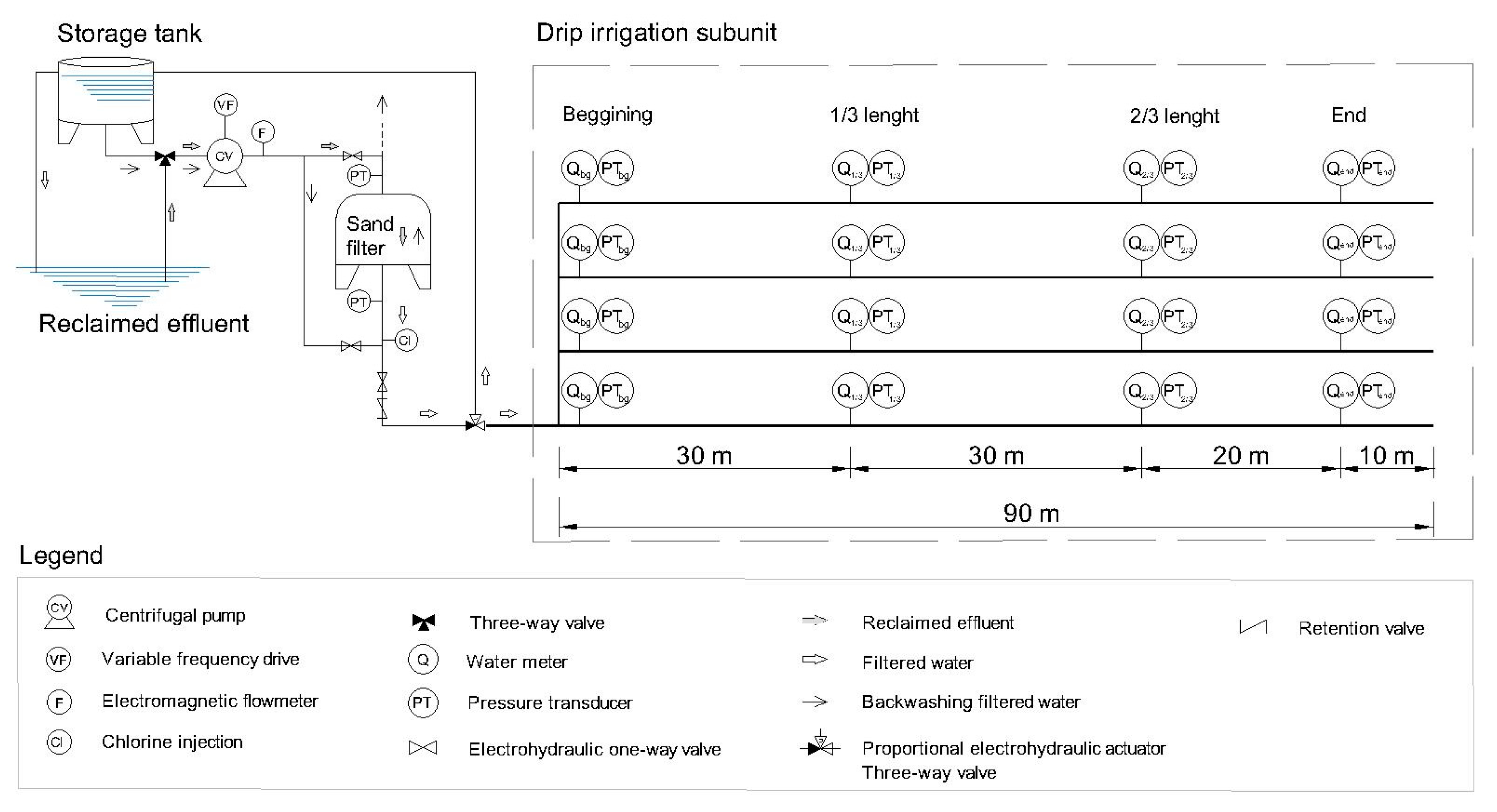
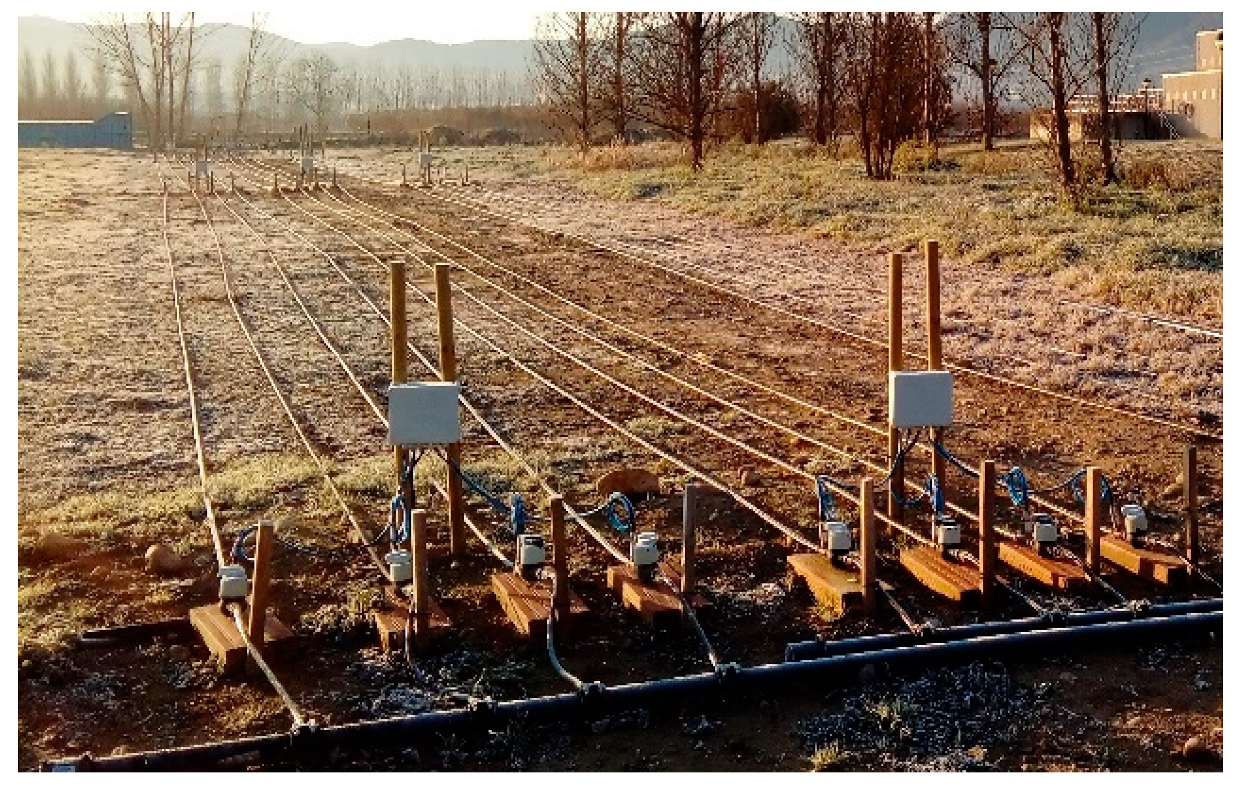
2.1. Experimental Setup

The experiment was carried out using the effluent produced at the wastewater treatment plant (WWTP) of Celrà (Girona, Spain), which treats the urban and industrial wastewaters using an activated sludge process as the secondary treatment. The treated wastewater was pumped into the experimental irrigation system, which consisted of three different irrigation subunits (called A, B, and C, respectively). Each irrigation subunit had a sand filter that differed in its underdrain design. Thus, in one irrigation unit an experimental sand filter built with a porous media underdrain designed by Bové et al. [24] was used, in another a sand filter model FA-F2-188 (Regaber, Parets del Vallès, Spain) was installed, and the third one had a sand filter model FA1M (Lama, Sevilla, Spain). The three sand filters were filled with silica sand of the same characteristics (effective diameter (D_e, size opening which will pass 10% by dry weight of a representative sample of the filter material) of 0.48 mm and coefficient of uniformity (ratio of the size opening which will pass 60% of the sand through the size opening which will pass 10% through) of 1.73). Each irrigation subunit consisted of four laterals with a total length of 90 m each (Figure 1). Commercially integrated and pressure compensating emitters Uniram AS 16010 (Netafim, Tel Aviv, Israel), with 2.3 L/h of nominal flow discharge, a distance between emitters of 0.4 m, a nominal working pressure of 50–400 kPa, and a manufacturing coefficient of variation of 0.03 were used. Driplines had an outside diameter of 16.2 mm and a wall thickness of 1.0 mm. Each lateral had 226 emitters, so there were 904 emitters per irrigation subunit.

2.2. Monitoring Equipment

A multicellular centrifugal pump model CR-15-4 with a rated flow of 12 m³/h and a rated pressure of 500 kPa (Grundfos, Bjerringbro, Denmark) governed by a variable frequency drive model FRN-4 (Fuji Electric, Cerdanyola del Vallès, Spain) pumped the wastewater from the WWTP to the subunits, with the inlet flow measured by an electromagnetic flowmeter Isomag MS2500 (Isoil Industria SpA, Cinisello Balsamo, Italy). Only one irrigation subunit was operating at a time. Since the filtrated flow was higher than that needed for the irrigation subunits, a proportional electrohydraulic actuator SKD32 (Siemens, Munich, Germany) operated a three-way valve VXG41 (Siemens, Munich, Germany), so that the excess flow was brought to a water storage tank of 3000 L Aquablock (Shütz, Selters, Germany) which was used for filter backwashing. The experimental irrigation system also had a chlorine deposit of 200 L in order to continuously inject chlorine to achieve a concentration of 2 mg/L into the effluent after being filtered, using a DosTec AC1/2 membrane pump (ITC, Sta. Perpètua de Mogoda, Spain), aiming to reduce biofilm growth and, consequently, emitter clogging [25]. When sand filters were backwashed, backwashing water entering the filters was chlorinated to reach a 4 mg/L chlorine concentration. The filters were washed automatically when the total pressure drop across them measured by pressure transducers model TM-01/C (Step S.L., Barcelona, Spain), with a measuring operational range from 0 to 600 kPa and an accuracy of ≤±0.5% full scale, reached 50 kPa [8]. The backwashing time was 3 min throughout the test, and during that time, backwashing water did not reach the laterals. The water used for the backwashing came from the filtered water storage tank.

Several effluent quality parameters before and after being filtered were measured and recorded. At filter inlet, electrical conductivity was measured with a transmitter LIQUISYS-M CLM253-CD0010 and a sensor CLS21-C1E4A, and pH and temperature using a transmitter LIQUISYS-M CPM253-MR0010 and a sensor CPS11D-7BA21. At both filter inlet and outlet, turbidity was measured using a transmitter LIQUISYS-M CUM253-TU0005 and a sensor CUS31-A2E, and dissolved oxygen using a transmitter LIQUISYS-M COM253-WX0015 and a sensor COS 61-A1F0. All the transmitters and sensors used were made by Endress + Hauser (Gerlingen, Germany).

Each lateral of each irrigation subunit had water meters and pressure transducers at the beginning, 1/3 of the length, 2/3 of the length, and at the end of the lateral; so there were a total of 16 water meters and 16 pressure transducers for each irrigation subunit (Figure 2). The water meters used were model 405S DN15 (Sensus, Raleigh, NC, USA) with an operational range from 0.3 to 3 m³/h and a precision of ±5% full scale installed with an impulse emitter HRI-A1 (Sensus, Raleigh, NC, USA). This allowed the flow to be calculated in real time. Pressure transducers, model TM-01/C (Step S.L., Barcelona, Spain) with a measuring operational range from 0 to 250 kPa and an accuracy of ±0.5% full scale were used. The water meters and pressure transducers located at the end of the lateral were placed 10 m before the dripline distal end (Figure 1) to ensure that the volume measured was high enough to be within the measurement range.

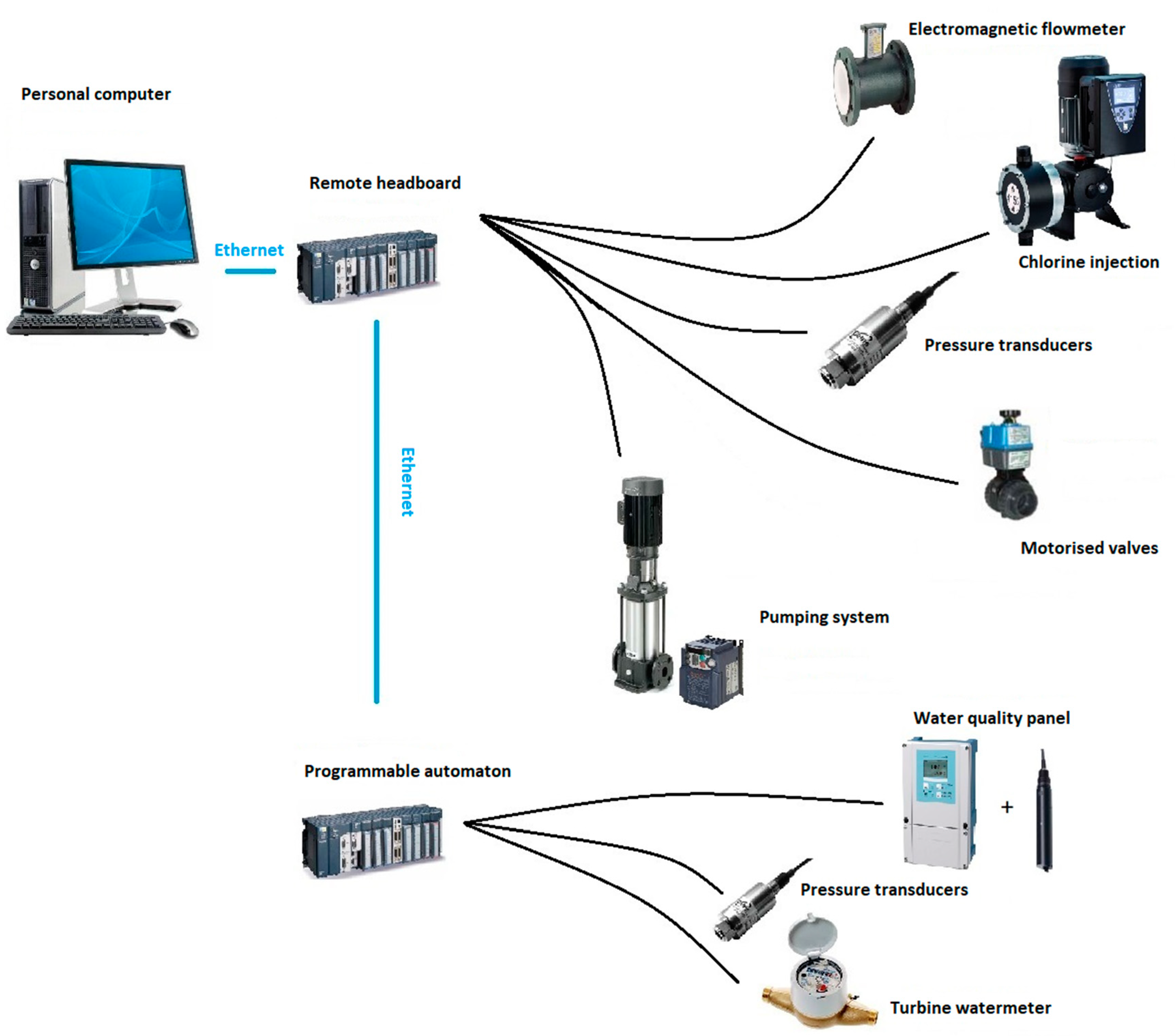
2.3. SCADA System and Components

The SCADA system that was implemented consisted of a personal computer, a programmable automaton, a set of activators and recorders, and a communication network for both of them. All these elements, which allowed measurement of flow and volume, pressure and water quality parameters generated a digital signal or an electric impulse from 4 to 20 mA, which was transformed later to a digital format (16 bits) and stored by a SCADA initially developed by Duran-Ros et al. [26] but was further modified for this experiment.

The personal computer sent data and commands to the programmable automaton and at the same time received data from it. Data were organized, classified, and filed on the computer, which also operated as an interlayer between the user and the installation. The personal computer was an EliteDesk (HP, Palo Alto, CA, USA) with a processer IntelCore I3, with 2.7 GHz and 8 MB de RAM, with an operational system Windows 7 (Microsoft, Redmon, WA, USA). Besides, the computer had the visualization software RSView32 (Rockwell Software, Milwaukee, WI, USA) for the development of human/machine interface.

A programmable automaton, model Compact Logix (Allen-Bradley, Milwaukee, WI, USA) communicated with a remote headboard 1734A (Allen-Bradley, Milwaukee, WI, USA) and accepted orders from the personal computer, to which data were also sent. Communication between devices was via Ethernet (Index protocol) with a 5th category wire. Figure 3 shows the communication network.

Programmable automaton consisted of eight modules with electrical source and input and output modules, and commanded the field automatons:

• Two modules 1769-IQ32 (Allen-Bradley, Milwaukee, WI, USA) with 32 digital inputs each having a direct current of 24 V to detect current flow from lateral water meters and pressure transducers.
• One module 1769-OB16 with 16 digital outputs to activate quality panel valves.
• Three modules 1769-IF16C with 16 analogic inputs with a range of measurement from 4 to 20 mA and a 16-bit resolution, connected to lateral water meters and pressure transducers.
• Two modules 1769-IF4I with four analogic inputs with a range of measurement from 4 to 20 mA and a 16-bit resolution, connected to quality panel transmitters.

Remote headboard ruled the bank filtration automatons and was composed of nine modules:

• Two modules 1734-IB8 with eight digital inputs of direct current of 24 V to detect direct current flow from the four washing triggers of the quality panel, emergency stop, water level sensor of the catch basin, and filtered tank and chlorine tank sensor level.
• Three modules 1734-IEOB8 with eight digital outputs to activate motorized valves and pumping system.
• Three modules 1734-IE8C with eight analogic inputs with a measurable range from 4 to 20 mA and a 16-bit resolution and connected to the headboard flowmeter, quality panel water meters, and to the filter pressure transducers.
• One module 1734-OE4C with four analogic outputs with a measurable range from 4 to 20 mA and a 16-bits resolution connected to the variable frequency drive, headboard centrifugal pump, proportional valve, and the chlorine injection system.

For the automatons that needed electricity supply, two alimentation sources were chosen 1606-XLE-80-E (Alley-Bradley, Milwaukee, WI, USA) which gave 80 W power with 24 V of direct current.

Data from the devices were recorded every minute for the duration of the 1000 h experiment, and could be supervised in real time using the developed human/machine interface. It was also possible to access the personal computer of the experimental setup from any device connected to Internet. For making that possible, a modem model E612 (Huawei, Bantian, China) was installed, with a SIM card (Subscriber Identity Module). By the use of the program Escritorio Movistar (TelefónicaS.A., Madrid, Spain) it was possible to connect to the Internet.

The Internet service hired allocated a variable IP (Internet Protocol) direction. To gain remote access and to be able to control the installation, a TeamViewer program with GPL (General Public License) was used.

2.4. Quality of the Wastewater

Using the monitoring equipment and the SCADA system described in Section 2.3 and Section 2.4, respectively, the main wastewater quality parameters were recorded each minute.

Table 1. Average ± standard deviation of the main physical and chemical parameters of wastewater before and after being filtered. Different letters mean that there were significant differences (p < 0.05) in the values of each parameter.

Subunit	Filter Inlet					Filter Outlet
	pH	Temperature	Electrical Conductivity	Dissolved Oxygen	Turbidity	Dissolved Oxygen	Turbidity
	(-)	(°C)	(dS/m)	(mg/L)	(FTU)	(mg/L)	(FTU)
A	7.33 ± 0.20 b	20.61 ± 3.26 a	2.64 ± 0.46 a	3.27 ± 0.83 b	6.22 ± 2.11	3.31 ± 0.82 b	4.46 ± 1.24 b
B	7.43 ± 0.24 a	20.12 ± 3.49 ab	2.46 ± 0.53 b	3.57 ± 1.02 a	5.82 ± 3.08	3.56 ± 1.04 a	4.18 ± 1.42 c
C	7.31 ± 0.22 b	19.68 ± 3.57 b	2.63 ± 0.44 a	3.28 ± 1.04 b	6.42 ± 2.77	3.25 ± 0.65 b	4.89 ± 1.13 a

shows the mean values of pH, temperature, electrical conductivity, dissolved oxygen, and turbidity during the experiment.

There were significant differences (p < 0.05) for pH, temperature, electrical conductivity, and dissolved oxygen at filter inlets and for dissolved oxygen and turbidity at filter outlet. The variations observed are due to the usual variability in wastewaters. According to Bucks et al. classification [3], the wastewaters pose a moderate chemical clogging hazard and a minor physical clogging hazard.

2.5. Operational Procedure and Data Treatment

The experiment lasted 1000 h for each irrigation subunit, taking place between March and November 2018, and no lateral flushing was carried out during the experiment.

Emitter discharges (observed measures) for all the emitters of all the laterals (i.e., 2712 emitters) were obtained at the beginning, after 500 h and at the end of the experiment (1000 h). In order to measure flow discharge, the volume of each dripper was collected in collection recipients for 5 min and then transferred to a graduated cylinder, with a volume between 100 and 250 mL being collected as recommended by Merriam and Keller [9]. The experimental determination of emitter discharge lasted about 20 h after the target time (0, 500, and 1000 h) due to the number of emitters to be measured. With emitter discharge values for all the emitters in a lateral, the total lateral flow discharge was obtained. In addition, the total water flow at each section of the lateral (Figure 1) was also known.

Following the Merriam and Keller method [9] method, the flow discharge of the two contiguous emitters placed at the beginning, at 1/3, 2/3, and at the end of each lateral length was measured, assuming the mean of the two measurements as representative flow discharge.

Pressure was also determined in these four positions on each lateral during the emitter discharge measurements using a digital manometer Leo 2 (Keller, Winterthur, Switzerland) with a precision of ±0.07% that was placed at a pressure intake (Ein-tal, Or-Akiva, Israel). Distribution uniformity of pressures (DU_lp) [27] was calculated according to the formula:

$$D{U}_{lp}={\left(\frac{p_{25}}{\overline{p}}\right)}^x\times 100$$

(1)

where p₂₅ is the average pressure of 25% of the positions with the lowest pressure (kPa), $\overline{p}$ is the average pressure of all the tested positions (kPa), and x is the emitter flow exponent, which was considered 0.05.

With all emitter flow discharges, flow distribution uniformity (DU_lq) was calculated as:

$$D{U}_{lq}=\frac{q_{25}}{\overline{q}}\times 100$$

(2)

where, q₂₅ is the average flow discharge of 25% of the emitters with the lowest flow discharge (L/h) and $\overline{q}$ is the average flow discharge of all the tested emitters (L/h).

To determine the flow uniformity distribution through the SCADA system, the recorded values during the real measurements of the emitters for each irrigation subunit (at 0 h, 500 h, and 1000 h) were selected. The dripline flow at the beginning, 1/3, and 2/3 lateral length represented the flow of all emitters from the measured point to the end, and the flow at the end represented the flow of the end emitters (last 10 m) (Equation (3)). For that reason, to determine the flow of each lateral stretch, the subsequent measured flow was subtracted from the previous measured flow, following Equations (4)–(6).

q_end = Q_end

(3)

q_2/3 = Q_2/3 − Q_end

(4)

q_1/3 = Q_1/3 − Q_2/3

(5)

q_bg = Q_bg − Q_1/3

(6)

where, Q_end is the measured flow at the last water meter (L/h), Q_2/3 is the measured flow located at 2/3 of the lateral length (L/h), Q_1/3 is the measured flow located at 1/3 of the lateral length (L/h), Q_bg is the measured flow located at the beginning of the lateral (L/h), q_end is the estimated flow of the emitters placed at the end of the lateral (L/h), q_2/3 is the estimated flow of the emitters placed between 2/3 and end water meters (L/h), q_1/3 is the estimated flow of the emitters placed between locations 1/3 and 2/3 of the lateral (L/h), and q_bg is the estimated flow of the emitters placed from the beginning to 1/3 of the lateral (L/h).

Then, the estimated flow for each lateral stretch was divided by the number of emitters in each stretch in order to obtain the average emitter flow discharge for every emitter of each dripline section. So, every lateral had four average emitter discharge values, each of which represented a section, and consequently, every irrigation subunit had sixteen average emitter discharge values. With these values, DU_lq for SCADA system was calculated following Equation (2).

Relative flow was also calculated throughout the experiment as:

$$q_r=\frac{q_h}{q_0}\times 100$$

(7)

where, q_r is the relative flow in a precise time (%), q_h is the flow of a precise time (h) (L/h), and q₀ is the initial flow at 0 h (L/h).

The reduction percentage of relative flow (q_r) and DU_lq with respect to their initial values was calculated as:

$$\mathsf{\Delta }V=\frac{V_0-Vi}{V_0}\times 100$$

(8)

where, ΔV is the reduction percentage (%), V₀ is the initial value, and V_i is the value that needs to be compared.

Mean separation and regression statistical analyses were carried out using SPSS Statistics 25 software (IBM, NY, USA) with a significance level of 0.05.

3. Results and Discussion

3.1. Pressure Distribution across Laterals

Pressure distribution uniformity (DU_lp) values were higher than 98% in all the measurements for all the times (

Table 2. Pressure distribution coefficients (DU_lp, %) of the three irrigation subunits (A, B, and C) at the beginning, after 500 h, and at the end of the experiment measured with the Merriam and Keller [9] and SCADA procedures.

Irrigation Time	0 h			500 h			1000 h			Mean ± Standard Deviation
Subunit	A	B	C	A	B	C	A	B	C
Merriam and Keller (M&K)	98.75	98.66	98.80	98.77	98.27	99.12	99.03	99.04	98.92	98.82 ± 0.26
SCADA	98.94	98.88	98.70	99.00	98.31	99.13	99.13	98.88	98.90	98.88 ± 0.25

). Pressure distribution uniformity values meant that the experimental irrigation system was well designed and, since the emitter manufacturing coefficient of variation was low (3%), discharge reductions can mainly be explained by emitter clogging.

Figure 4 shows the regression between DU_lp calculated in the field using data from the emitters located at those points suggested by Merriam and Keller [9] and that computed using data from pressure transducers located at different driplines points and recorded by the SCADA system. There was a high regression between both methods, with an R² = 0.93 and a signification level of p < 0.01.

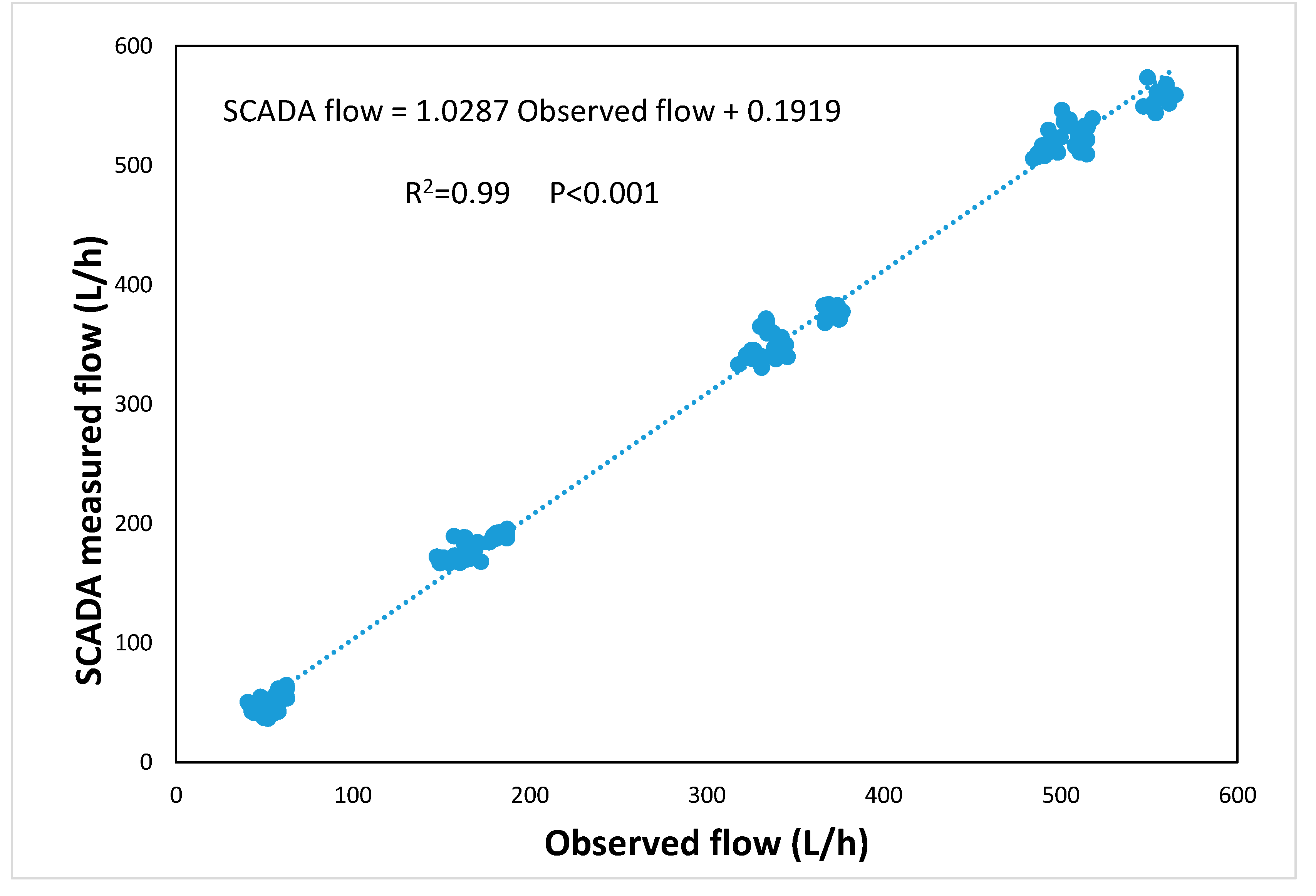
3.2. Measured SCADA Flow Distribution across Laterals

Figure 5 shows the regression between the observed field accumulated emitter discharges and those measured by the SCADA system following the procedure described in Section 2.4. There was a high regression coefficient (R² = 0.99) between the observed flows and the SCADA flows, with a significance level of p < 0.001, which validates that water meter measurements at the dripline and recorded into a SCADA system as a good measurement tool for the real flow of the irrigation subunits for the entire duration of the experiment.

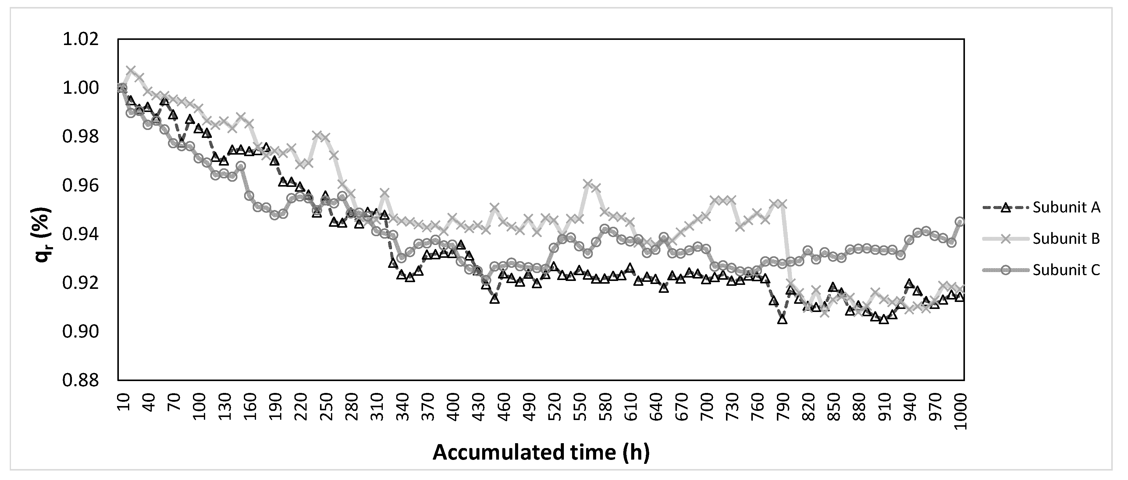
3.3. Dripline Flow Evolution throughout the Experiment

There was a decrease in the flow that went to the irrigation subunits, for all laterals of all subunits with irrigation time. This flow reduction was due to emitter clogging, which commonly happens when low quality waters such as wastewaters, are used in drip irrigation systems [8,13]. Figure 6 shows the average relative flow (q_r), computed following Equation (7) with data of the four water meters placed at the beginning (Q_bg) of each lateral, for each irrigation subunit throughout the experiment. Specific increases in the flow were due to factors such as the switch on and off of the irrigation system, unblocking of the water meters’ protective filters, or emitter discharge variations. For all irrigation subunits, there was a decrease in the q_r along the accumulated irrigation time. The flow decrease was more accentuated from the beginning to 500 h for all irrigation subunits. From 500 h to 750 h of the experiment, q_r of the subunit A remained more or less constant, but it decreased slightly during the last 250 h. A similar behavior was observed for subunit B, where q_r suffered small variation from 500 h to 780 h, but then it suddenly decreased until the end of the experiment. On the other hand, subunit C q_r remained constant for almost all the experiment, with a little increase in the end.

Variation of DU_lq along the experiment can be explained by the flow variation observed in each irrigation subunit. As field DU_lq was measured using data of all emitters at the beginning, after 500 h, and 1000 h, the total flow variation with respect to the initial value of the first water meter was measured as well as DU_lq was computed using Equation (8) (

Table 3. Relative flow (q_r) and relative flow variation (∆q_r), distribution uniformity coefficient (DU_lq) and distribution uniformity coefficient variation (∆DU_lq) at the beginning, after 500, and 1000 h of each irrigation subunit.

Irrigation Subunit	Irrigation Time (h)	qr	Δqr	DUlq	ΔDUlq
A	0	1.00	-	95.41	-
	500	0.92	8.02	92.83	2.70
	1000	0.91	8.58	89.18	6.53
B	0	1.00	-	93.97	-
	500	0.94	5.93	93.07	0.96
	1000	0.92	8.26	87.88	6.48
C	0	1.00	-	96.31	-
	500	0.93	7.40	94.84	1.53
	1000	0.94	6.37	91.44	5.06

). A low correlation between the DU_lq variation (∆DU_lq) and q_r variation (∆q_r) of the first water meter was observed, with an R² = 0.34 but was not significant (p > 0.05). Thus, despite the fact that measuring the whole flow entering in a dripline will be the easiest way for measuring DU_lq, it is not accurate enough to use it, especially when emitter clogging is observed over time. It will be interesting to carry out further research using water meters located at different positions in order to find out if a correlation exists between the flow variation of specific water meters and the DU_lq variation.

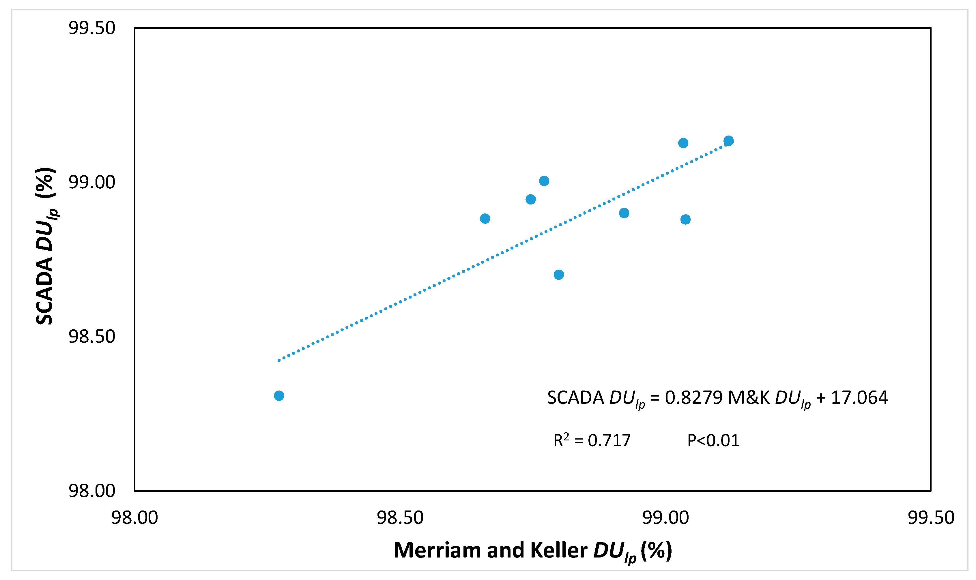
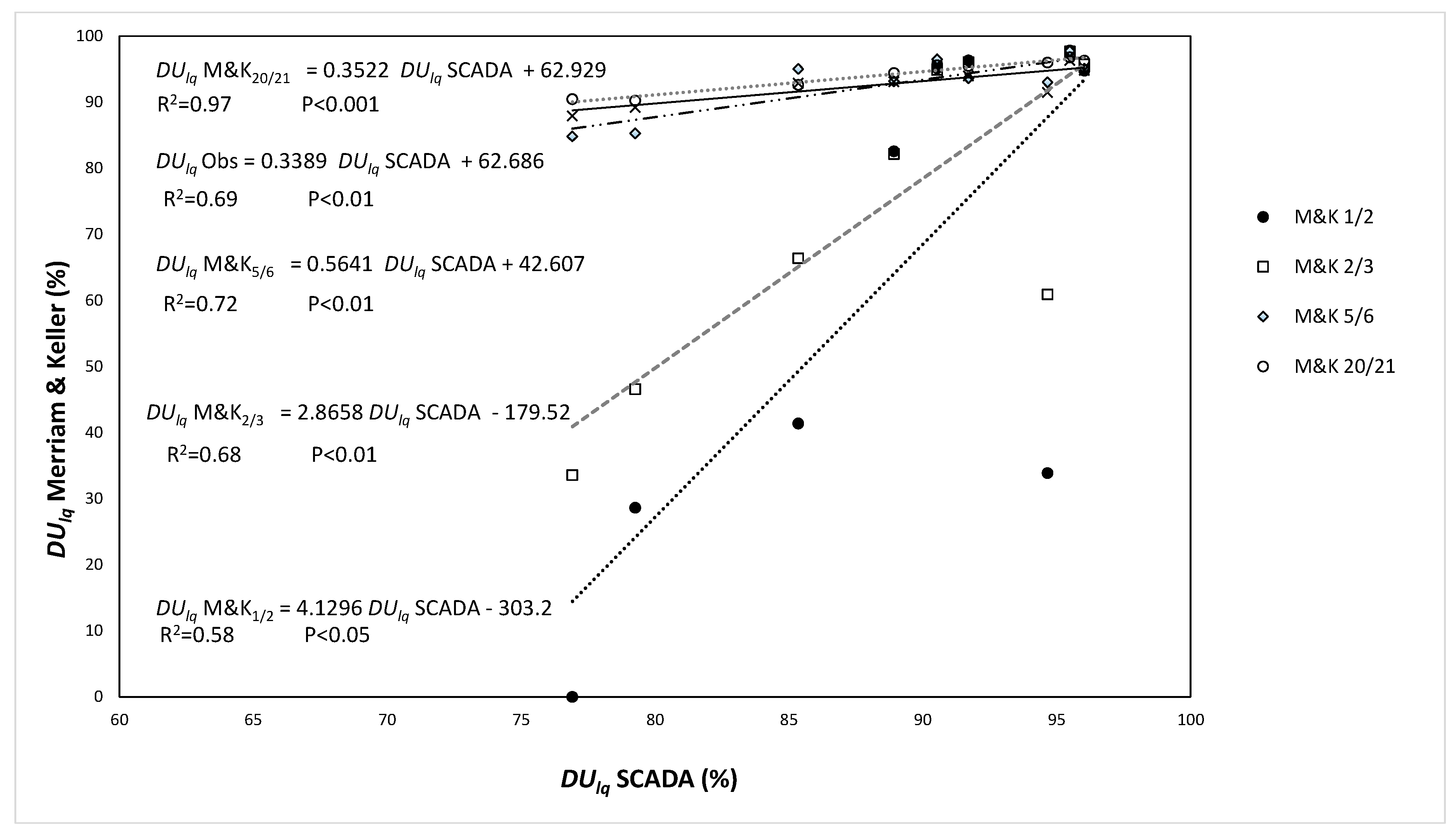
3.4. Comparison of Different Procedures for DU_lq Determination

As Merriam and Keller (M&K) method does not specify which exact emitter location should be used to calculate DU_lq, this index was calculated with different alternative emitter locations at the end of the lateral. Thus, DU_lq was calculated taking the final two emitters (M&K_1/2), the second and third emitters starting from the distal end of the lateral (M&K_2/3), the 5th and 6th (M&K_5/6), and the 20th and 21th (M&K_20/21). The results of the DU_lq are shown in

Table 4. DU_lq calculated for different methods (Merriam and Keller (M&K) observed for all emitters and SCADA) for each irrigation subunit at the beginning, after 500, and 1000 h of the experiment, and its regression significance level with the SCADA method.

	DUlq (%)									p-Value of Regression with SCADA Procedure
Time	0 h			500 h			1000 h
Subunit	A	B	C	A	B	C	A	B	C
M&K1/2	95.15	96.28	97.82	41.37	82.55	94.74	28.61	0.00	33.86	<0.05
M&K2/3	94.85	96.06	97.67	66.36	82.13	95.74	46.57	33.55	60.89	<0.01
M&K5/6	96.49	93.60	97.75	95.02	93.14	95.08	85.29	84.81	92.98	<0.01
M&K20/21	95.57	95.47	96.76	92.62	94.40	96.27	90.23	90.46	95.96	<0.001
Observed	95.41	93.97	96.31	92.83	93.07	94.84	89.18	87.88	91.44	<0.01
SCADA	90.54	91.71	95.50	85.35	88.93	96.03	79.26	76.92	94.66	-

.

Although for the initial stages of the experiment DU_lq did not vary much between the methods, after 500 and especially 1000 h these differences were accentuated, due to a different DU_lq calculation and the effect of emitter clogging. There was a great variation among the DU_lq calculated with different emitter locations following the Merriam and Keller method. Lower DU_lq values were obtained for the emitters of final locations (M&K_1/2 and M&K_2/3) than for the emitters located closer to the beginning of the lateral (M&K_5/6 and M&K_20/21), especially after 1000 h to the experiment, when there is more variability of emitter discharge, mainly due to emitter clogging [7,11]. Merriam and Keller method was penalized due to it taking the emitter discharges of the end of the lateral, although these emitter discharges may not be representative of all emitter discharges of the end section, as end locations are more prone to be partially or completely clogged [12] and affect the DU_lq calculation (Equation (2)). On the other hand, DU_lq obtained with drippers closer to the dripline beginning are higher. This shows which emitter locations should be taken into account when calculating the DU_lq according to Merriam and Keller method, in order to be as representative as possible of the emitter discharges of the irrigation subunit. Merriam and Keller DU_lq adjust more to the observed DU_lq if emitters placed further away from the end are taken into account.

The different DU_lq obtained with the Merriam and Keller method were related with DU_lq obtained with the SCADA system (Figure 7). For the DU_lq taking the last two emitters of the laterals (M&K_1/2), the regression coefficient was low (R² = 0.58), but it increased when other two contiguous emitters were used: R² = 0.68 for M&K_2/3, R² = 0.72 for M&K_5/6, R² = 0.97 for M&K_20/21 and R² = 0.69 for DU_lq obtained with all the observed emitter discharges. Although all regressions were statistically significant, the significance level of M&K_1/2 was lower (p < 0.05) than that for M&K_2/3, M&K_5/6, and Observed (p < 0.01). The regression with SCADA values and M&K_20/21 showed the highest significance level (p < 0.001).

Overall, the SCADA DU_lq had an acceptable correlation to DU_lq measured with all the emitters. A better correlation and better level of significance were observed between SCADA and M&K procedures when this last method took into account the emitters placed closer to the beginning of the lateral. So, DU_lq prediction with SCADA system is a good method of calculation that can replace existing methods such as M&K when measured emitters locations are not those at the very end. In addition, this method would allow the DU_lq monitoring in real time without needing manual field uniformity assessments, with the time and labour cost savings that entails. The proposed system would allow the possibility of determining more frequent DU_lq calculations, having a DU_lq control over time, and would also easily allow subsurface drip irrigation DU calculation. On the other hand, the cost of the instruments and sensors have to be taken into account since investment cost is high and cannot be affordable for some farmers.

4. Conclusions

A supervisory control and data acquisition (SCADA) system allowed to accurately measure the water distribution uniformity in a microirrigation system when using wastewater. Distribution uniformity of pressure and emitter discharges experimentally measured in field conditions showed high regression levels (R² = 0.93 and 0.99, respectively) with data recorded in the SCADA system from pressure transducers and water meters placed at strategic dripline positions. Therefore, SCADA can be used for measuring both pressure and flow discharge of a microirrigation system, which in addition allows monitoring the performance of the irrigation system. The SCADA system will also allow detection of operation anomalies in real time, shortening the time needed for solving them.

SCADA can be a good tool to calculate flow distribution uniformity (DU_lq) of an irrigation system instead of using existing methods such as Merriam and Keller, especially when last emitter locations are not taken into account. Results also showed the incidence of emitter clogging in the DU_lq calculation, and indicate which emitter locations should be measured when determining DU_lq, in order to be representative of the lateral section. Moreover, SCADA will allow calculating DU_lq without the need for annual field measurements, saving labour costs, in spite of its high investment cost.

The proposed method presents automation advantages as it considers indirectly all the irrigation emitters, so DU_lq calculation is as affected by emitter clogging as the Merriam and Keller method. In addition, the proposed method also allows evaluating subsurface irrigation installations that will be impossible to evaluate without digging out the laterals.

References

1. Ayars, J.E.; Bucks, D.A.; Lamm, F.R.; Nakayama, F.S. Introduction. In Microirrigation for Crop Production. Design, Operation and Management; Lamm, F.R., Ayars, J.E., Nakayama, F.S., Eds.; Elsevier: Amsterdam, The Netherlands, 2007; pp. 1–26. [Google Scholar]
2. ICID 2019. Sprinkler and Micro Irrigated Area. Available online: http://www.icid.org/sprinklerandmircro.pdf (accessed on 21 March 2019).
3. Bucks, D.A.; Nakayama, F.S.; Gilbert, R.G. Trickle irrigation water quality and preventive maintenance. Agric. Water Manag. 1979, 2, 149–162. [Google Scholar] [CrossRef]
4. WHO. Guidelines for the Safe Use of Wastewater, Excreta and Greywater; World Health Organization Press: Geneva, Switzerland, 2006; Volume 2. [Google Scholar]
5. Asano, T.; Burton, F.L.; Leverenz, H.L. Water Reuse: Issues, Technologies and Applications; McGraw Hill Inc.: New York, NY, USA, 2007. [Google Scholar]
6. Barragán, J.; Bralts, V.; Wu, I.P. Assessment of emission uniformity for microirrigation design. Biosyst. Eng. 2006, 93, 89–97. [Google Scholar] [CrossRef]
7. Wu, I.P.; Barragán, J.; Bralts, V. Field performance and evaluation. In Microirrigation for Crop Production. Design, Operation and Management; Lamm, F.R., Ayars, J.E., Nakayama, F.S., Eds.; Elsevier: Amsterdam, The Netherlands, 2007; pp. 357–388. [Google Scholar]
8. Ravina, I.; Paz, E.; Sofer, Z.; Marcu, A.; Shisha, A.; Sagi, G. Control of emitter clogging in drip irrigation with reclaimed wastewater. Irrig. Sci. 1992, 13, 129–139. [Google Scholar] [CrossRef]
9. Merriam, J.L.; Keller, J. Farm Irrigation System Evaluation: A Guide for Management; Department of Agricultural and Irrigation Engineering, USU: Logan, UT, USA, 1978. [Google Scholar]
10. Vermeiren, L.; Jobling, G.A. Localized Irrigation; Irrigation and Drainage Paper 36; FAO: Rome, Italy, 1986. [Google Scholar]
11. Juana, L.; Rodríguez-Sinobas, L.; Sánchez, R.; Losada, A. Evaluation of drip irrigation: Selection of emitters and hydraulic characterization of trapezoidal units. Agric. Water Manag. 2007, 90, 13–26. [Google Scholar] [CrossRef]
12. Trooien, T.P.; Lamm, F.R.; Stone, L.R.; Alam, M.; Rogers, D.H.; Clark, G.A.; Schlegel, A.J. Subsurface drip irrigation using livestock wastewater: Dripline flow rates. Appl. Eng. Agric. 2000, 16, 505–508. [Google Scholar] [CrossRef]
13. Puig-Bargués, J.; Arbat, G.; Elbana, M.; Duran-Ros, M.; Barragán, J.; Ramírez de Cartagena, F.; Lamm, F.R. Effect of flushing frequency on emitter clogging in microirrigation with effluents. Agric. Water Manag. 2010, 97, 883–891. [Google Scholar] [CrossRef] [Green Version]
14. Madramootoo, C.A.; Morrison, J. Advances and challenges with micro-irrigation. Irrig. Drain. 2013, 62, 255–261. [Google Scholar] [CrossRef]
15. Goldhamer, D.A.; Fereres, E. Irrigation scheduling of almond trees with trunk diameter sensors. Irrig. Sci. 2004, 23, 11–19. [Google Scholar] [CrossRef]
16. Casadesús, J.; Mata, M.; Marsal, J.; Girona, J. A general algorithm for automated scheduling of drip irrigation in tree crops. Comput. Electron. Agric. 2012, 83, 11–20. [Google Scholar] [CrossRef]
17. González-Perea, R.; Fernández García, I.; Martín Arroyo, M.; Rodríguez Díaz, J.A.; Camacho Poyato, E.; Montesinos, P. Multiplatform application for precision irrigation scheduling in strawberries. Agric. Water Manag. 2017, 183, 194–201. [Google Scholar] [CrossRef]
18. Morillo, J.G.; Martín, M.; Camacho, E.; Rodríguez Díaz, J.A.; Montesinos, P. Toward precision irrigation for intensive strawberry cultivation. Agric. Water Manag. 2015, 151, 43–51. [Google Scholar] [CrossRef]
19. Sivagami, A.; Hareeshvare, U.; Maheshwar, S.; Venkatachalapathy, V.S.K. Automated irrigation system for greenhouse monitoring. J. Inst. Eng. Ser. A 2018, 99, 183–191. [Google Scholar] [CrossRef]
20. Fernández-Pacheco, D.G.; Molina-Martínez, J.M.; Jiménez, M.; Pagán, F.J.; Ruiz-Canales, A. SCADA platform for regulated deficit irrigation management of almond trees. J. Irrig. Drain. Eng. 2014, 140, 04014008. [Google Scholar] [CrossRef]
21. Li, D.; Hendricks Franssen, H.-J.; Han, X.; Jiménez-Bello, M.A.; Martínez Alzamora, F.; Vereecken, H. Evaluation of an operational real-time irrigation scheduling scheme for drip irrigated citrus fields in Picassent, Spain. Agric. Water Manag. 2018, 208, 465–477. [Google Scholar] [CrossRef] [Green Version]
22. Rijo, M. Design and field tuning of an upstream controlled canal network SCADA. Irrig. Drain. 2008, 57, 123–137. [Google Scholar] [CrossRef] [Green Version]
23. Rijo, M.; Arranja, C. Supervision and water depth automatic control of an irrigation canal. J. Irrig. Drain. Eng. 2010, 136, 3–10. [Google Scholar] [CrossRef]
24. Bové, J.; Puig-Bargués, J.; Arbat, G.; Duran-Ros, M.; Pujol, T.; Pujol, J.; Ramírez de Cartagena, F. Development of a new underdrain for improving the efficiency of microirrigation sand media filters. Agric. Water Manag. 2017, 179, 296–305. [Google Scholar] [CrossRef]
25. Li, J.; Chen, L.; Li, Y.; Yin, J.; Zhang, H. Effects of chlorination schemes on clogging in drip emitters during application of sewage effluent. Appl. Eng. Agric. 2010, 26, 565–578. [Google Scholar] [CrossRef]
26. Duran-Ros, M.; Puig-Bargués, J.; Arbat, G.; Barragán, J.; Ramírez de Cartagena, F. Definition of a SCADA system for a microirrigation network with effluents. Comput. Electron. Agric. 2008, 64, 338–342. [Google Scholar] [CrossRef]
27. Bliesner, R.D. Field evaluation of trickle irrigation efficiency. In Proceedings of the ASCE Irrigation and Drainage Division Specialty Conference on Water Management for Irrigation and Drainage, Reno, NV, USA, 20–22 July 1977; pp. 382–393. [Google Scholar]
Figure 1. Diagram of the experimental irrigation system. For simplicity, only one out of the three drip irrigation subunits is depicted.
Water 11 01346 g001
Figure 2. View of the pressure transducers and water meters of the irrigation subunits.
Water 11 01346 g002
Figure 3. Communication network of the supervisory control and data acquisition (SCADA) system developed.
Water 11 01346 g003
Figure 4. Relationship between observed DUlp (%) following Merriam and Keller procedure and DUlp (%) recorded by the SCADA system at the beginning, after 500 h, and 1000 h of the experiment.
Water 11 01346 g004
Figure 5. Relationship between the observed flow (L/h) and the measured flow by the SCADA system (L/h) for all water meters at different locations and measuring times.
Water 11 01346 g005
Figure 6. Average relative flow of the four water meters placed at the beginning for each irrigation subunit along the 1000 h experiment.
Water 11 01346 g006
Figure 7. Relationship between DUlq SCADA and DUlq using Merriam and Keller method taking different end emitters, and DUlq for all emitters (Observed).
Water 11 01346 g007