Article

Parsimonious Modeling of Snow Accumulation and Snowmelt Processes in High Mountain Basins

1
Departamento de Ingeniería Geomática e Hidráulica, Universidad de Guanajuato, Av. Juárez 77, Zona Centro, Guanajuato 36000, México
2
Research Institute of Water Engineering and Environment, Universitat Politècnica de València, Camino de Vera s/n, 46022 Valencia, Spain
*
Author to whom correspondence should be addressed.
Water 2019, 11(6), 1288; https://doi.org/10.3390/w11061288
Submission received: 16 March 2019 / Revised: 9 June 2019 / Accepted: 10 June 2019 / Published: 20 June 2019

Abstract

:
The success of hydrological modeling of a high mountain basin depends in most case on the accurate quantification of the snowmelt. However, mathematically modeling snowmelt is not a simple task due to, on one hand, the high number of variables that can be relevant and can change significantly in space and, in the other hand, the low availability of most of them in practical engineering. Therefore, this research proposes to modify the original equation of the classical degree-day model to introduce the spatial and temporal variability of the degree-day factor. To evaluate the effects of the variability in the hydrological modeling and the snowmelt modeling at the cell and hillslope scale. We propose to introduce the spatial and temporal variability of the degree-day factor using maps of radiation indices. These maps consider the position of the sun according to the time of year, solar radiation, insolation, topography and shaded-relief topography. Our priority has been to keep the parsimony of the snowmelt model that can be implemented in high mountain basins with limited observed input. The snowmelt model was included as a new module in the TETIS distributed hydrological model. The results show significant improvements in hydrological modeling in the spring period when the snowmelt is more important. At cell and hillslope scale errors are diminished in the snowpack, improving the representation of the flows and storages that intervene in high mountain basins.

1. Introduction

The success of hydrologic modeling of high mountain basins depends in most cases on the correct quantification of snow accumulation and melting processes. According to [1], snow accumulation in winter as well as spring snowmelt gives to mountain catchments a particular hydrological response that should be taken into account when modeling river runoff. Also, mountain catchments are very sensible to temperature changes; therefore climate change can drastically impact the hydrological cycle [2,3]. For example, snowmelt is one of the processes intervening in the hydrological cycle and interacting with many other processes [4]. According to [5], climate change is likely to impact the seasonality and generation processes of floods, which has direct implications for flood risk assessment, design flood estimation, and hydropower production management. Therefore, it is very evident the importance of modeling the accumulation and snowmelt in mountain basins where a very high percentage of water comes from snow [4]. However, mathematically modeling of these processes is not an easy task due to the high spatial and temporal variability of the snow accumulation by itself and strong relationship of snowmelting and with precipitation, temperature, and orographic effects [6,7]. The study their relationship with runoff coming from snowmelt is a recent and recurrent topic [8,9,10]. These processes and relationships are traditionally modeled with mathematical simplifications that are based on simple approaches such as degree-day models and more complex conceptualizations such as energy balance models [11]. These mathematical simplifications are generally implemented as modules executed in hydrological conceptual rainfall-runoff models. There are recent publications that use models developed to implement the snow-runoff process (i.e., [12,13,14,15]).
Unfortunately, the use of energy balance models is not the practical solution due to the high number of variables that can be relevant and can change significantly in space and, in the other hand, the low availability of most of them in a typical [16]. In addition, if used, most of the needed variables are indirectly estimated that increase the uncertainty in the results [16]. For the above mentioned reasons, we decided to the degree-day approach as an option for mountain catchments with limited observed input. According to [17] the classical degree-day model is the conceptualization most used for its parsimony and easy application in medium and large basins. Use only temperature and a spatially constant parameter denominated degree-day factor in their formulation, comprise one of these simplifications. However, according to Hock [18], these models incorrectly reproduce the spatial variability of the snowmelt, because the degree-day factor actually changes in time and space due to the influence of a series of variables such as: season, ground cover, topography, snow cover, snow contamination, atmospheric conditions and rainfall. Consequently, in recent decades there has been an attempt to introduce the variability of the degree-day factor using hybrid mathematical formulations that consider the distribution of the energy flow of longwave radiation (LWR) and shortwave radiation (SWR) as those proposed by [6,18,19,20,21]. Nevertheless, Hock [22] pointed out that there are two problems when using the distributed degree-day model: (a) despite working with long time periods, its precision diminishes when the temporal resolution increases and; (b) the spatial variability is not modeled with precision, because the snowmelt rates can vary substantially influenced by topographic effects such as hill shade, slope and orientation.
For these reasons, our research introduces the spatial and temporal variability of the degree-day factor, using a new modification of the equation of the classical degree-day method with different approaches that will be compared. Moreover, we evaluate the effects of the variability in the hydrological modeling and the snowmelt modeling at the cell and slope scale in two high mountain basins. In this research, we decided to implement the new snowmelt formulation in the distributed hydrological model TETIS, with physically-based parameters developed by the Research Group of Hydrological and Environmental Modeling of the Polytechnic University of Valencia, Spain. The TETIS model simulates the main processes of the hydrological cycle through a conceptualization of tanks [23]. The TETIS model is a free software available at http://lluvia.dihma.upv.es/ES/software/software.html. This model has been implemented in a high number of basins in Spain [24] and Latin America [25], and also there are applications in France [26], USA [27], UK [28], and China [29].

2. Case Studies

The basins selected for the case studies in this paper are the Carson River and the American River basins located in the Sierra Nevada, between the states of California and Nevada in the United States (longitude 118 –124 W and latitude 38 –40 N) (Figure 1). These two basins have also been used in the Distributed Hydrologic Model Intercomparison Project-Phase 2 (DMIP2) directed by the National Weather Service of the National Oceanic and Atmospheric Administration [30].
Despite being geographically quite close, the hydrologic regimes of these basins are very different due to the average elevation and the location of the dividing line of the Sierra Nevada [31]. The Carson River basin has an area of 922 km 2 and is has an altitude of between 1548 m and 3408 m. This basin presents a hydrologic regime completely dominated by snow. The American River basin has an area of 886 km 2 and has a lower altitude than that of the Carson, between 281 m and 2630 m. The hydrologic regime of this basin is mixed, influenced by rain and snow. According to NFDC1, GRDN2, and CMEC1 streamflow gauges (Figure 1), the most important runoffs in the basins are registered in spring and summer. The Carson River basin registers a mean annual accumulated precipitation of between 559 mm and 1244 mm, and the American River basin records a mean annual accumulated precipitation of between 813 mm and 1651 mm [32]. Furthermore, the mean annual temperature of the Carson River basin varies between 0 C to 14 C, while that of the American River basin is between 3 C and 18 C [32].

3. Methodology

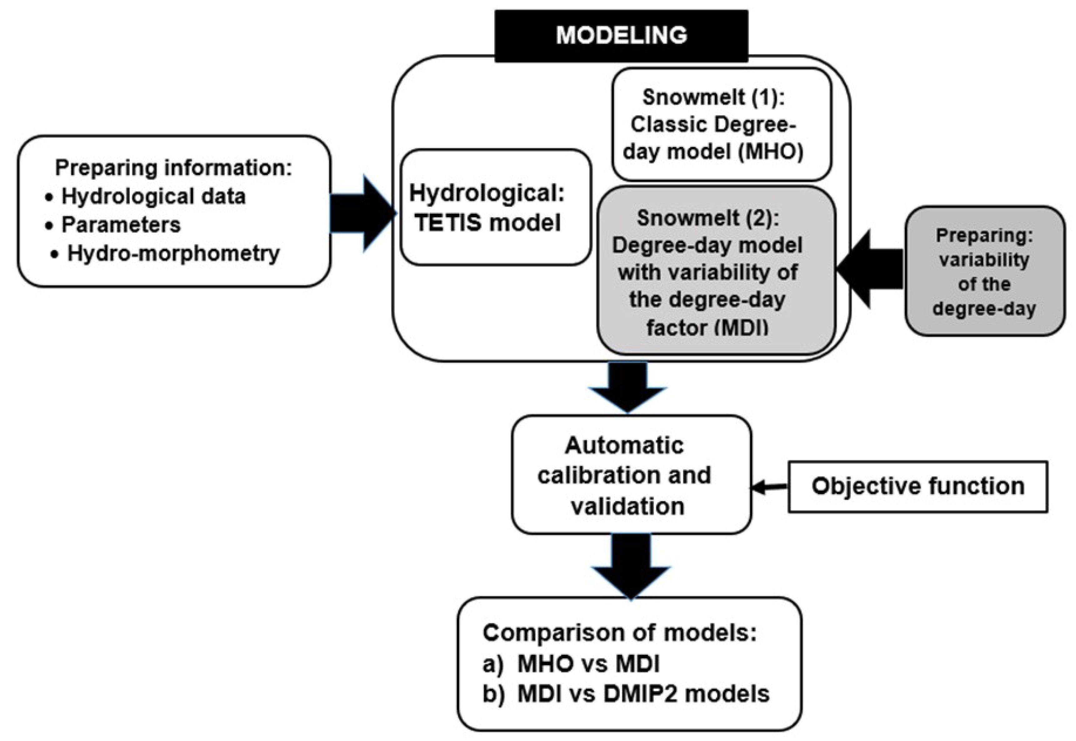
To perform a better hydrological and snowmelt modeling of high mountain basins with limited observed input, this paper proposes a methodology that consists of several phases (Figure 2). In hydrological modeling we use the TETIS model, which is a conceptual model with physically-based parameters [23]. The TETIS model is described in detail later. On the other hand, in snowmelt modeling we use the degree-day method. This method has shown good results in a high number of basins which vary in size [33] and is widely used because it requires little information and it is easily adaptable to rainfall-runoff models. The choice of this method is basically due to the shortage of complete information of net radiation, sensible energy, latent energy, soil heat and energy advection. This information is necessary to estimate the snowmelt using the models which consider the energy balance applying the conservation laws [34].
For the foregoing, we propose a modification to the original equation of the degree-day model, to introduce the variability of the degree-day factor. The models are automatically calibrated and are compared with the models of the Distributed Hydrologic Model Intercomparison Project-Phase 2 (DMIP2), of the National Weather Service (NWS) of the National Oceanic and Atmospheric Administration (NOAA) [30].
The information and data used in the modeling have been obtained from the database of the DMIP2. This information is available to the public at the following link http://www.nws.noaa.gov/oh/hrl/dmip/2. The database of DMIP2 includes a Digital Elevation Model (DEM), soils and vegetation data, which are used to perform the basin characterization and calculation of TETIS model parameters. In addition, the hourly observed precipitation data, temperature, streamflow, daily snow water equivalent and snow cover data were used as inputs in the calibration and validation of the models. In the hydrologic modeling of these basins, hourly precipitation and temperatures and instantaneous hourly streamflow data have been used. For more information about this hydro-meteorological information you can consult [30]. The modeling has also used monthly potential evapotranspiration data, daily Snow Water Equivalent data (SWE) and a total of 254 satellite images of snowpack provided by NWS of NOAA, used to validate the spatial distribution of mathematically simulated snowpack.

3.1. Hydrological Model

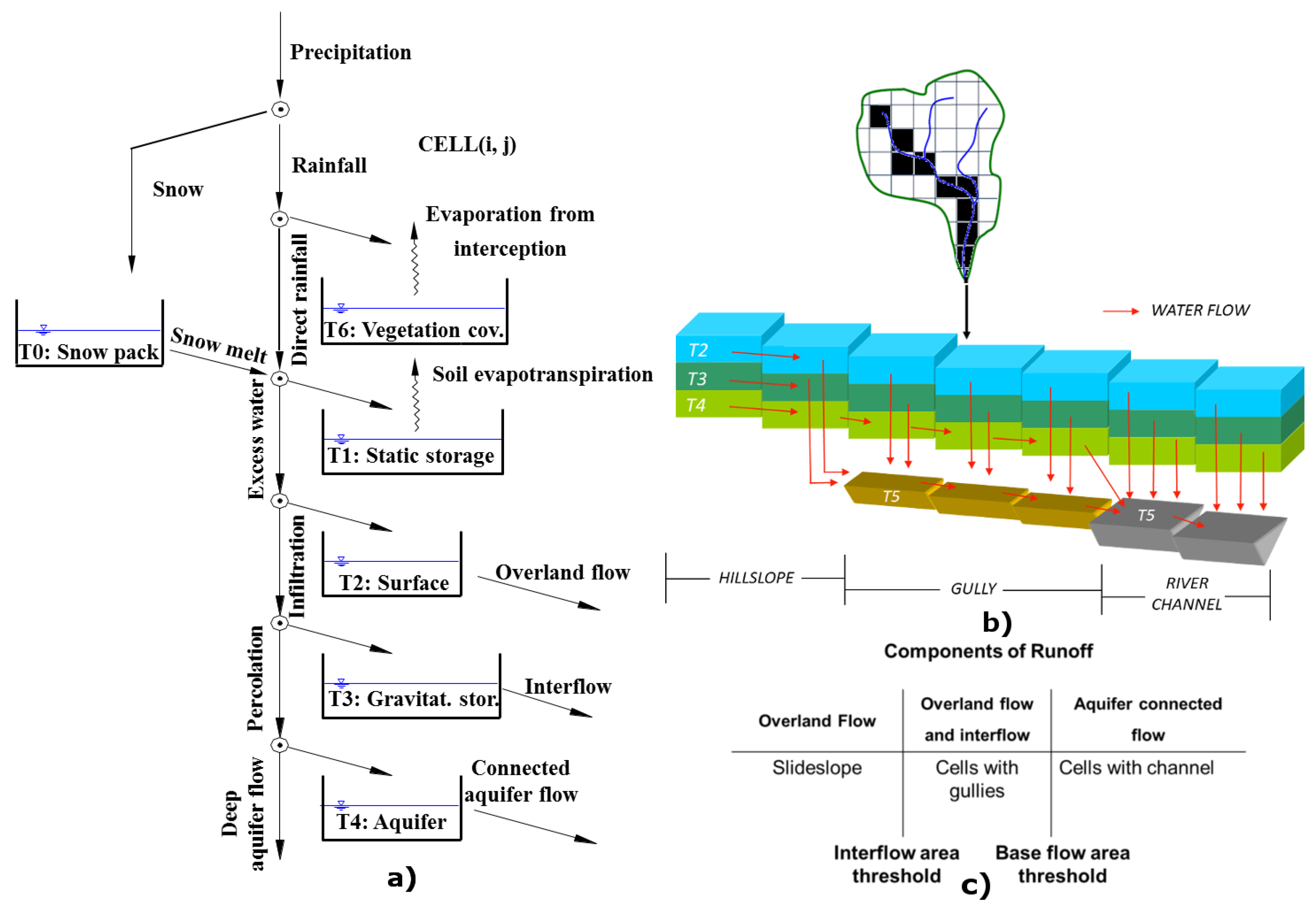
The TETIS model represents the main processes of the hydrological cycle at different spatial and temporal scales, besides water storage and vertical movement on the slopes, in the riverbeds, and the aquifer (Figure 3). In its conceptual scheme, the vertical flow of water is distributed in six levels or tanks where runoff production and state variables are obtained by a simple hydrological balance in each cell (Figure 3a). The horizontal flow of the water is carried out laterally considering three outcomes: direct runoff, interflow and base flow (Figure 3b). These flows follow the flow directions until they reach the drainage network constituted by gullies and streambeds.
The propagation of the flows in the streambed networks is modeled using the so-called Geomorphological Kinematic Wave which is a simplification of the Saint Venant equations as it disregards inertial and pressure terms. To differentiate the aforementioned flow components, the TETIS model uses threshold areas. For example, when the interflow of a cell where the area drained is superior to the threshold area, the flow becomes superficial and flows through gullies (Figure 3c).

3.2. Snowmelt Model

In snowmelt modeling, the original TETIS model uses the classic degree-day method with homogeneous parameters. This model will be used to evaluate and differentiate the effects of the variability of the degree-day factor in the hydrological and snowmelt modeling. The degree-day snowmelt model with homogeneous parameters (MHO) uses a snow tank ( T 0 ) in the conceptual scheme of the TETIS model (Figure 3). T 0 tank holds the solid precipitation (i.e., snow) differentiates from liquid precipitation using a base temperature. The snowmelt runoff stored in the T 0 tank is quantified using the following equation:
M ( i ) = D D F 1 , 2 T a ( i ) T b , if T a ( i ) T b and S W E > 0 0 , if T a ( i ) < T b
where M ( i ) is the snowmelt runoff in each cell (mmd 1 ), D D F 1 is the homogeneous degree-day factor (mm C 1 d 1 ) which this model uses when there is no rain, D D F 2 is the degree-day factor, also homogeneous, that the model uses when there is energy input from rain (mm C 1 d 1 ), T a ( i ) is the mean air temperature in each cell (°C) and T b is the base temperature (°C). This model also uses a threshold temperature to differentiate solid from liquid precipitation, which usually is T b . The inputs that the MHO model requires are precipitation and mean air temperature data. The snowmelt rates and SWE in each cell are the outputs given.

4. Spatio-Temporal Variability of the Degree-Day Factor

Our proposed mathematical formulation of snowmelt, identified as MDI, was designed taking into account the models developed by [6,18,19,21,35,36,37,38]. In particular, our proposal conserves the parsimony of the classic model described previously (i.e., it can be used in basins with limited observed input), but introduces the spatial and temporal variability of the degree-day factor using maps of relative radiation indices. We decided to use shortwave radiation (SWR) because according to Kustas et al. [19], this radiation better explains the variability of the snowmelt process. In addition, Ohmura et al. [39] identify shortwave radiation as the greatest source of energy for snowmelt. Therefore, our snowmelt model is different from previous ones, because it considers the spatial (scale of cell) and temporal (monthly) distribution of degree-day factor considering the position of the sun and the topography. The formulation that the MDI model uses is the following:
M ( i ) = M f 1 , 2 · I R ( i ) T a ( i ) T b , if T a ( i ) T b and S W E > 0 0 , if T a ( i ) < T b
where M f 1 is the degree-day factor (mm C 1 d 1 ) to be affected in space by I R , M f 2 factor for rainy days (mm C 1 d 1 ) , T a ( i ) is the mean air temperature in each cell (°C) at time i, T b is the base temperature (°C) and I R ( i ) is a dimensionless coefficient for time of the year i that introduces the energy values of shortwave radiation actually received in each cell compared with the values of shortwave radiation received on a flat surface:
I R ( i ) = S W R v ( i ) S W R h ( i )
where S W R v is shortwave potential radiation (Whm 2 ) calculated considering the slope, orientation, relief shading and the zenith angle depending on the time of the year; S W R h is shortwave potential radiation received on a flat surface at the same altitude and time of the year (Whm 2 ). To calculate SWR, a DEM of 400 m resolution and the script Area Solar Radiation of ArcGIS, which uses the Viewshed algorithm developed by [40] and modified by [41], was applied.
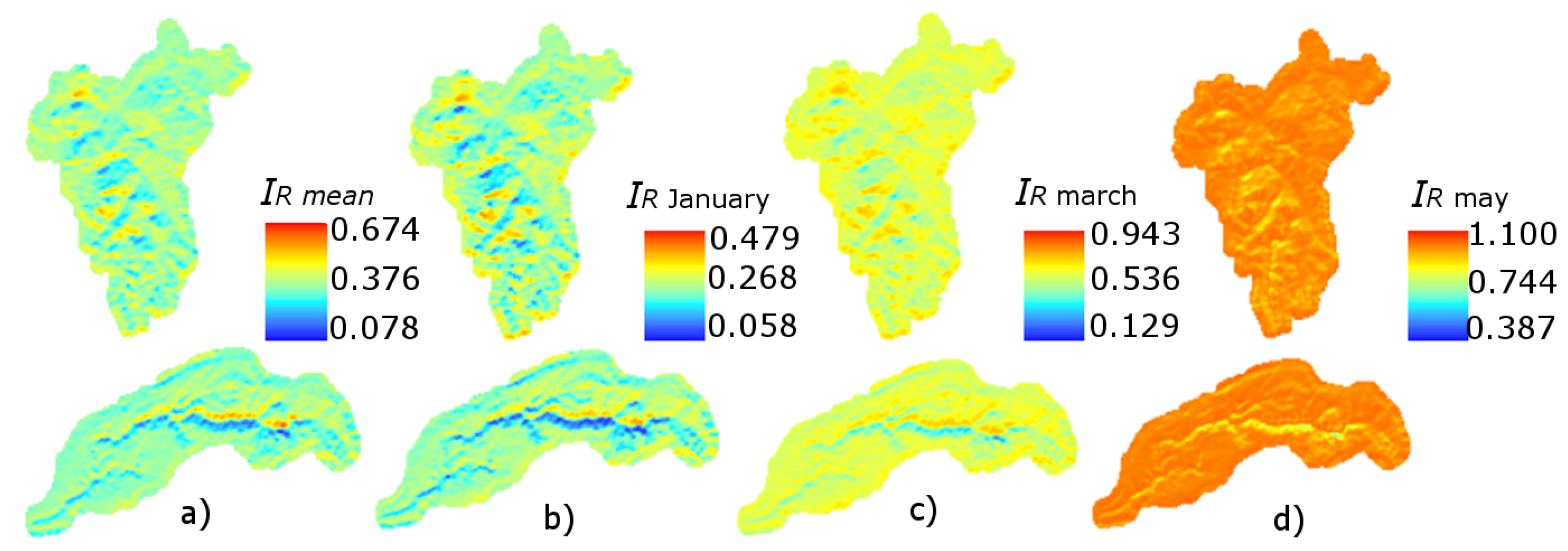
Actually, the MDI model has been evaluated in two modalities: (i) MDI-1, using a single I R map computed as the mean annual value, and (ii) MDI-6, using six monthly I R ( i ) maps, calculated for the months from January to July, and applied by symmetry to each month of the year. In Figure 4, there are some examples of the I R maps obtained for both basins. The I R calculated for each cell from the SWR are introduced into the model by maps of the radiation indices in ascii format.

5. Calibration and Validation of Models

The hydrologic and snowmelt models have been calibrated automatically employing the optimization algorithm Shuffled Complex Evolution of the University of Arizona (SCE-UA) proposed by [42,43]. The decision to use the SCE-UA has to do with its popularity, being employed by various hydrologic models, such as the SAC-SMA [44], the NWSRFS-SMA [45], the MIKE11/NAM [46] and many others, but mainly because it works perfectly with the effective parameters of the TETIS [23]. Also, automatic calibration allows a fairer comparison between different models. The methodology followed in this research consists of a combined automatic calibration, that is, the parameters of the hydrologic model TETIS and the parameters of the MHO and MDI models have been calibrated together. Table 1 shows the parameters of the TETIS model calibrated by correction factors (FC) which make a global correction of the initial parameters quantified with the information available [23]. Table 2 shows the parameters of the snowmelt models calibrated automatically with the SCE-UA.
In the evaluation of the results obtained with the hydrological model and the different alternatives for snowmelt models, we use the Nash-Sutcliffe Efficiency index (NSE) as an objective function. This index is commonly used as a measure of efficiency in hydrologic models given that it involves the standardization of the residual variance and its expected value does not change with the length of the record [47,48,49,50]. The NSE contemplates efficiency between and 1, one being the perfect adjustment between the observed flow and the simulated flow. In scientific literature, a calibration is acceptable when the NSE value is higher than 0.6 and excellent when the NSE value is higher than 0.8 [51]. The NSE calculation has been carried out using the following equation:
N S E = 1 i = 1 n q o b s ( i ) q s i m ( i ) 2 i = 1 n q o b s ( i ) q ¯ o b s ( i ) 2
where q o b s is the observed flow, q s i m the simulated flow and q ¯ o b s is the mean flow observed.
The calibration consisted of a warm up of a water year from which the initial moisture conditions and state variables used in basin modeling are obtained (Table 3). The calibration period selected consisted of two water years, one wet and one dry, the former, with the objective of obtaining effective parameters that were robust and capable of representing these variations in annual events. We decided to use a short period of two years to reduce the computation times employed in the optimization, which when combined with a separated structure of effective parameters of the model can be sufficient.
The predictive capacity of the models in was evaluated through spatial, temporal and spatio-temporal validation (Table 3). In the validation of the snowmelt models implemented, six SNOTEL stations have been used (Figure 1): Blue Lakes, Ebbetts Pass, Poison Flats, Spratt Creek, Blue Canyon and Huysink.
In the evaluation and analysis of the results obtained with the different alternatives for snowmelt models, they have been: the Root of Mean Square Error (RMSE) and the SWE Centroid Date (SCD) has been used as in other studies such as by [52].
The RMSE is widely used and it is computed using the following equation:
R M S E = i = 1 n q o b s ( i ) q s i m ( i ) 2 n 1 / 2
where n is the number of observations.
The SCD is computed using the following equation:
S C D = t i x S W E i S W E i
where S W E is the daily observed or simulated S W E in mm, t is the number of the day from the beginning of snow accumulation and i denotes an individual S W E value.
Finally, simulated snowpacks were validated with a total of 202 satellite images at a resolution of 1 km. Obtaining the differences between the area of the simulated snowpacks and the area obtained from satellite images in percent. Moreover, the DDF variability effects in the hillside snow modeling use a set of cells located on the northern and southern hillsides was selected.

6. Results and Discussion

The first analysis carried out consisted of comparing the effective parameters of the hydrological models obtained with the SCE-UA algorithm. The effective parameters in both basins show significant differences, because the state variables and the flows in each cell have different results influenced by the hydrological regime of these basins (Table 4).
Nonetheless, as can be observed in Table 4, the effective parameters of the snowmelt models do present significant differences directly related to the spatial and temporal variability of the I R used in each case (Figure 5). Table 4 also demonstrate that in both basins, the MDI-6 model has obtained minimum DDFs and is lower than the fixed range of 1 to 11.6 mm C 1 d 1 , taking into consideration the results of [22,53,54]. Also, a greater variability is achieved for both basins when six I R maps are used and follows a pattern clearly influenced by the orientation of the hillside, the relief shading, and the zenith angle. The former coincides with that stated by [22] who considers it fundamental to introduce the effect of these variables in the DDF, which has been achieved with this new snowmelt model.
On carrying out the sensitivity analysis of the MDI-1 and MDI-6 models to the D D F 1 and D D F 2 parameters, it was observed that both snowmelt models are not very sensitive to the D D F 2 , because the condition that combines rainfall and air temperatures is higher than the base temperature that activates the snowmelt mechanism and is not representative. Greater sensitivity was observed in the snowmelt models for the D D F 1 factor.

6.1. Rainfall-Runoff Modeling

The efficiencies obtained in the flow modeling observed in the calibration period has demonstrated that in both basins the DDF variability significantly influences the quantification of the flows at the streamflow gauges. On analyzing separately the efficiencies of a wet year and a dry year, it was observed that there are important differences in the snowmelt models. In Table 5, it can be observed that the MHO obtained high efficiencies for the wet period and worse results for the dry year in both basins. In the same tables, it can be seen that the MDI-1 also obtained worse results in the dry period, improving its efficiencies in the wet period. The MDI-6 model obtained very good efficiencies in the wet period and the best results in the dry period.
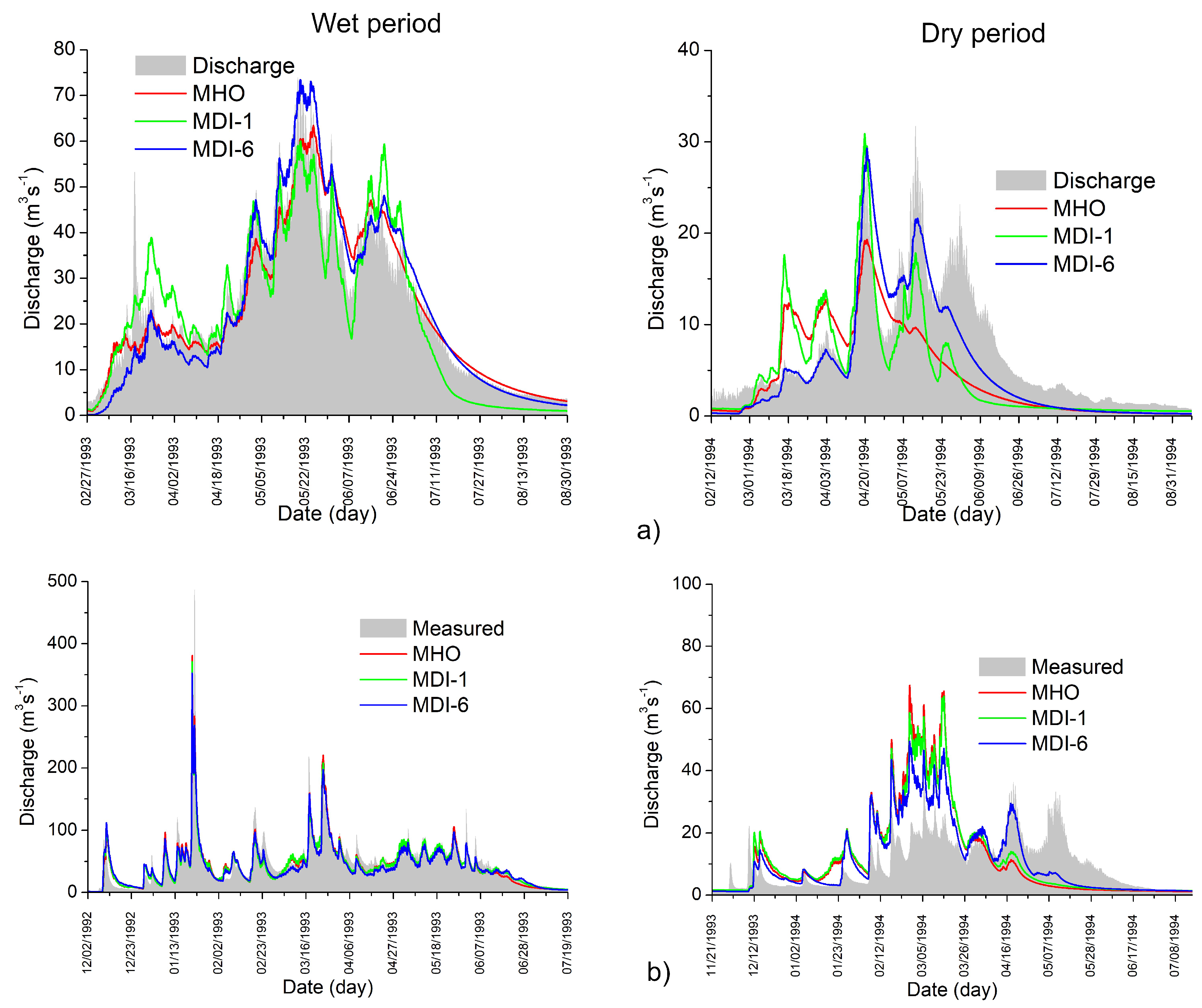
In Figure 6 we can better observe the effect of the day-grade factor on overestimations of the snowmelt, which produce large contributions to the melt flow in winter and decrease considerably in the spring thaw. Although the differences do not seem so significant, it can be seen that the MDI-6 model approaches better to the recession curve of the observed hydrograph (Figure 6). This indicates that introducing the variability of the degree-day factor allows a better approximation to the real snowmelt rates. The opposite case is observed in the models MDI-1 and MHO, where the rates are too high, causing a faster snowmelt even in winter months. This is more evident in the drought period, where the sensitivity of using homogeneous degree-day factor produces very large errors in hydrological modeling (Table 5).
The predictive capacity of the models evaluated by temporal, spatial and spatio-temporal validation is in the range of those achieved by the DMIP2 model [30]. The efficiencies in the temporal validation show that MDI-6 is the model that achieves the best prediction in both basins (Table 6). In the case of the spatial validation, again the MDI-6 is the model that obtained the best efficiencies in the Carson River basin. In the spatio-temporal validation, the results show the best efficiencies distributed between the two models. In general, the MDI models show a prediction of between acceptable and very good where the effect of variability in the modeling of the flows observed is positive with respect to the MHO model.
In continuous simulations (Table 6), the efficiencies of the MDI-6 are also better and of the order of those obtained by models: HL-RDHM [55], NWSRFS [43], TOPKAPI [56] and GR4J [45] in the same basin (Table 7).

6.2. Modeling Snow Accumulation and Snowmelt

In snow modeling, the point accumulation of the snow is evaluated using daily SWE data from four SNOTEL stations located in the Carson River basin and two in the American River basin. The efficiencies achieved in the calibration period have shown that the models obtained the best results in the SNOTEL stations located at an altitude higher than 2000 m (Table 8).
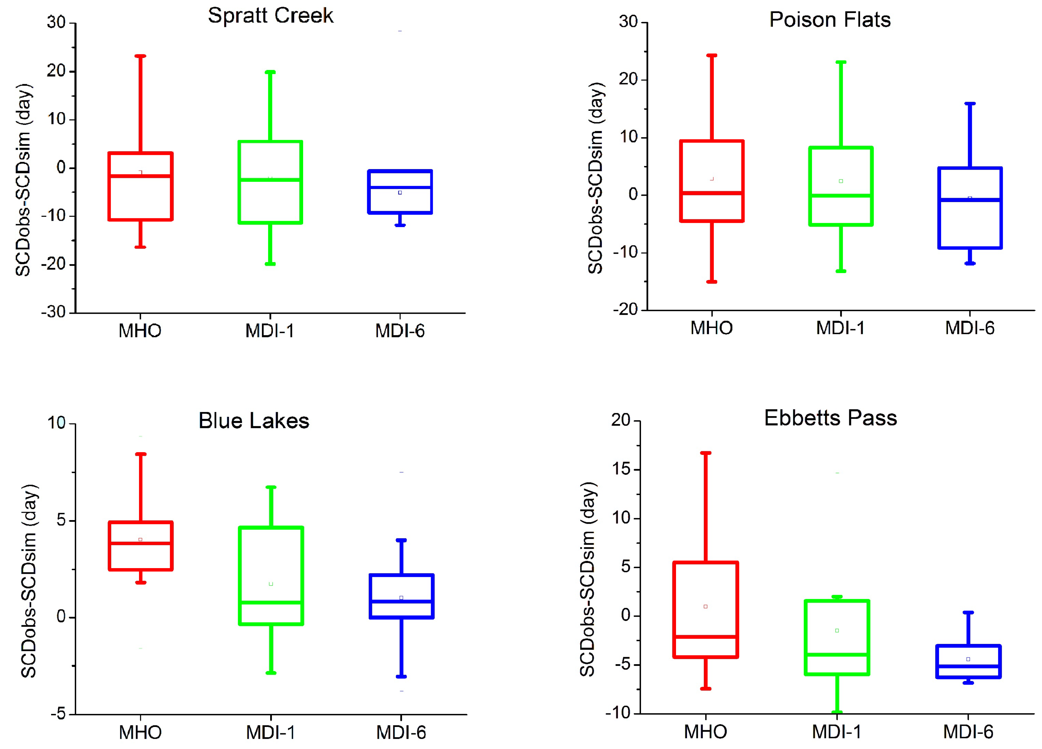
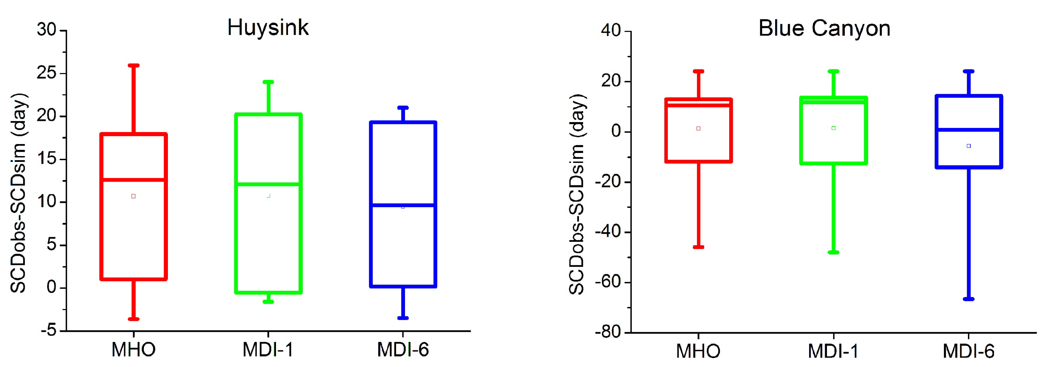
With regards to the data on the stations located at lower altitudes, the three snowmelt models overestimated the snow accumulation. The above results coincide with those registered by [57,58] who obtained better results in the SNOTEL stations located at a higher altitudes in the same basins with an increment of uncertainty for those stations at lower altitudes. The results of the MDI-1 and MDI-6 models are acceptable as those obtained in the DMIP2 Project by the SNOW-17 model (HL-RDHM and NWSRFS) and the TOPKAPI model that uses the energy balance [30]. In the calibration period, the best results in the modeling of snow point accumulation were obtained with the MDI-6 model. Therefore, the variability of the DDF positively influences and improves the approximation of the snow point accumulation. The results achieved in the validation period have again shown greater efficiencies in the Carson River basin in the SNOTEL stations located at a higher altitude. However, the biases show underestimations and overestimations of the three snowmelt models in both basins (Table 8). In the American River basin, the three snowmelt models do not adequately reproduce accumulation in the validation period. In general, an underestimation of snow accumulated at the monitor points is seen with respect to the observed data. On evaluating the models by SWE Centroid Data (SCD) it has been observed that the errors generalized in the two snowmelt models and for both basins is a product of the great heterogeneity of snow accumulation (Figure 7). Figure 7 shows that the MDI-6 model is the one that achieves a better approximation with lower SCD indices in the Carson River basin. In the American River basin, the three snowmelt models presented greater SCD indices with a greater uncertainty of the accumulation modeling in the two SNOTEL stations used (Figure 8).
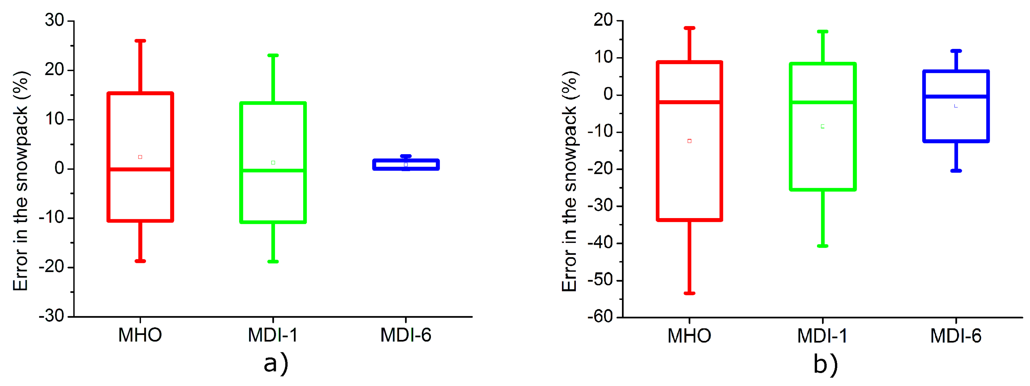
In the case of the spatial distribution of the snow, it was seen that the DDF variability has a very strong effect improving the results positively. That is, the modeled snowpacks have an excellent approximation to the snowpacks obtained from the satellite images when the DDF variability is used (Figure 9). The results also showed that the positive effect is greater when the six I R maps are used with the MDI-6 model (Figure 9). The former has demonstrated the importance of the energy flow from the SWR and the variables considered in its quantification such as topography, relief shading, and the zenith angle. In the same figure, we show that the MHO that uses homogeneous DDF obtained the worse results.
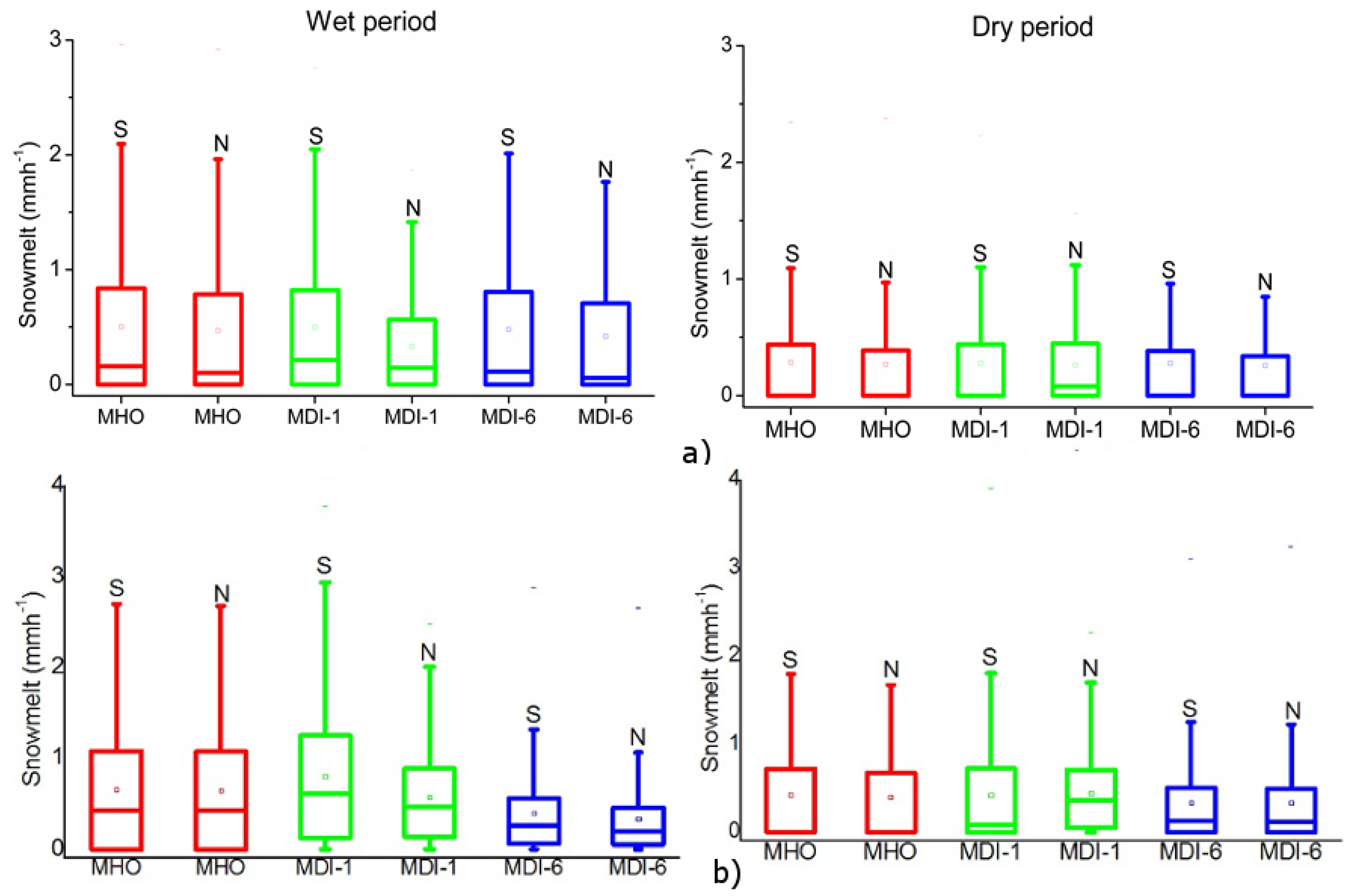
On analyzing the rates of snowmelt in the cells on the north and south hillside, important differences were also found in the snowmelt models. The greatest differences were recorded in the American River basin in the cells on the north hillside and for the wet period (Figure 10). The effect of the hillside is better represented by the MDI-6 model. The former is influenced by the number of I R maps used by this model. In the same figures, the MHO is not capable of differentiating the hillside using only the mean air temperatures and the homogeneous DDF. In quantitative terms, it has been estimated that the MHO melts some 19% more than the MDI-6 in the first months of winter in the cells on the north hillside of the Carson River basin. In the American River basin, it has been estimated that the MHO melts some 15% more than the MDI-6 in the first months of winter in the cells on the north hillside.
In the case of mass balance carried out in the selected cells, the results have shown the same behavior as the snowmelt rates in both basins. The MDI-6 model accumulates a greater amount of snow on the south and north hillside than the MDI-1 and MHO models. In the cells on the north hillside of the Carson River basin, an average accumulation of 64 mm more than that modeled with MHO has been estimated. In the American River basin, the MDI-6 accumulated an average of 63 mm more than the MHO in the north hillside cells.
In doing this research, the authors intended mainly that the greater advantage of the model MDI with respect to MHO was the way to simulate the spatial distribution of the snow, according to the observed SWE data and the snowpacks obtained from satellite images. In the first case (Figure 7 and Figure 8), it was interesting to note that the MDI-6 in higher-altitude basins better reproduces the punctual accumulation of the snow observed in the SNOTEL stations. With lower elevations in the American River basin, its snowmelt modeling becomes more complex even for energy balance models (references: [30,57]). In the case of the snowpack modeling, the MDI-6 surpass clearly the MHO (Figure 9), which is why we believe that this is the main advantage of the MDI-6 model with respect to the MHO and the true positive effect to include the spatio-temporal variability of the degree-day factor through the use of the I R maps.

7. Conclusions

In this research, the spatio-temporal variability of the degree-day factor in snow modeling using the degree-day method has been introduced using radiation index maps. The evaluation carried out has shown that the introduction of the spatial and temporal variability of these factors have positive effects on the hydrological modeling at catchment scale (i.e., at the outlet) and the simulation of the spatial and temporal variability of snow accumulation and snowmelt.
In the first case, the simulation of the discharges at the outlet of the two case studies is significantly improved when maps of radiation indices are used. In the calibration period and for both basins, the best degree-day snowmelt model has been the MDI-6, which uses six monthly maps of radiation indices. The MDI-6 model has also demonstrated a predictive ability superior to that of the MHO model with constant snow parameters, with very reasonable approximations in the temporal, spatial, and spatio-temporal validation. In fact, the results with MDI-6 are in the range of the best reported by [30] for these same basins in the DMIP2 project.
In many hydrological and environmental applications, a good spatial description of snow accumulation and melting is very important. In this sense, the results have shown that the spatio-temporal variability of the degree-day snowmelt factors significantly improve the simulation of snow accumulation when compared to the observations in the SNOTEL stations. In particular, the three distributed snowmelt models achieved good results in the stations located at a higher altitude and a greater uncertainty in those located at lower altitudes. This spatial pattern of the snow model reliability coincides with the results reported by [30,57]. Another very significant positive effect of the spatio-temporal variability of the snowmelt factors was observed in the spatial distribution of the snowpack. In this case, the MDI-6 model reached the best approximations to the snow cover observed by satellite images. These positive spatial results are highly relevant, since previous published research about improvements of the traditional MHO model, such as previous published research similar improvements of the traditional MHO model, such as [6,18,19,20,21], do not report this type of spatial validations.
Finally, it should be noted that the proposed distributed hydrological modeling with variable in space and time degree-day factor, does not imply a considerable additional effort compared with the modeling benefits: the needed radiation index maps can be easily computed from a DEM without increasing the information demand for the model implementation in high mountain basins.

Author Contributions

Conceptualization, I.O. and F.F.; investigation, I.O.; methodology, I.O. and F.F.; visualization, I.O.; calculation and formal analysis, I.O.; writing—original draft, I.O and F.F.; review and editing, J.M.

Funding

This study was supported by the Universidad de Guanajuato, Spanish National Parks Administration through the ACOPLA project (OAPN 011/2008), the Spanish Ministry of Science and Innovation through the projects ECO-TETIS (CGL2011-28776-C02-01), TETISMED (CGL2014-58127-C3-3-R) and TETISCHANGE (RTI2018-093717-B-I00).

Acknowledgments

The authors would like to thank the Engineering Division and the Directorate of Research and Postgraduate Support of the Guanajuato University, for the financial support granted to publish this article.

Conflicts of Interest

The authors declare no conflict of interest.

References

  1. Riboust, P.; Thirel, G.; Moine, N.L.; Ribstein, P. Revisiting a Simple Degree-Day Model for Integrating Satellite Data: Implementation of Swe-Sca Hystereses. J. Hydrol. Hydromech. 2019, 67, 70–81. [Google Scholar] [CrossRef]
  2. Beniston, M.; Farinotti, D.; Stoffel, M.; Andreassen, L.M.; Coppola, E.; Eckert, N.; Fantini, A.; Giacona, F.; Hauck, C.; Huss, M.; et al. The European mountain cryosphere: A review of its current state, trends, and future challenges. Cryosphere 2018, 12, 759–794. [Google Scholar] [CrossRef]
  3. Bernsteinová, J.; Bässler, C.; Zimmermann, L.; Langhammer, J.; Beudert, B. Changes in runoff in two neighbouring catchments in the Bohemian Forest related to climate and land cover changes. J. Hydrol. Hydromech. 2015, 63, 342–352. [Google Scholar] [CrossRef] [Green Version]
  4. Mateo-Lázaro, J.; Castillo-Mateo, J.; Sánchez-Navarro, J.I.; Fuertes-Rodríguez, V.; García-Gil, A.; Edo-Romero, V. Assessment of the Role of Snowmelt in a Flood Event in a Gauged Catchment. Water 2019, 11, 506. [Google Scholar] [CrossRef]
  5. Vormoor, K.; Lawrence, D.; Heistermann, M.; Bronstert, A. Climate change impacts on the seasonality and generation processes of floods & ndash; projections and uncertainties for catchments with mixed snowmelt/rainfall regimes. Hydrol. Earth Syst. Sci. 2015, 19, 913–931. [Google Scholar] [CrossRef]
  6. Kling, H.; Fürst, J.; Nachtnebel, H.P. Seasonal, spatially distributed modelling of accumulation and melting of snow for computing runoff in a long-term, large-basin water balance model. Hydrol. Process. 2006, 20, 2141–2156. [Google Scholar] [CrossRef]
  7. Verdhen, A.; Chahar, B.R.; Sharma, O.P. Springtime Snowmelt and Streamflow Predictions in the Himalayan Mountains. J. Hydrol. Eng. 2014, 19, 1452–1461. [Google Scholar] [CrossRef]
  8. Dudley, R.; Hodgkins, G.; McHale, M.; Kolian, M.; Renard, B. Trends in snowmelt-related streamflow timing in the conterminous United States. J. Hydrol. 2017, 547, 208–221. [Google Scholar] [CrossRef] [Green Version]
  9. Penna, D.; van Meerveld, H.; Zuecco, G.; Fontana, G.D.; Borga, M. Hydrological response of an Alpine catchment to rainfall and snowmelt events. J. Hydrol. 2016, 537, 382–397. [Google Scholar] [CrossRef]
  10. Vormoor, K.; Lawrence, D.; Schlichting, L.; Wilson, D.; Wong, W.K. Evidence for changes in the magnitude and frequency of observed rainfall vs. snowmelt driven floods in Norway. J. Hydrol. 2016, 538, 33–48. [Google Scholar] [CrossRef]
  11. Yilmaz, A.G.; Imteaz, M.A.; Ogwuda, O. Accuracy of HEC-HMS and LBRM Models in Simulating Snow Runoffs in Upper Euphrates Basin. J. Hydrol. Eng. 2012, 17, 342–347. [Google Scholar] [CrossRef]
  12. Costa, D.; Pomeroy, J.; Wheater, H. A numerical model for the simulation of snowpack solute dynamics to capture runoff ionic pulses during snowmelt: The PULSE model. Adv. Water Resour. 2018, 122, 37–48. [Google Scholar] [CrossRef]
  13. Meng, X.; Ji, X.; Liu, Z.; Xiao, J.; Chen, X.; Wang, F. Research on improvement and application of snowmelt module in SWAT. J. Nat. Resour. 2014, 29, 528–539. [Google Scholar]
  14. Fuka, D.R.; Easton, Z.M.; Brooks, E.S.; Boll, J.; Steenhuis, T.S.; Walter, M.T. A Simple Process-Based Snowmelt Routine to Model Spatially Distributed Snow Depth and Snowmelt in the SWAT Model1. JAWRA J. Am. Water Resour. Assoc. 2012, 48, 1151–1161. [Google Scholar] [CrossRef]
  15. Schilling, O.S.; Park, Y.J.; Therrien, R.; Nagare, R.M. Integrated Surface and Subsurface Hydrological Modeling with Snowmelt and Pore Water Freeze–Thaw. Groundwater 2019, 57, 63–74. [Google Scholar] [CrossRef] [PubMed]
  16. Semádeni-Davies, A.F. Representation of Snow in Urban Drainage Models. J. Hydrol. Eng. 2000, 5, 363–370. [Google Scholar] [CrossRef]
  17. Zaknic-Catovic, A.; Howard, K.W.; Catovic, Z. Modification of the degree-day formula for diurnal meltwater generation and refreezing. Theor. Appl. Climatol. 2017, 131, 1157–1171. [Google Scholar] [CrossRef]
  18. Hock, R. A distributed temperature-index ice- and snowmelt model including potential direct solar radiation. J. Glaciol. 1999, 45, 101–111. [Google Scholar] [CrossRef]
  19. Kustas, W.P.; Rango, A.; Uijlenhoet, R. A simple energy budget algorithm for the snowmelt runoff model. Water Resour. Res. 1994, 30, 1515–1527. [Google Scholar] [CrossRef]
  20. Braithwaite, R.J. Positive degree-day factors for ablation on the Greenland ice sheet studied by energy-balance modelling. J. Glaciol. 1995, 41, 153–160. [Google Scholar] [CrossRef] [Green Version]
  21. Cazorzi, F.; Fontana, G.D. Snowmelt modelling by combining air temperature and a distributed radiation index. J. Hydrol. 1996, 181, 169–187. [Google Scholar] [CrossRef]
  22. Hock, R. Temperature index melt modelling in mountain areas. J. Hydrol. 2003, 282, 104–115. [Google Scholar] [CrossRef]
  23. Francés, F.; Vélez, J.I.; Vélez, J.J. Split-parameter structure for the automatic calibration of distributed hydrological models. J. Hydrol. 2007, 332, 226–240. [Google Scholar] [CrossRef]
  24. Buendia, C.; Bussi, G.; Tuset, J.; Vericat, D.; Sabater, S.; Palau, A.; Batalla, R. Effects of afforestation on runoff and sediment load in an upland Mediterranean catchment. Sci. Total Environ. 2016, 540, 144–157. [Google Scholar] [CrossRef] [PubMed]
  25. Rogelis, M.; Werner, M.; Obregón, N.; Wright, N. Hydrological model assessment for flood early warning in a tropical high mountain basin. Hydrol. Earth Syst. Sci. Discuss. 2016. [Google Scholar] [CrossRef]
  26. Ruiz-Villanueva, V.; Stoffel, M.; Bussi, G.; Francés, F.; Bréthaut, C. Climate change impacts on discharges of the Rhone River in Lyon by the end of the twenty-first century: Model results and implications. Reg. Environ. Chang. 2015, 15, 505–515. [Google Scholar] [CrossRef]
  27. Orozco, I.; Ramírez, A.I.; Francés, F. Modelación de los impactos del Cambio Climático sobre los flujos y almacenamientos en una cuenca de alta montaña. Ing. Agua 2018, 22, 125–139. [Google Scholar] [CrossRef]
  28. McGrane, S.J.; Hutchins, M.G.; Miller, J.D.; Bussi, G.; Kjeldsen, T.R.; Loewenthal, M. During a winter of storms in a small UK catchment, hydrology and water quality responses follow a clear rural-urban gradient. J. Hydrol. 2017, 545, 463–477. [Google Scholar] [CrossRef] [Green Version]
  29. Li, Z.; Fang, H. Modeling the impact of climate change on watershed discharge and sediment yield in the black soil region, northeastern China. Geomorphology 2017, 293, 255–271. [Google Scholar] [CrossRef]
  30. Smith, M.; Koren, V.; Zhang, Z.; Moreda, F.; Cui, Z.; Cosgrove, B.; Mizukami, N.; Kitzmiller, D.; Ding, F.; Reed, S.; et al. The distributed model intercomparison project—Phase 2: Experiment design and summary results of the western basin experiments. J. Hydrol. 2013, 507, 300–329. [Google Scholar] [CrossRef]
  31. Simpson, J.J.; Dettinger, M.D.; Gehrke, F.; McIntire, T.J.; Hufford, G.L. Hydrologic Scales, Cloud Variability, Remote Sensing, and Models: Implications for Forecasting Snowmelt and Streamflow. Weather Forecast. 2004, 19, 251–276. [Google Scholar] [CrossRef] [Green Version]
  32. Jeton, A.E.; Dettinger, M.D.; Smith, J.L. Potential Effects of Climate Change on Streamflow, Eastern and Western Slopes of the Sierra Nevada, California and Nevada; US Department of the Interior, US Geological Survey: Washington, DC, USA, 1996.
  33. Rango, A.; Martinec, J. Revisiting the Degree-Day Method for Snowmelt Computations1. JAWRA J. Am. Water Resour. Assoc. 1995, 31, 657–669. [Google Scholar] [CrossRef]
  34. Garen, D.C.; Marks, D. Spatially distributed energy balance snowmelt modelling in a mountainous river basin: Estimation of meteorological inputs and verification of model results. J. Hydrol. 2005, 315, 126–153. [Google Scholar] [CrossRef]
  35. Kane, D.L.; Gieck, R.E.; Hinzman, L.D. Snowmelt Modeling at Small Alaskan Arctic Watershed. J. Hydrol. Eng. 1997, 2, 204–210. [Google Scholar] [CrossRef]
  36. Granberg, G.; Grip, H.; Löfvenius, M.O.; Sundh, I.; Svensson, B.H.; Nilsson, M. A simple model for simulation of water content, soil frost, and soil temperatures in boreal mixed mires. Water Resour. Res. 1999, 35, 3771–3782. [Google Scholar] [CrossRef]
  37. Viviroli, D.; Zappa, M.; Gurtz, J.; Weingartner, R. An introduction to the hydrological modelling system PREVAH and its pre- and post-processing-tools. Environ. Model. Softw. 2009, 24, 1209–1222. [Google Scholar] [CrossRef]
  38. Smith, T.J.; Marshall, L.A. Exploring uncertainty and model predictive performance concepts via a modular snowmelt-runoff modeling framework. Environ. Model. Softw. 2010, 25, 691–701. [Google Scholar] [CrossRef]
  39. Ohmura, A.; Kasser, P.; Funk, M. Climate at the Equilibrium Line of Glaciers. J. Glaciol. 1992, 38, 397–411. [Google Scholar] [CrossRef] [Green Version]
  40. Rich, P.M.; Dubayah, R.; Hetrick, W.A.; Saving, S.C. Using Viewshed models to calculate intercepted solar radiation: Applications in ecology. Am. Soc. Photogramm. Remote Sens. 1994, 1994, 524–529. [Google Scholar]
  41. Fu, P.; Rich, P.M. A geometric solar radiation model with applications in agriculture and forestry. Comput. Electron. Agric. 2002, 37, 25–35. [Google Scholar] [CrossRef]
  42. Duan, Q.; Sorooshian, S.; Gupta, V. Effective and efficient global optimization for conceptual rainfall-runoff models. Water Resour. Res. 1992, 28, 1015–1031. [Google Scholar] [CrossRef]
  43. Duan, Q.; Sorooshian, S.; Gupta, V.K. Optimal use of the SCE-UA global optimization method for calibrating watershed models. J. Hydrol. 1994, 158, 265–284. [Google Scholar] [CrossRef]
  44. Ajami, N.K.; Gupta, H.; Wagener, T.; Sorooshian, S. Calibration of a semi-distributed hydrologic model for streamflow estimation along a river system. J. Hydrol. 2004, 298, 112–135. [Google Scholar] [CrossRef] [Green Version]
  45. Perrin, C.; Michel, C.; Andréassian, V. Improvement of a parsimonious model for streamflow simulation. J. Hydrol. 2003, 279, 275–289. [Google Scholar] [CrossRef]
  46. Muttil, N.; Jayawardena, A.W. Shuffled Complex Evolution model calibrating algorithm: Enhancing its robustness and efficiency. Hydrol. Process. 2008, 22, 4628–4638. [Google Scholar] [CrossRef]
  47. Nash, J.; Sutcliffe, J. River flow forecasting through conceptual models part I—A discussion of principles. J. Hydrol. 1970, 10, 282–290. [Google Scholar] [CrossRef]
  48. Eckhardt, K.; Haverkamp, S.; Fohrer, N.; Frede, H.G. SWAT-G, a version of SWAT99.2 modified for application to low mountain range catchments. Phys. Chem. Earth Parts A/B/C 2002, 27, 641–644. [Google Scholar] [CrossRef]
  49. Kalin, L.; Govindaraju, R.S.; Hantush, M.M. Effect of geomorphologic resolution on modeling of runoff hydrograph and sedimentograph over small watersheds. J. Hydrol. 2003, 276, 89–111. [Google Scholar] [CrossRef]
  50. Merz, R.; Blöschl, G. Regionalisation of catchment model parameters. J. Hydrol. 2004, 287, 95–123. [Google Scholar] [CrossRef] [Green Version]
  51. Moriasi, D.; Arnold, J.; Van Liew, M.; Bingner, R.; Harmel, R.; Veith, T. Model evaluation guidelines for systematic quantification of accuracy in watershed simulations. Trans. ASABE 2007, 50, 885–900. [Google Scholar] [CrossRef]
  52. Kapnick, S.; Hall, A. Observed Climate–Snowpack Relationships in California and their Implications for the Future. J. Clim. 2010, 23, 3446–3456. [Google Scholar] [CrossRef]
  53. Singh, P.; Kumar, N.; Arora, M. Degree–day factors for snow and ice for Dokriani Glacier, Garhwal Himalayas. J. Hydrol. 2000, 235, 1–11. [Google Scholar] [CrossRef]
  54. Singh, V.; Singh, P.; Bishop, M.; Björnsson, H.; Haritashya, U.; Haeberli, W.; Oerlemans, J.; Shroder, J.; Tranter, M. Encyclopedia of Snow, Ice and Glaciers; Springer: Amsterdam, The Netherlands, 2011. [Google Scholar]
  55. Koren, V.; Reed, S.; Smith, M.; Zhang, Z.; Seo, D.J. Hydrology laboratory research modeling system (HL-RMS) of the US national weather service. J. Hydrol. 2004, 291, 297–318. [Google Scholar] [CrossRef] [Green Version]
  56. Ciarapica, L.; Todini, E. TOPKAPI: A model for the representation of the rainfall-runoff process at different scales. Hydrol. Process. 2002, 16, 207–229. [Google Scholar] [CrossRef]
  57. Shamir, E.; Georgakakos, K.P. Distributed snow accumulation and ablation modeling in the American River basin. Adv. Water Resour. 2006, 29, 558–570. [Google Scholar] [CrossRef]
  58. Shamir, E.; Georgakakos, K.P. Estimating snow depletion curves for American River basins using distributed snow modeling. J. Hydrol. 2007, 334, 162–173. [Google Scholar] [CrossRef]
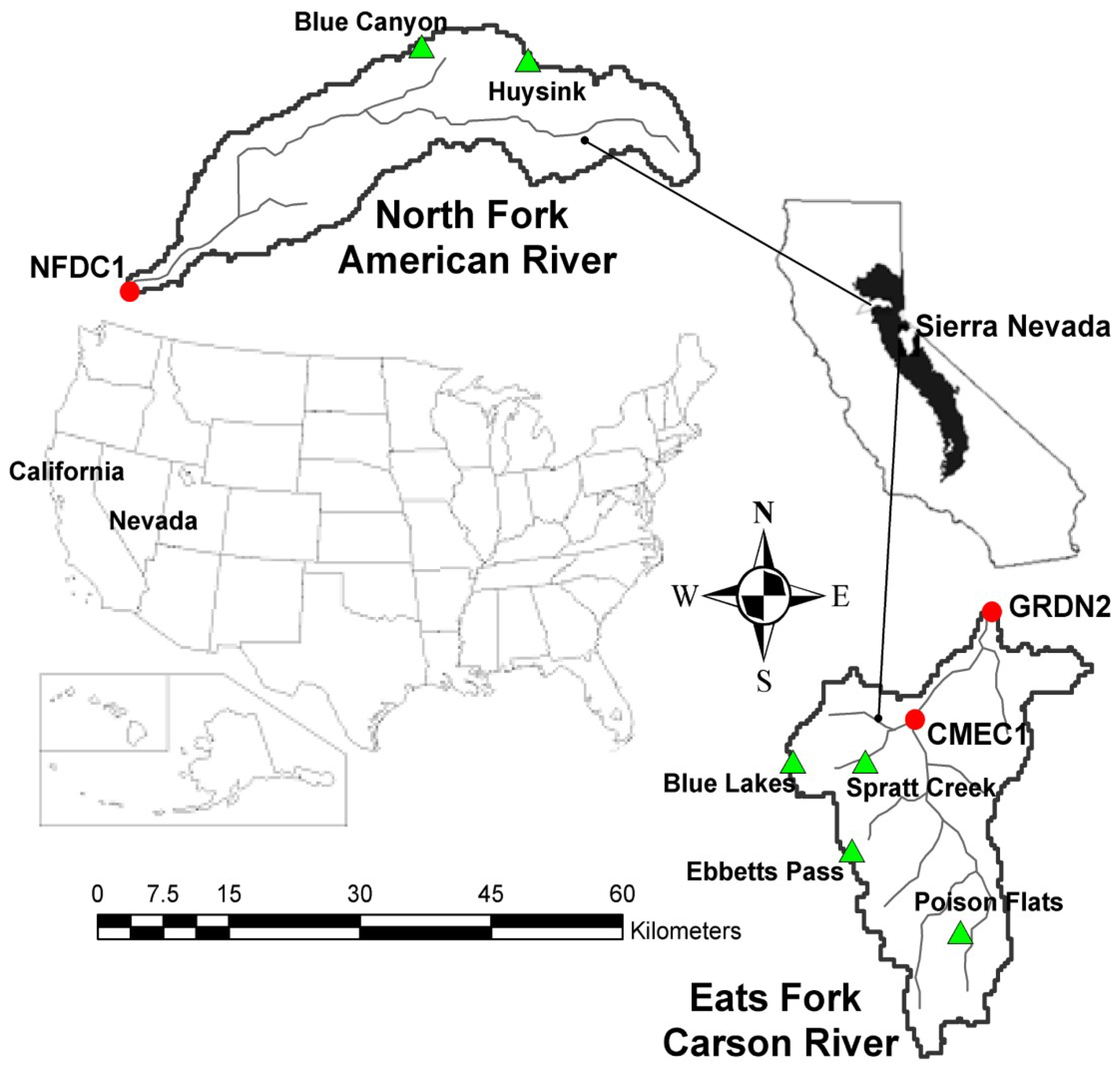
Figure 1. Location of the Carson and American basins in Sierra Nevada, USA, including the streamflow gauges () and SNOTEL stations ().
Water 11 01288 g001
Figure 2. Methodology implemented in the parsimonious modeling of high mountain basins.
Water 11 01288 g002
Figure 3. (a) Conceptual schema of tanks of the vertical movement at the level of the cell, (b) horizontal movement and connectivity of the TETIS model and (c) elements of the system, areas thresholds and components of the runoff.
Water 11 01288 g003
Figure 4. (a) Single map of radiation indices means and (bd) six maps of monthly indices of radiation used to introduce the variability of the degree-day factor (unitless).
Water 11 01288 g004
Figure 5. Spatial variability of the DDF1 achieved using the MDI-1 ( D D F 1 mean) and MDI-6 ( D D F 1 month) models in the (a) Carson and (b) American River basin.
Water 11 01288 g005
Figure 6. Modeling of observed flows in the control GRDN2 station in the Carson River basin (a) and NFDC1 station in the American River basin (b) for the period of calibration.
Water 11 01288 g006
Figure 7. SCD indices obtained by comparing the SWE observed and simulated within the period of calibration and validation to the Carson River basin.
Water 11 01288 g007
Figure 8. SCD indices obtained by comparing the SWE observed and simulated within the period of calibration and validation to the American River basin.
Water 11 01288 g008
Figure 9. Differences obtained in the distribution of snow when comparing satellite images and snowpacks obtained with the snowmelt models ((a) Carson River and (b) American River).
Water 11 01288 g009
Figure 10. Snowmelt rates modeled in south slope (S) and northern slope (N) in the year of the wet and dry period of calibration ((a) Carson and (b) American).
Water 11 01288 g010
Table 1. Runoff production parameters of TETIS model calibrated automatically with the SCE-UA algorithm.
ParameterCorrection FactorEffective Parameter
Static storage (mm) F C 1 H u ( i ) * = F C 1 · H u
Vegetation cover index ( ) F C 2 Λ * = F C 2 · λ v
Infiltration capacity (mmh 1 ) F C 3 k s ( i ) * = F C 3 · k s
Overland flow velocity (ms 1 ) F C 4 u ( i ) * = F C 4 · u
Percolation capacity (mmh 1 ) F C 5 k p ( i ) * = F C 5 · k p
Interflow velocity (mmh 1 ) F C 6 k s s ( i ) * = F C 6 · k s s
Deep aquifer permeability (mmh 1 ) F C 7 k p s ( i ) * = F C 7 · k s
Connected aquifer permeability (mmh 1 ) F C 8 k s a ( i ) * = F C 8 · k p s
River channel velocity (mms 1 ) F C 9 v ( t ) * = F C 9 · v ( t )
Table 2. Parameters of the snowmelt models calibrated automatically with the SCE-UA algorithm.
Snowmelt ModelParameterEffective Parameter
D D F 1 (mm C 1 d 1 ) D D F 1 * = D D F 1
MHO D D F 2 (mm C 1 d 1 ) D D F 2 * = D D F 2
T b ( C) T b * = T b
M f 1 (mm C 1 d 1 ) D D F 1 ( i ) * = M f 1 · I R ( i )
MDI M f 2 (mm C 1 d 1 ) D D F 2 ( i ) * = M f 2 · I R ( i )
T b ( C) T b * = T b
Table 3. Periods used in the warm up, calibration, and validation of the models in the Sierra Nevada basins.
Modeling PhaseGRDN2 (1)CMEC1 (1)NFDC1 (2)
Warm UpOct./1991–Sep./1992Oct./1991–Sep./1992Oct./1991–Sep./1992
CalibrationOct./1992–Sep./1994 Oct./1992–Sep./1994
Temporal validationOct./1994–Sep./2000 Oct./1994–Sep./2000
Spatial validation Oct./1992–Sep./1994
Spatio-temporal validation Oct./1994–Sep./2000
Gauges Carson basin ( 1 ) and American basin ( 2 )
Table 4. Average effective parameters of the TETIS model and effective parameters of the snowmelt models obtained in the Carson and American River basin.
Effective Carson Basin American Basin
ParameterMHOMDI-1MDI-6MHOMDI-1MDI-6
H u * 112.43125.6113.31192.33187.16200.07
Λ * 0.770.500.521.381.341.30
k s * 30.0243.5226.5118.6418.6417.70
u * 2.941.560.692.742.312.58
k p * 8.3919.4714.474.896.664.80
k s s * 16.1 × 10 3 21.6 × 10 3 12.3 × 10 3 5.8 × 10 3 6.3 × 10 3 6.9 × 10 3
k p s * 0.891.431.960.00.00.0
k s a * 41.70301.8858.0133.6585.3032.30
v * 1.360.871.290.991.321.04
D D F 1 * 3.391.2–3.70.34–3.903.510.93–4.80.23–3.21
D D F 2 * 3.171.3–4.00.7–7.37.961.19–6.20.24–3.40
T b * 2.541.802.912.051.641.17
Table 5. Statistical of efficiencies obtained by the models in the simulation of the streamflow for the period of calibration in the Carson and American basin.
GaugesStatistics Wet Period Dry Period
MHOMDI-1MDI-6MHOMDI-1MDI-6
GRDN2NSE0.9260.8770.9000.3510.4250.737
RMSE (m 3 s 1 )4.4925.8235.3164.7874.5083.049
NFDC1NSE0.8960.8940.890<0<00.573
RMSE (m 3 s 1 )11.99912.11712.3149.9428.1044.994
Table 6. Efficiencies obtained in the validations of the streamflow for the Carson and American basin.
BasinGaugesModelNSERMSE (m 3 s 1 )
MHO0.75629.975
AmericanNFDC1 (temporal)MDI-10.74334.814
MDI-60.78629.721
MHO0.7578.967
GRDN2 (temporal)MDI-10.7359.358
MDI-60.8107.930
MHO0.8734.437
CarsonCMEC1 (spatial)MDI-10.8754.399
MDI-60.8814.289
MHO0.66411.820
CMEC1 (spatio-temporal)MDI-10.68211.495
MDI-60.75110.186
Table 7. Efficiencies obtained by the DMIP2 models and TETIS-snowmelt models, in the period of temporary validation (Oct./1994–Sep./2000).
ModelsCarson Basin (GRND2)American Basin (NFDC1)
NSERMSE (m 3 s 1 )NSERMSE (m 3 s 1 )
HL-RDHM0.914.850.8917.92
NWSRFS0.885.680.8917.91
TOPKAPI0.817.010.8719.68
GR4J0.806.570.7328.89
TETIS-MHO0.777.700.7627.12
TETIS-MDI-10.758.040.7726.87
TETIS-MDI-60.856.750.8325.93
Table 8. Efficiencies obtained in the modeling of the accumulation of snow (SWE) in the SNOTEL stations in the calibration period for the Carson and American basin.
BasinSNOTELModel Calibration Validation
NSERMSE (mm)NSERMSE (mm)
Blue CanyonMHO0.65980.8990.28499.950
MDI-10.54793.2800.210104.96
American(elev. 1609 m)MDI-60.273118.1030.079113.313
HuysinkMHO0.789174.596<0559.10
MDI-10.847148.7630.427538.85
(elev. 2011 m)MDI-60.900126.255<0551.976
Spratt CreekMHO<0119.857<090.600
MDI-10.15492.1570.38257.604
(elev. 1863 m)MDI-6<0106.279<088.920
Poison FlatsMHO0.84090.4590.701115.889
MDI-10.82195.9480.691117.939
Carson(elev. 2357 m)MDI-60.86782.8580.82488.921
Blue LakesMHO0.778175.000.885151.293
MDI-10.844146.8940.917128.082
(elev. 2455 m)MDI-60.878129.9340.936112.880
Ebbetts PassMHO0.871137.3880.902165.09
MDI-10.916110.980.892173.307
(elev. 2671 m)MDI-60.95482.3060.922147.37