Monitoring Nonrevenue Water Performance in Intermittent Supply

Abstract

Water utilities should monitor their nonrevenue water (NRW) levels properly to manage water losses and sustain water services. However, monitoring NRW is problematic in an intermittent water supply regime. This is because more supplied water to users imposes higher volumes of NRW, and supplying significantly less water results in an unmet water demand but interestingly less NRW. This study investigates the influence of the amount of water supplied to a distribution system on the reported level of NRW. The volume and indicators of NRW all vary with variations in the system input volume (SIV). This is even more critical for monitoring NRW for systems shifting from intermittent to continuous supply. To enable meaningful monitoring, the NRW volume should be normalised. Addressing that, this research proposes two normalisation approaches: regression analysis and average supply time adjustment. Analysis of the NRW performance indicators showed that regression analysis enables the monitoring of NRW and tracking its progression in an individual system only, but not for a comparison with other systems. For comparing (or benchmarking) a water system to other systems with different supply patterns, the average supply time adjustment should be used. However, this approach presents significant uncertainties when the average supply time is less than eight hours per day.

1. Introduction

Supplying water to the residents of a city while minimising water losses in distribution systems is a challenge faced by water utilities worldwide. Nonrevenue water (NRW) is the difference between the amount of water added to a distribution system and the amount sold to the customers [1]. The estimated global volume of NRW is 126 billion cubic metres per year, costing approximately US $39 billion annually [2]. NRW either originates from leakages that occur at mains, storage reservoirs and customer connections, or commercial losses that occur due to customer meter under-registration, errors in data handling and billing or unauthorised use. The impact of NRW is substantial [3,4], as it accounts for considerable water wastage, affects the technical stability of the water supply, deteriorates the quality of water and water services, increases the operating costs and reduces revenues that should sustain and expand access to water. Assessing NRW involves quantifying water losses in a particular system without considering their actual locations [5,6].

Measuring the level of NRW indicates the levels of water leaking through deteriorated pipes and levels of commercial losses and is also considered as an indicator of the operational efficiency of the water system, water utility governance and the physical condition of the water supply system [7,8,9,10]. The level of leakage is likely the most important single indicator of the efficiency of water utilities perceived by regulators, the public and the media [11]. Utilities and projects are typically evaluated based on preset criteria, among which the NRW level is important [12,13].

To help water utilities sustain their services and manage their losses, NRW levels should be properly monitored. This is a crucial step for effective water loss management [14,15] and becomes more critical for utilities with variations in water productions, such as those that shift from an intermittent to a continuous supply pattern. When the amounts of water produced and distributed are higher, water typically remains in networks for a longer time, presenting challenges such as longer leakages and more potential for theft and other apparent losses (AL). Similarly, when less water is supplied, the NRW volume will be lower and NRW performance indicators (PIs) imply more efficient performance, but this may not be the case. Although this issue appears critical and intuitive, it has not been recognised in the literature [16,17,18,19,20,21,22,23,24,25]. The influence of varying amount of supplied water on the amount of NRW triggers the question of what should be monitored: the volume of NRW or the management status of NRW. For intermittent supply, the aim should be to improve the service, increase the water production and move towards a continuous supply. However, in this context, it is challenging to monitor the progress of NRW management and intervention, as all PIs vary according to variations of supplied water.

This study elucidates the relationship between NRW and system input volume (SIV), and analyses the potential methodologies for monitoring NRW and assessing its performance in an intermittent water supply regime when the properties of the supplied water vary. This analysis can help water utilities to properly monitor NRW levels and alleviate the political pressure that may be subjecting NRW management to failure in situations where certain measures are not at fault, such as systems with increasing levels of supplied water or supply times. It also reveals the reality of poor performance when the NRW level is lowered due to a decrease in the amount of water supplied to customers, rather than the implementation of effective reduction measures. The paper first analyses the influence of changing the SIV by varying the supply time when the network status and pressure are constant on the volume and PIs of NRW. Then, it discusses the normalisation of the NRW volume and PIs through “when-system-is-pressurised” (w.s.p.) adjustment and regression analysis, using the city of Sana’a, Yemen, as a case study. Monitoring NRW management using the suggested normalisation approach in this paper is the way forward to monitor NRW management in intermittent supply. The paper first provides an overview of the case study and then compares NRW PIs with and without normalisation, highlighting the appropriate methodology of NRW management monitoring.

2. Research Methodology

2.1. Overview of Sana’a Water Supply

Sana’a City is the capital of Yemen, a water-scarce country in the Middle East. The water situation in the Sana’a Basin is severe, as the water table drops by 6–8 m annually [26]. The public water service of Sana’a provides water to 45% of the city’s population, and the remainder receives water from the private sector, mainly via water tankers. The utility serves 94,723 customers, constituting approximately 1.32 million consumers, overall. The only source of water is a deep aquifer, from which water is extracted at 114 wells with depths ranging from 600 to 1000 m below ground. The water supply in Sana’a is a combined system, employing both pumped and gravity supply processes, and approximately 50% of the network is mainly pumped from the headworks. The supply network is geographically divided into six administrative zones, and each zone is subdivided into distribution areas, in which a total of 369 areas are interlinked and multifed. The supply pattern in Sana’a is intermittent and insufficient, as it does not fully meet the customers’ demands.

One customer received water once a week, with an average supply time of 4.4 h/day, prior to the current severe situation in Yemen that began in March 2015 [27]. The shortage of water necessitates a rationing program, and the implementation of an intermittent supply has caused network deterioration, accompanied by water quality deterioration and inadequate pressure in sections of the network.

Figure 1 (continuous line) presents the volume and apparent trend of NRW based on data from Sana’a water utility for 2005–2015. The average level of NRW in Sana’a for the 10 years was 7.1 million cubic metres (MCM) (35% of SIV), without considering inaccuracies in the records of the production meter. Since 2011, Yemen has faced great instability, with fuel and electricity shortages, that has further impacted the water services in Sana’a. This situation became critical in 2015, when a Saudi-led military campaign began in Yemen. Consequently, the fuel and energy sources for water production from wells have further declined, reducing the amount of water supplied to customers. Accordingly, the NRW level was reported to have decreased significantly to 2.8 MCM (22% of SIV) in 2015 (Figure 1).

2.2. Analysis of NRW and SIV Trends

The trends of SIV, billed consumption and NRW were analysed over 10 years. Monthly measurements of SIV and billed consumption were obtained from the Sana’a water utility and then converted to annual volumes.

The monthly and annual volumes of NRW were then calculated using Equation (1) [16,28]. The trends of the volumes of NRW, SIV and billed consumption were analysed monthly and yearly. As NRW reduction activities are a combination of top-down and bottom-up approaches, the analysis was conducted at system-wide and district metered area [29] scales to investigate the agreement between the results obtained at both scales.

$$\mathrm{NRW}=\mathrm{SIV}-\mathrm{BC}$$

(1)

where NRW (m³/year) is nonrevenue water, SIV (m³/year) is the system input volume and BC (m³/year) is the billed consumption.

2.3. NRW Component Assessment

The volumes of NRW components were calculated using Equations (2) and (3).

$$\mathrm{NRW}=\mathrm{AL}+\mathrm{RL}+\mathrm{UAC}$$

(2)

$$\mathrm{WL}=\mathrm{NRW}-\mathrm{UAC}=\mathrm{AL}+\mathrm{RL}$$

(3)

where AL (m³/year) is the apparent losses, RL (m³/year) is the real losses, UAC (m³/year) is the unbilled authorised consumption and WL is the volume of lost water. The volume of UAC was estimated by auditing and analysing the records of the Sana’a water utility. The volume of the AL was estimated using the Apparent Loss Estimation equation, as elaborated by AL-Washali, Sharma and Kennedy [27]. The volumes of real losses (RL) and water loss were then calculated using Equations (2) and (3). Accordingly, the International Water Association (IWA) standard water balance was established for the Sana’a water supply system for 2009. As the data of 2015 are incomplete, the same estimated proportions of NRW components in 2009 were used to calculate the NRW components for the year 2015, and the results were then compared.

The uncertainties of the NRW components were analysed using the error propagation theory [30]. The general error theory equation is shown in Equation (4). Uncertainty for the addition and subtraction of two measurements was calculated using Equation (5), while uncertainty for multiplication and division was calculated using Equation (6).

$$Ɗ\mathrm{U}=\sqrt{{\left(\delta \mathrm{U}/\delta \mathrm{A}\right)}^2 {\left(\Delta \mathrm{A}\right)}^2+{\left(\delta \mathrm{U}/\delta \mathrm{B}\right)}^2 {\left(\Delta \mathrm{B}\right)}^2+{\left(\delta \mathrm{U}/\delta \mathrm{C}\right)}^2 {\left(\Delta \mathrm{C}\right)}^2+\cdots }$$

(4)

$$\Delta \mathrm{U}=\sqrt{ {\left(\Delta \mathrm{A}\right)}^2+ {\left(\Delta \mathrm{B}\right)}^2}$$

(5)

$$\Delta \mathrm{U}=\mathrm{U}\sqrt{ {\left(\frac{\Delta \mathrm{A}}{\mathrm{A}}\right)}^2+ {\left(\frac{\Delta \mathrm{B}}{\mathrm{B}}\right)}^2}$$

(6)

where A, B and C are independent, measurable quantities that will be used to obtain a value of some calculated quantity U; and ∆A, ∆B and ∆C are the uncertainties of variable A, B and C, respectively. Other statistical parameters have been calculated for the NRW components.

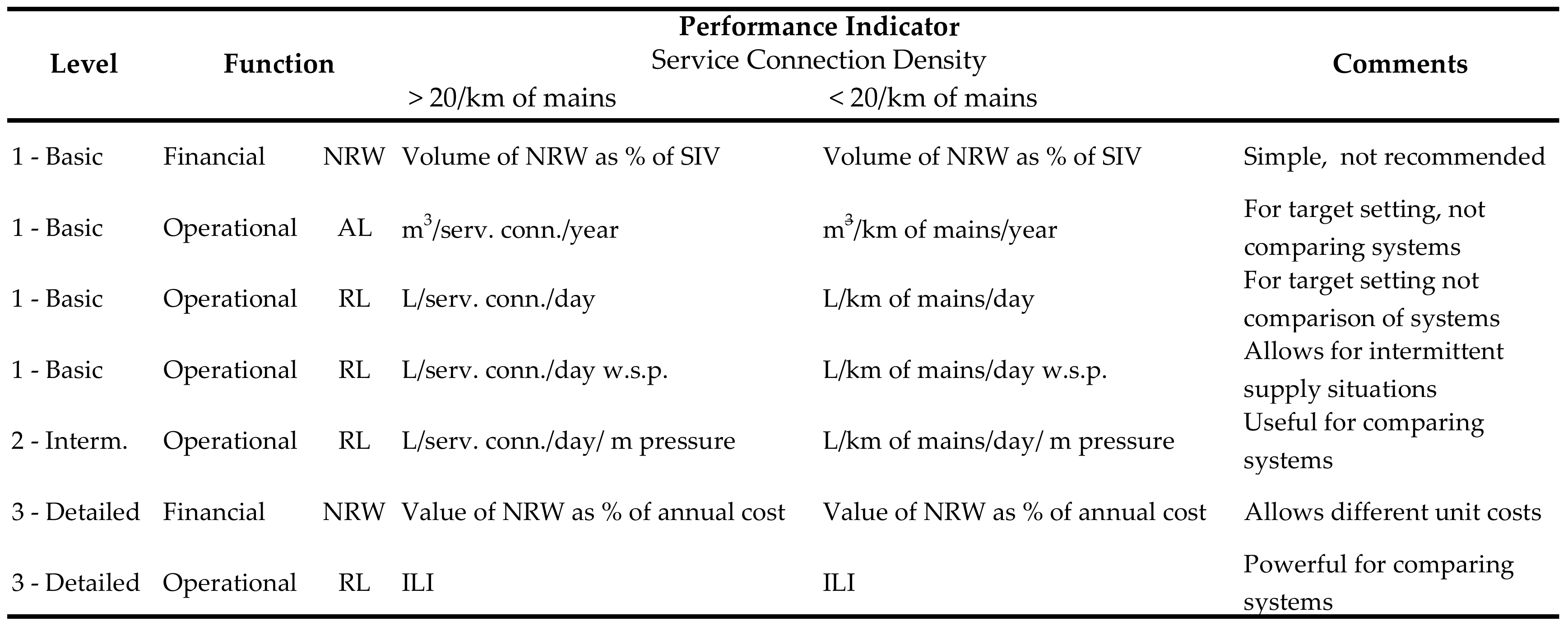
2.4. NRW Performance Indicators

Liemberger and Farley [31] and [16] recommended the IWA best practice PIs for NRW management, as presented in Figure 2. Frauendorfer and Liemberger [32] recommended the w.s.p. approach to normalise the overall level of NRW. In this approach, NRW is divided by the average supply time of the system, when the system is operated and water is supplied (h/day) and then multiplied by 24 (h/day). Because in an intermittent supply the average supply time is always less than 24 h/day, w.s.p. adjustment should in principle increase the NRW volume assuming the supply is continuous. For leakage monitoring and benchmarking, the European Commission [11] categorised two fit-for-purpose key performance indicators (KPIs) for targets and tracking progress in individual systems, including volume/year, m³/km of mains/day, litres/connection/day and litres/property/day. The KPIs for comparing internal/external leakage between different systems are the Unavoidable Annual Real Losses (UARL), Infrastructure Leakage Index (ILI), average pressure, value of leakage Euro/m³ and repair frequencies.

The infrastructure leakage index was calculated using Equation (7) [33].

$$\mathrm{ILI}=\frac{\mathrm{CARL}}{\mathrm{UARL}}$$

(7)

where ILI (unitless) CARL is the current annual RLs (m³/year) and UARL (m³/year) is the unavoidable annual RL, which can be calculated from Equation (8).

$$\mathrm{UARL} \left(\frac{\mathrm{Litres}}{\mathrm{serv}.\mathrm{conn}. \mathrm{day} }\right)=\left(18\times \frac{{\mathrm{L}}_{\mathrm{m}}}{{\mathrm{N}}_{\mathrm{c}}}+0.80+0.025{ \mathrm{L}}_{\mathrm{P}}\right)\times {\mathrm{P}}_{\mathrm{ave}}$$

(8)

where L_m is the length of mains in km, N_c is the number of service connections, L_p is the total length of private underground connection pipes in m (between the edge of the street and customer meters) and P_ave is the average operating pressure of the meters. Vermersch, Carteado, Rizzo, Johnson, Arregui and Lambert [28] suggested that the Apparent Loss Index could be used, which can be calculated in a similar manner to the infrastructure leakage index using Equation (9).

$$\mathrm{ALI}=\frac{\mathrm{CAAL}}{\mathrm{RAAL}}.$$

(9)

where ALI is the apparent loss index, CAAL (m³/year) is the current annual AL and RAAL (m³/year) is the reference annual AL, which represents 5% of the volume of the billed, authorised metered consumption, excluding exported water.

Suitable KPIs are essential for the effective monitoring and management of water loss. The package of NRW PIs should be designed as a “fit-for-purpose” set of indicators. However, they should be clearly defined, auditable, quantifiable, achievable and interpretable [11]. For Sana’a, the recommended, best-practice volume indicators of NRW and its components were calculated and adjusted to per-connection indicators as the service connection density in Sana’a is 97 service connections per km of mains. The per-pressure RL indicators and AL index were also calculated and analysed.

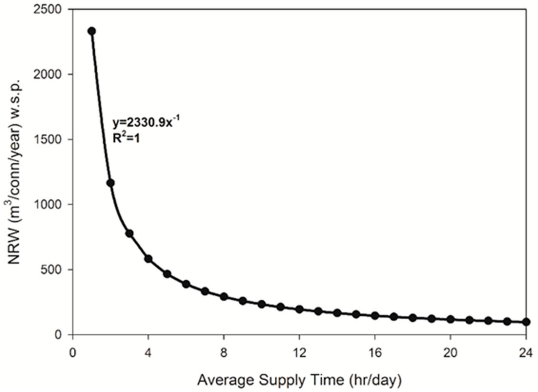
2.5. Normalising the NRW PIs Using w.s.p. Adjustment

‘When-system-is-pressurised’ adjustment is often used to normalise the PIs of the RL of systems with intermittent supply to allow comparison with other continuous supply systems. The volume of losses is adjusted as though the supply system is operating as a continuous supply. To generate ‘volume-per-day’ indicators following this approach, the annual volume of losses is not divided by 365 days, but by an equivalent number of pressurised days during the year. Alternatively, this can be achieved if the daily volume of losses is divided by the number of pressurised hours during the day and then multiplied by 24 h as shown in Equation (10) [32,34]. After this, the NRW PIs, particularly the infrastructure leakage index, can be compared to other systems with different supply patterns. Furthermore, the performance of the individual system should be monitored regularly when it has changing supply times.

$${\mathrm{NRW}}_{\mathrm{w}.\mathrm{s}.\mathrm{p}.}=\frac{\mathrm{NRW}}{{\mathrm{T}}_{\mathrm{avg}}}\times 24$$

(10)

where ${\mathrm{NRW}}_{\mathrm{w}.\mathrm{s}.\mathrm{p}.}$ (m³/year) is the normalised NRW and ${\mathrm{T}}_{\mathrm{avg}}$ is the average supply time in the system (h/day).

In this study, this approach is examined and extended to cover the volume of NRW, its components and PIs. The annual volumes of losses in Sana’a were transformed into daily losses by dividing the annual volumes of the NRW components by the equivalent number of days when the system was pressurised (operated), which was 69 and 9 days in 2009 and 2015, respectively. The NRW PIs were then calculated.

Sensitivity Analysis of the Average Supply Time (T_avg)

The sensitivity of the average supply hours during the day for the entire system, or, alternatively, the equivalent pressurised days during the year, was analysed to investigate its influence on the total volume of NRW and its PIs, and deepen our understanding of the impact and calculation of T_avg. The influence of T_avg on the volume of NRW was plotted on a curve, the equation was deduced and the step-slopes of the T_avg–NRW curve were analysed. Accordingly, the critical points of the curve and high-sensitivity cases were determined.

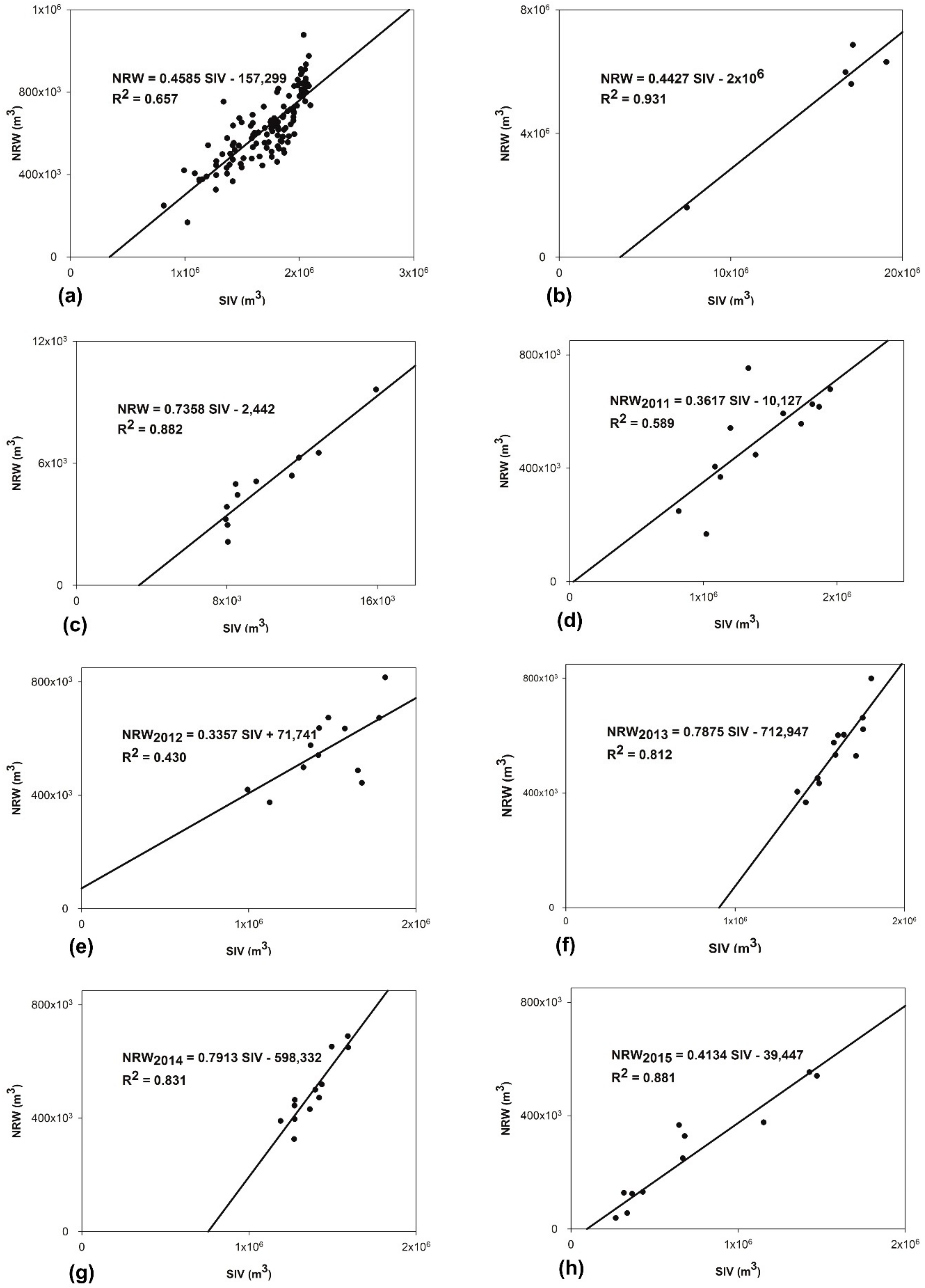
2.6. Normalising the NRW Using Regression Analysis

Another method for normalising the NRW volume and PIs is regression analysis using the NRW–SIV relationship when reliable historical data are available. In this approach, a reasonable correlation between NRW and SIV is first established, and the NRW volume and PIs can then be normalised and calculated for any production level of the given system or zone. This equation can be used as a baseline assessment of the status of NRW in the monitored system. When the NRW status must be evaluated again, another equation is generated, and the normalised volumes of NRW and PIs can be calculated for the same SIV to compare and assess any progression or regression in the NRW.

Extracting the Actual NRW Trend

The NRW–SIV regression equations were generated for 2011–2015 and the NRW levels were then normalised at a certain SIV, that is, the average of 2011–2015. The actual trend of NRW was plotted and analysed to track its progress in the Sana’a water supply system during this period and compare it to the unnormalised NRW trend.

3. Results and Discussion

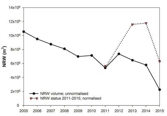
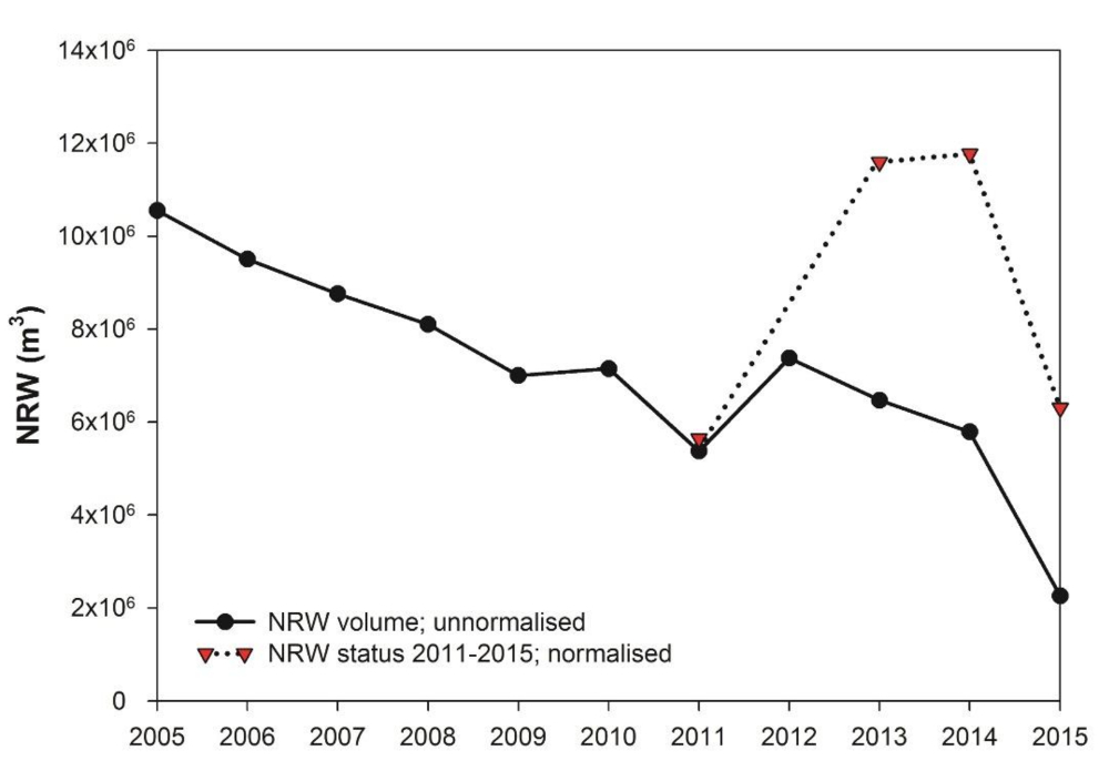
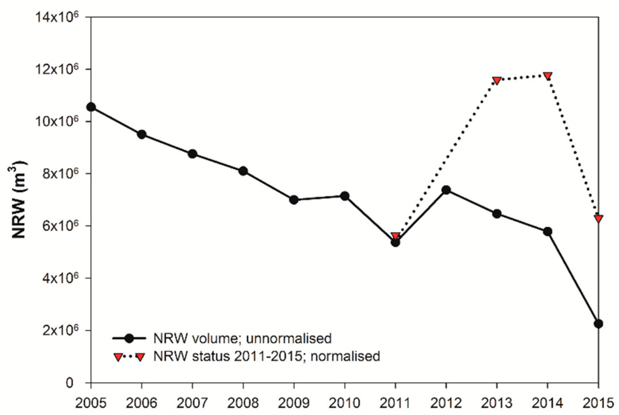
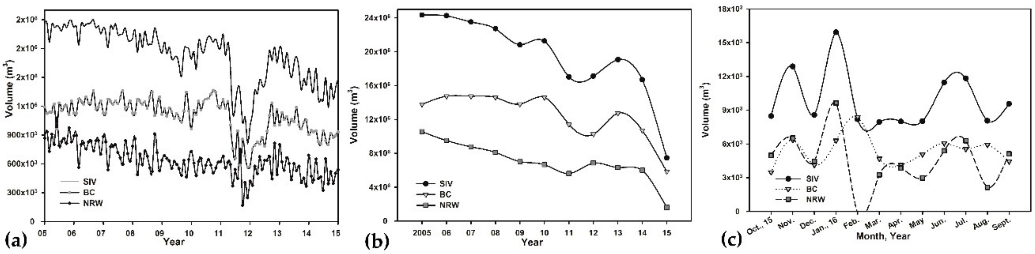
3.1. Fluctuations in the NRW Volume

Figure 3 shows the fluctuations in the NRW and SIV of the Sana’a water supply system under different production levels for the monthly and annual data. Figure 3a shows that the NRW increases and decreases following increases and decreases in the SIV. Figure 3b shows that the volume of NRW has decreased over time due to the decrease in the volume of SIV as a consequence of dwindling water resources in the Sana’a Basin. Figure 3c confirms the same behaviour using the monthly data of NRW and SIV for a small district metered area (DMA) within the Sana’a water network. There are anomalies at several points in Figure 3a,c, and some data are inaccurate for some months, especially for the DMA in Figure 3c at the beginning of the current conflict in Yemen, when the production and customer metering recording were unstable.

As shown in Figure 3, the volume of NRW varies with SIV, as it is higher or lower according to the SIV. This can also be concluded from the basic NRW equation. Consequently, the NRW volume and PIs all are affected by the volume of SIV. Therefore, it is more difficult to monitor the NRW level for intermittent supplies, as NRW PIs fluctuate according to the volume of supplied water.

This concern highlights the need for normalisation when reporting the NRW level for intermittent and fluctuating supplies.

3.2. NRW Components

The NRW components were estimated using the Apparent Loss Estimation equation elaborated by AL-Washali, Sharma and Kennedy [27].

Table 1. NRW components and uncertainties.

	Volume 2009	θ	SD	SD2	Volume 2015
	m3/year	± %	m3/year		m3/year
NRW	8,637,692	5	227,452	5 × 1010	1,604,557
UAC	114,152	20	11,648	1 × 1008	21,205
AL	5,686,452	18	531,632	8 × 1010	1,100,093
RL	2,837,088	40	578,363	1 × 1011	483,259

shows the volume of NRW components, 95% confidence limits (θ), standard deviation (SD) and variance (SD²) of NRW components. The proportions of NRW components were assumed to remain the same, and these proportions were used in the analysis of 2015, as shown in Table 1.

3.3. NRW PIs

Under the current conflict situation, the leaders of Yemeni water utilities compete over the limited available fuel in local markets to deliver as much water to customers as possible. The SIV has shrunk significantly from 22.3 MCM in 2009 to 7.4 MCM in 2015 due to electricity and power shortages. The length of the mains of the network and average pressure have remained the same, at 997 km and 10 m, respectively. In contrast, the number of water connections increased from 88,936 in 2009 to 94,723 in 2015.

Table 2. NRW PIs of Sana’a for 2009 and 2015.

NRW Component	PI	2009	2015	∆ %
NRW	m3/year	8,637,692	1,604,557	−81%
NRW	%	39%	22%	−44%
NRW	m3/c/year	97	17	−83%
RL	m3/year	2,837,088	527,024	−81%
RL	L/c/d	87	15	−83%
RL	L/c/d/m pressure	9	2	−83%
ILI	-	9	2	−82%
ILI	w.s.p.	48	62	+29%
AL	m3/year	5,686,452	1,056,328	−81%
AL	m3/c/year	64	11	−83%
ALI	-	8	4	−57%

compares the NRW volume and PIs for 2015 to those of 2009. All NRW PIs, expressed in different units, have reduced significantly, suggesting improved NRW performance. The PIs of the NRW components suggest the same. While all AL indicators suggest better performance, all RL indicators suggest the same, excluding the infrastructure leakage index when the intermittent supply was adjusted to be continuous (24/7) using the w.s.p. approach. This result suggests that volume-based indicators do not indicate the actual performance of the NRW status itself, but only their volumes, which vary according to changes in the SIV change. The actual NRW status performance can only be reflected in the NRW PIs when the w.s.p. adjustment is extended, to cover all NRW, AL and RL indicators.

3.4. Normalised NRW Using w.s.p. Adjustment

Table 3. Normalised NRW PIs of Sana’a for 2009 and 2015 using w.s.p. adjustment.

Component	PI	2009	2015	∆ %
Tavg	h/day	4.40	0.60	−86%
Tavg	day/year	66.92	9.13	−86%
SIV	m3/day w.s.p.	333,106	815,500	+145%
NRW	m3/day w.s.p.	129,081	175,842	+36%
NRW	m3/c/year w.s.p.	530	678	+28%
NRW	% w.s.p*	39%	22%	−44%
NRW	% w.s.p**	89%	98%	+10%
RL	L/c/d w.s.p.	477	610	+28%
RL	L/c/d/ m pres. w.s.p.	5	6	+28%
AL	m3/c/year w.s.p.	349	446	+28%
ILI	w.s.p.	48	62	+29%
ALI	w.s.p.	8	4	−57%
ALI	w.s.p.***	45	145	+219%

* adjusted SIV and BC for w.s.p.; ** adjusted SIV and unadjusted BC for w.s.p.; *** adjusted AL and unadjusted BC for w.s.p.

shows the normalised NRW PIs in Sana’a after normalising all figures to the w.s.p adjustment factor, as described in the methodology section. From Table 3, it can be concluded that the volumes and PIs of NRW and its components all increased significantly, indicating that the NRW status is worse, excluding the NRW as a percentage of SIV and AL index, which still indicate improvements in the NRW and AL.

For the NRW as a percentage of the SIV, the NRW % does not change from the figures in Table 2 if the SIV and billed consumption are adjusted to the same factor. However, if it is assumed that the billed consumption is not increasing, the water supply is sufficient and customers are saturated (which is not the case in Sana’a), the SIV will be adjusted and the NRW % of SIV will increase from 89% to 98% for 2009 and 2015, respectively. This further suggests worse performance, which is in line with the other PIs considered in this approach.

Similarly, for the AL index, when normalising the volumes of ALs and billed consumption to the same adjustment factor, the apparent loss index decreased from 9 to 4 in 2009 and 2015, respectively. However, if only the volume of the AL is adjusted and the billed consumption (BC) is not adjusted, the AL index also increased from 47 to 151 from 2009 to 2015, which corresponds with the other set of indicators.

Interestingly, there are great differences between the figures of the NRW PIs in Table 2 and Table 3. This suggests that the NRW PIs are sensitive to the adjustment factor used in this normalisation approach. Figure 4 shows the sensitivity of the NRW volume normalised through the w.s.p. approach to T_avg, which is used as an adjustment factor. It was found that when T_avg decreases, NRW increases. The power function of the curve is lim NRW = + ∞ when T_avg approaches zero from the right to the left. The derivatives of (T_avg) cannot determine the critical points of this curve. However, when benchmarking the volume of NRW at T_avg = 24 h/day and analysing the step-slopes of the curve from right to left, the results show that the volume of NRW will be doubled at T_avg = 12 h/day. Similarly, NRW will increase by 200%, 500% and 2300% when T_avg is 8, 4 and 1 h/day, respectively. The lower the T_avg, the more sensitive the normalised NRW volume. For the case of Sana’a, where T_avg was 4.4 and 0.6 h/day for 2009 and 2015, respectively, the normalised NRW volume becomes more sensitive. Thus, the accuracy of the analysis of all NRW components and PIs is significantly influenced by the calculation of T_avg.

However, calculating T_avg also has uncertainties for intermittent supply systems. In Sana’a, estimating the supply time for each distribution area within a network of 369 distribution areas is complicated, as the time of the distribution valves’ closures and pumping hours of the wells and headworks must be recorded. These data are not currently available, and there would be uncertainties in their collection. Therefore, estimating the supply time for each distribution area would require significant effort and commitment. Such uncertainties significantly undermine the accuracy of normalising the NRW levels and PIs through this approach.

Additionally, w.s.p. adjustment could be extended to include AL. However, while w.s.p. adjustment is suitable for RL PIs under the same pressure and infrastructure conditions, adjusting the AL PIs leads to overestimating apparent losses at the point once the demand is met, and any further supplied water contributes to higher RL while the ALs remain constant. Therefore, adjusting the AL through this approach is susceptible to overestimation.

Is the NRW Status Progressing or Regressing?

It is unclear whether the NRW situation in Sana’a has worsened, improved or remained the same from 2009 to 2015. The changes (∆) in the NRW PIs show that, during the period of 2009–2015, the NRW level decreased by 83% of its volume and the NRW percentage decreased by 44% of its value according to the traditional approach in Table 2. However, when it is normalised by w.s.p adjustment, the volume of NRW increased by 28% and the value of NRW % increased by 10% if the billed consumption remained unadjusted, as described in Table 3. Although this ‘suggested worse performance’ corresponding with the poor performance of the utility during the same period is due to the reduced water supply, it is still unclear whether this increase in NRW (w.s.p.) is accurate and the NRW management policies need to be revised. This could also be due to the effect of the reduced supply time on the normalised calculations of the NRW PIs. To confirm the status of NRW, the NRW volume was normalised using another approach, through regression analysis.

3.5. Normalised NRW Using Regression Analysis

The progress of the NRW status can be tracked using regression analysis for the NRW and SIV when a reasonable correlation exists. An NRW–SIV regression equation can be generated for the baseline year, and another equation should be generated for the following year, or any assessment year. The NRW volume and PIs can then be normalised at the current or a previous SIV, and the results can be compared to track the progress of the NRW’s status.

Figure 5 shows the NRW-SIV correlations and regression equations; there was a correlation between NRW and SIV in the long term, calculated based on monthly data obtained from Sana’a’s water supply system for 2005–2015 (Figure 5a). The correlation is reasonable (R² = 0.66), even with the poor data obtained for some years during the analysis period. The NRW-SIV correlations were also strong for annual data obtained for five years (2011–2015) for the full-scale system (Figure 5b), as well as for a DMA within the network (Figure 5c).

Using the NRW–SIV regression equation for 2015, as presented in Figure 5h, the volume of NRW was normalised to the same production level of 2009. The results show that the normalised volume of NRW₂₀₁₅ was 9.01 MCM, while that of NRW₂₀₀₉ was 8.64 MCM. This slight difference in the level of NRW is reasonable in Sana’a and more rational than what was suggested by w.s.p. adjustment. While unnormalised NRW has exhibited a reduction in the NRW level by 81%, normalisation of the NRW level by regression analysis suggested an increase in the NRW level of 4%, and the w.s.p. approach suggested an increase of 36%.

The NRW components and PIs in 2015 can also be normalised using regression analysis and compared to those of 2009. However, as the differences in the level of NRW using regression analysis are slight and the component assessment used the same proportions as those in 2009, the NRW PIs remained very close or almost the same as those of 2009, which are presented in Table 2.

Tracking and monitoring the NRW status, volume and PIs for an individual system are different from benchmarking and comparing the given system to other systems with different water production levels in the country or around the world. The above analysis indicates that, while regression analysis can normalise the NRW level for monitoring the NRW status of the individual system, the extended w.s.p. approach is still more useful for benchmarking and comparing different systems. However, w.s.p. adjustment suggested better performance for water supply systems with increasing T_avg. Developing a correction or “reduction” factor curve similar to that in Figure 4, but in the 4th quadrant, could be useful for conducting a more rational benchmarking of different systems with different T_avg.

Extracted NRW Status Trend

To track the behaviour of the NRW status in Sana’a over 2011–2015, NRW–SIV regression equations were generated for each year based on monthly data, as shown in Figure 5d–h. The equivalent normalised NRW volumes for these years were then calculated at their average SIV. As the correlation factor of 2012 was not strong (Figure 5e), the NRW–SIV regression equation of 2012 was not used. The behaviour of the NRW status over 2011, 2013, 2014 and 2015 is indicated by the dotted line in Figure 1. Accordingly, the status of NRW worsened between 2011 and 2013. This is valid for Sana’a water supply system, where the instability of the country, which began in 2011, has caused a high increase in unauthorised consumption, and sudden electricity shut-offs have caused operational problems in the network. During 2014, the situation was nearly the same, with a slight increase of the NRW due to a natural increase in leakage and limited electricity shut-offs, as the Sana’a water utility adapted to the situation. During 2015, the NRW status improved significantly, which is also valid as the Sana’a water utility valved off specific transmission pipes that the utility believed to have been illegally connected to irrigate farms along these pipes and near the well fields. In 2015, the utility also cooperated with local authorities at a district level to install isolation valves and reinstall customer water meters that had been removed in 2011. These interpretations explain well the NRW normalised curve in Figure 1.

4. Conclusions

Monitoring NRW and PIs in an intermittent water supply regime is significantly influenced by SIV. For that, a better approach is required to monitor NRW management. The influence of the varying SIV on the reported volume of NRW was investigated using monthly data of water production and billed consumption in Sana’a’s water supply system for ten years. The NRW PIs were compared with and without the normalisation approach. Accordingly, the study concludes the following for intermittent water supplies:

• The volume and PIs of NRW all vary in direct proportion to the SIV. This is critical for monitoring the level and PIs of NRW for water systems with fluctuating SIV and utilities that are shifting from intermittent to continuous supplies. An increase in the NRW level does not necessarily indicate worse performance, as it could be due to an increase in the amount of supplied water. Additionally, a decrease in the NRW level does not necessarily mean better performance, as it could be due to a decrease in the supplied water. Therefore, normalisation is necessary to properly monitor and benchmark NRW PIs for intermittent supplies.
• The ’when-system-is-pressurised’ adjustment, which is often used for normalising RL indicators, could be extended to normalise the volumes of NRW, AL, RL and their PIs. However, this principle leads to an overestimation of the AL, which are still difficult to monitor. This is because, when the demand is fully met, any increase in the system input volume contributes to RL, while the AL remain the same. Another limitation of this approach is the sensitivity of the average supply time (T_avg), as its uncertainties significantly undermine the accuracy of the normalised NRW PIs, including those of the RL. In addition, this approach is likely biased towards water systems with an increasing water supply and vice versa. For water systems with a T_avg of less than 8 h/day, the results of this approach become more uncertain. Finally, it is not certain whether this approach indicates the actual extent of NRW progression or regression.
• For monitoring the NRW status of an individual water supply system, the NRW volume and PIs can be normalised through regression analysis. This approach reflects the actual behaviour of the NRW status and provides more rational progression and regression extents. However, this approach can only be used for monitoring the NRW for individual systems, and not for a comparison of different systems.
• Comparing and benchmarking a water supply system to other systems with reasonable accuracy does not appear to be possible. More analysis is required to allow proper benchmarking using ’when-system-is-pressurised’ adjustment, particularly for extending it to AL benchmarking. Until then, for more rational benchmarking through this adjustment, a correction factor curve for T_avg should be developed to enhance the monitoring of the NRW progression and reflect the situation of NRW for a given system among other systems with different supply patterns.
• Once an NRW monitoring tool is available, NRW management should start by network partitioning into DMAs, pressure management, active leakage detection surveys, active customer meter replacement policy and the detection of unauthorised uses. Moving towards a smart network is effective in NRW management, using smart metering, smart data acquisition and on-time acting and control.

References

1. Lambert, A.O.; Hirner, W.H. Losses from Water Supply Systems: Standard Terminology and Recommended Performance Measures; IWA the Blue Pages, International Water Association: London, UK, 2000; pp. 1–13. [Google Scholar]
2. Liemberger, R.; Wyatt, A. Quantifying the global non-revenue water problem. Water Sci. Tech.: Water Supply 2018, 19, 831–837. [Google Scholar] [CrossRef]
3. Pillot, J.; Catel, L.; Renaud, E.; Augeard, B.; Roux, P. Up to what point is loss reduction environmentally friendly? The LCA of loss reduction scenarios in drinking water networks. Water Res. 2016, 104, 231–241. [Google Scholar] [CrossRef] [PubMed]
4. Erickson, J.J.; Smith, C.D.; Goodridge, A.; Nelson, K.L. Water quality effects of intermittent water supply in Arraiján, Panama. Water Res. 2017, 114, 338–350. [Google Scholar] [CrossRef] [PubMed]
5. Puust, R.; Kapelan, Z.; Savic, D.; Koppel, T. A review of methods for leakage management in pipe networks. Urban Water J. 2010, 7, 25–45. [Google Scholar] [CrossRef]
6. AL-Washali, T.M.; Sharma, S.K.; Kennedy, M.D.; AL-Nozaily, F.; Mansour, H. Modelling the Leakage Rate and Reduction Using Minimum Night Flow Analysis in an Intermittent Supply System. Water 2019, 11, 48. [Google Scholar] [CrossRef]
7. Park, H.J. A Study to Develop Strategies for Proactive Water-Loss Management. Ph.D. Thesis, Georgia Institute of Technology, Atlanta, GA, USA, June 2007. [Google Scholar]
8. Wallace, L.P. Water and Revenue Losses: Unaccounted-for Water; American Water Works Association: Denver, CO, USA, 1987. [Google Scholar]
9. Male, J.W.; Noss, R.R.; Moore, I.C. Identifying and Reducing Losses in Water Distribution Systems; Noyes Publications: New Jersey, NJ, USA, 1985. [Google Scholar]
10. McIntosh, A.C. Asian Water Supplies Reaching the Urban Poor; Asian Development Bank: Metro Manila, Philippines, 2003. [Google Scholar]
11. European Commission. EU Reference document Good Practices on Leakage Management WFD CIS WG PoM—Main Report; European Commission: Brussels, Belgium, 2015. [Google Scholar]
12. KFW. Water Loss Reduction Programme: Evaluation Report; German Bank for Development (Kreditanstalt für Wiederaufbau): Frankfurt, Germany, 2008. [Google Scholar]
13. Van den Berg, C.; Danilenko, A. The IBNET Water Supply and Sanitation Performance Blue Book; World Bank Publications: Washington, DC, USA, 2010. [Google Scholar]
14. AL-Washali, T.; Sharma, S.; Kennedy, M. Methods of Assessment of Water Losses in Water Supply Systems: A Review. Water Resour. Manag. 2016, 30, 4985–5001. [Google Scholar] [CrossRef]
15. Mutikanga, H. Water loss management: tools and methods for developing countries. Ph.D. Thesis, IHE-Delft, Institute for Water Education, Delft, The Netherlands, 2012. [Google Scholar]
16. Alegre, H.; Baptista, J.M.; Cabrera Jr, E.; Cubillo, F.; Duarte, P.; Hirner, W.; Merkel, W.; Parena, R. Performance Indicators for Water Supply Services; IWA publishing: London, UK, 2016. [Google Scholar]
17. Pybus, P.; Schoeman, G. Performance indicators in water and sanitation for developing areas. Water Sci. Tech. 2001, 44, 127–134. [Google Scholar] [CrossRef]
18. Al-Ansari, N.; Alibrahiem, N.; Alsaman, M.; Knutsson, S. Water Supply Network Losses in Jordan. J. Water Resour. Prot. 2014, 6, 83–96. [Google Scholar] [CrossRef] [Green Version]
19. Korkmaz, N.; Avci, M. Evaluation of water delivery and irrigation performances at field level: The case of the menemen left bank irrigation district in Turkey. Indian J. Sci. Tech. 2012, 5, 2079–2089. [Google Scholar]
20. Ermini, R.; Ataoui, R.; Qeraxhiu, L. Performance indicators for water supply management. Water Sci. Tech.: Water Supply 2015, 15, 718–726. [Google Scholar] [CrossRef]
21. Staben, N.; Hein, A.; Kluge, T. Measuring sustainability of water supply: Performance indicators and their application in a corporate responsibility report. Water Sci. Tech.: Water Supply 2010, 10, 824–830. [Google Scholar] [CrossRef]
22. Cunha Marques, R.; Monteiro, A. Application of performance indicators to control losses-results from the Portuguese water sector. Water Sci. Tech.: Water Supply 2003, 3, 127–133. [Google Scholar] [CrossRef]
23. Carpenter, T.; Lambert, A.; McKenzie, R. Applying the IWA approach to water loss performance indicators in Australia. Water Sci. Tech.: Water Supply 2003, 3, 153–161. [Google Scholar] [CrossRef]
24. Renaud, E.; Clauzier, M.; Sandraz, A.; Pillot, J.; Gilbert, D. Introducing pressure and number of connections into water loss indicators for French drinking water supply networks. Water Sci. Tech.: Water Supply 2014, 14, 1105–1111. [Google Scholar] [CrossRef] [Green Version]
25. Mutikanga, H.; Sharma, S.; Vairavamoorthy, K.; Cabrera, E. Using performance indicators as a water loss management tool in developing countries. J. Water Supply Res. T. 2010, 59, 471–481. [Google Scholar] [CrossRef]
26. JICA (Japan International Cooperation Agency). The Study for the Water Resources Management and Rural Water Supply Improvement in the Republic of Yemen, Water Resources Management Action Plan for Sana’a Basin; Final Report; Japan International Cooperation Agency: Tokyo, Japan, 2007. [Google Scholar]
27. AL-Washali, T.M.; Sharma, S.K.; Kennedy, M.D. Alternative Method for Nonrevenue Water Component Assessment. J. Water Res. Plan. Man. 2018, 144, 04018017. [Google Scholar] [CrossRef]
28. Vermersch, M.; Carteado, F.; Rizzo, A.; Johnson, E.; Arregui, F.; Lambert, A. Guidance Notes on Apparent Losses and Water Loss Reduction Planning; Malta College of Arts Science and Technology: Paola, Malta, 2016. [Google Scholar]
29. Farley, M.; Trow, S. Losses in Water Distribution Networks; IWA publishing: London, UK, 2003. [Google Scholar]
30. Taylor, J. An Introduction to Error Analysis: The Study of Uncertainties in Physical Measurements; University Science Books: New York, NY, USA, 1997. [Google Scholar]
31. Liemberger, R.; Farley, M. Developing a nonrevenue water reduction strategy Part 1: Investigating and assessing water losses. In Proceedings of the IWA Specialized Conference: The 4th IWA World Water Congress Marrakech, Marrakech, Morocco, 19–24 September 2004. [Google Scholar]
32. Frauendorfer, R.; Liemberger, R. The Issues and Challenges of Reducing Non-Revenue Water; Asian Development Bank: Mandaluyong, Philippines, 2010. [Google Scholar]
33. Lambert, A.; Charalambous, B.; Fantozzi, M.; Kovac, J.; Rizzo, A.; St John, S.G. 14 years’ experience of using IWA best practice water balance and water loss performance indicators in Europe. In Proceedings of the IWA Specialized Conference: Water Loss 2014, Vienna, Austria, 31 March–2 April 2014. [Google Scholar]
34. Charalambous, B.; Laspidou, C. Dealing with the Complex Interrelation of Intermittent Supply and Water Losses; International Water Association: London, UK, 2017. [Google Scholar]
Figure 1. NRW volume (unnormalised, apparent trend) and NRW status (normalised trend) in Sana’a.
Water 11 01220 g001
Figure 2. Recommended NRW PIs. (adapted from [16,31]).
Water 11 01220 g002
Figure 3. Fluctuation in the NRW volume according to changes in SIV: (a) monthly basis for the full-scale system; (b) annual basis for the full-scale system; (c) monthly basis for DMA-1 in Hadda Zone, Sana’a.
Water 11 01220 g003
Figure 4. Sensitivity of the normalised NRW volume (w.s.p.) to the average supply time in Sana’a water distribution system.
Water 11 01220 g004
Figure 5. NRW–SIV regression equations; (a) monthly volumes for 2005–2015; (b) annual volumes for 2011–2015; (c) monthly volumes for a DMA in Sana’a; and (d)–(h) monthly volumes for 2011, 2012, 2013, 2014 and 2015, respectively.
Water 11 01220 g005