Reassessing Water Allocation Strategies and Conjunctive Use to Reduce Water Scarcity and Scarcity Costs for Irrigated Agriculture in Southern Brazil

Abstract

The lack of adequate management programs alongside water resources overexploitation have led to undesirable effects such as water shortages and economic losses in several regions. Optimized water allocation strategies using groundwater and surface water resources could reduce water scarcity and scarcity costs by exploring the advantages and peculiarities of each source, thus reducing the effect of variability and uncertainties on water availability. The aim of this study is to assess economic water allocation and the potential of conjunctive use of surface water and groundwater operations using a hydro-economic model to evaluate scarcity and scarcity cost at an irrigated agricultural region in Southern Brazil. Results indicated the possibility to reduce but not entirely eliminate, water scarcity and scarcity cost based solely on the reallocation of water among users and crops, without generating water deficit to users downstream. Results also pointed to the elevated potential of groundwater use as a component to reduce scarcity and its costs, mainly through economic optimized strategies integrated with surface water.

1. Introduction

The lack of adequate management programs alongside water resources overexploitation have left several water systems throughout the world vulnerable to climate variability, which is often perceived during periods of severe water scarcity crisis. In this context, when increasing water supply through new reservoirs and water transfers, it is difficult to justify due to ever growing costs, water management instruments and governance should seek out opportunities to improve economic efficiency in water allocation itself, as well as water operations in the watershed.

In watersheds where surface water and groundwater are important components of the water systems, taking advantage of their distinct and complementary nature is fundamental for water resources management [1]. The best approach to conjunctively use both water supply sources is not one that involves choosing either one or the other but rather one that determines how best to use both resources in a concomitant way to solve water scarcity problems and to increase the efficiency of allocation [2]. Conjunctive use can thus be effectively applied to maximize water use benefits through integrated management, both augmenting supplies, increasing water productivity and efficiency and also avoiding aquifer overdraft. Several past studies have indicated that conjunctive use operations bring much needed increased flexibility to improve water systems’ performance and capacity to adapt to future changing conditions [3]. Other studies have demonstrated that ending groundwater overdraft, albeit costly, can have its economic impact greatly reduced through groundwater banking and the use of conjunctive-use infrastructure [4,5]. The behavior of the stream/aquifer system is a key component that can be explored when looking for improved operations, as hydrologic trade-offs. In some systems the depletion caused by groundwater pumping recharges the aquifer, which can be used to dampen annual variations in pumping; the farther the wells are positioned away from the stream, the closer the aquifer depletion gets to the total pumping averaged (annual rate) [6].

More recently a sequential GA approach was applied to model conjunctive use with multi-objectives, providing trade-off curves between system reliability and costs [7]. An overview of simulation-optimization modeling for conjunctive use of surface and groundwater for sustainable agriculture was also presented, and while it is pointed out that a combination of both simulation and optimization approaches is recommended for better system representation, the examples presented still lack more detailed representation of system economic benefits [8]. This latter limitation was addressed in an investigation of the economic values for conjunctive use and water banking in California and its significant benefits in expanding conveyance and storage facilities to improve operation flexibility and water transfers [9]. An integrated hydrologic-economic model combining distributed groundwater simulation and stream-aquifer interaction for better representation of conjunctive use was also developed in Reference [10]. The authors pointed out that system capacity expansion would allow a more diverse set of water management and operation strategies, leading to significant economic benefits.

Hydrologic-economic (or hydro-economic) models represent, at a regional hydrological scale, the technical, environmental and economic aspects of the water systems, through the inclusion of the economic concepts in models of water resources management. These models are used to study new strategies that promote efficiency and transparency in water use, through the application of management strategies and policies [11]. The hydro-economic models differ from other models in terms of carrying out an economic value assessment, that is, the economic demands of water are included, as well as the cost and benefit relationships, so that both physical and economic information are integrated into a system. This system is characterized by several items such as hydrological flows (water balance, groundwater recharge and discharge, return flows, etc.), relevant infrastructures (such as channels, reservoirs, tubular wells, etc.) and economic values (costs and benefits) of the demands [11]. In Reference [12], the value of the water to different users (urban, agricultural and industrial) is used in a hydro-economic model to estimate the marginal economic value of surface and groundwater at different locations in a water system, which is useful in the design of water pricing policies in regions under scarcity.

Water laws and policies worldwide have long acknowledged that water has economic value and different approaches have been sought to communicate this to users and to derive water policies to address scarcity: in South America, Chile has fostered tradable water rights [13] while in Brazil the National Water Resources Policy has among its fundaments that water, while a scarce resource, has economic value, and created water charges as economic water management instruments [14]. In Europe, the European Union (EU) actions have identified seven policies for addressing water scarcity and drought issues and “putting the right price tag on water” is the first among them [15]. In this context, finding a water price tag that communicates scarcity to users and is also able to evaluate the economic benefits of improved water and scarcity allocation are necessary steps towards improved water policies which recognize the economic value of water and create incentive to rational use.

In this context, despite hydro-economic modeling approaches, like those presented before, being well known, their application and results—especially combined with broader watershed operations including groundwater use—need further application. In Brazil, a hydro-economic model to evaluate short-run impacts on agricultural income from changes in precipitation and irrigation water supply was proposed in the Buriti Vermelho experimental Basin [16]. A decision support system to generate a hydro-economic model to identify the economic optimal allocation of water in the Sao Francisco river basin was also studied [17]. However, none of those studies included explicit groundwater operations and explored the potential for conjunctive use. This paper presents an application that combines both approaches (economic water allocation and the potential of conjunctive use operations within it) in a region located on the Brazilian South, more specifically in the Rio Grande do Sul state, which presents high agricultural water demands and have faced scarcity and conflict among users despite a well distributed rainfall pattern and relatively abundant water resources, when compared to other Brazilian regions [18]. In this region, users are left to bear the economic impacts of water scarcity with a very limited basis (if any) to discuss other arrangements, negotiation and instruments to mitigate it. In Reference [19] we calculated that the scarcity costs in this region may have amounted to 90 million USD in the last 15 years. The main contribution of this paper is to address economic water allocation and to provide an example application of how this allocation may improve a system’s economic performance and how conjunctive use operations can contribute to it. The paper does not advocate a direct implementation of the water allocation solutions presented here, given other performance indicators are necessary but rather its use to foster the negotiation process among users, where it can be useful to identify economic trade-offs and design economic water management instruments including water tariffs, water markets and environmental accounts.

2. Materials and Methods

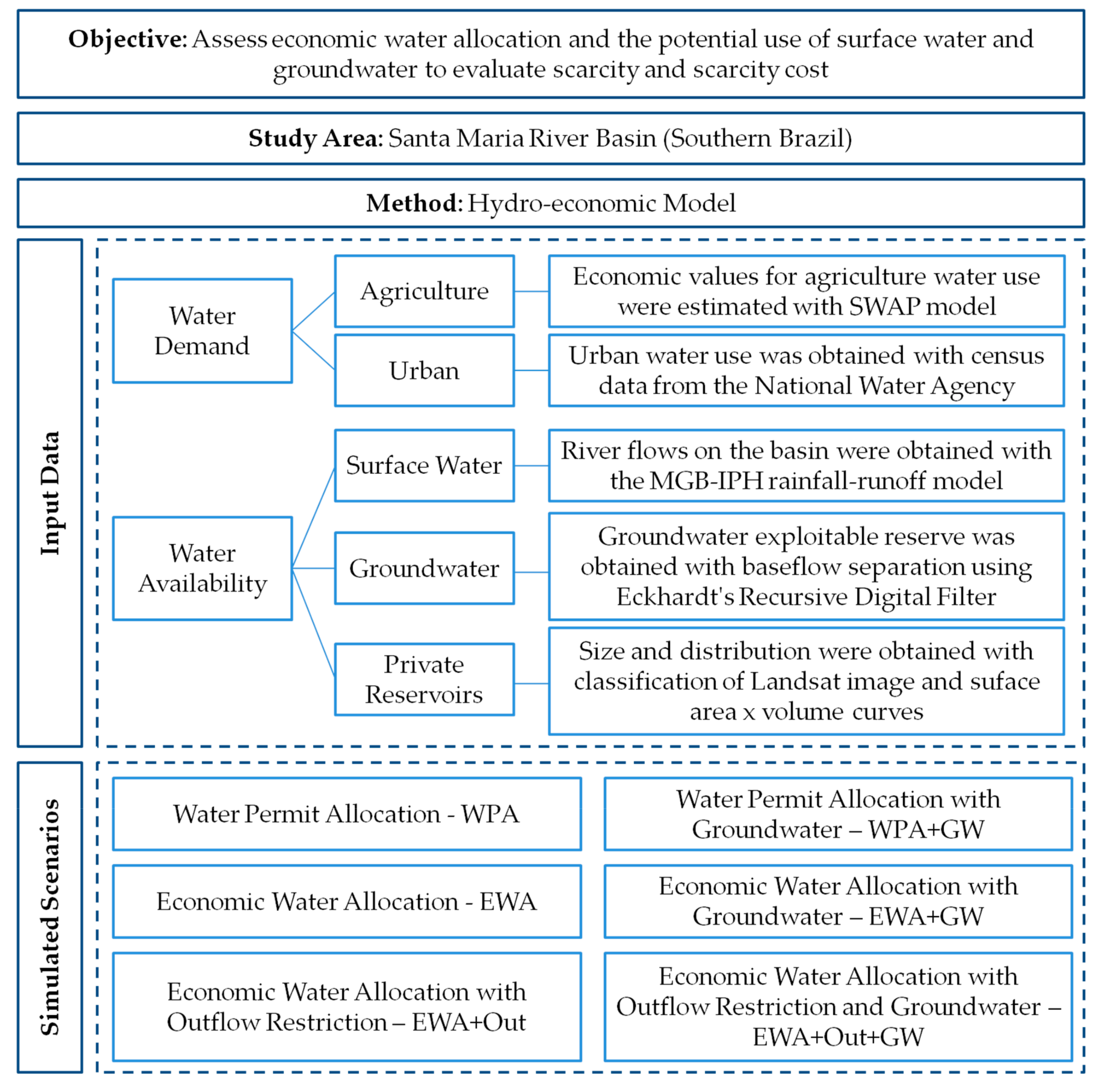
The modeling approach in this study uses a hydro-economic model to calculate water scarcity and scarcity costs, with and without conjunctive use strategies in the Santa Maria River basin system, located on the Rio Grande do Sul state in Southern Brazil. Economic agricultural production is obtained with the Statewide Agricultural Production Model (SWAP), which adopts positive mathematical programming for calibration [20]. The hydro-economic model solves the water allocation problem by following linear piece-wise economic penalty functions, developed from the marginal economic benefit functions calculated by SWAP, as in Reference [3]. Figure 1 displays a workflow that outlines the input data for the hydro-economic model and the simulated scenarios; in the next sections the methods are presented in further detail.

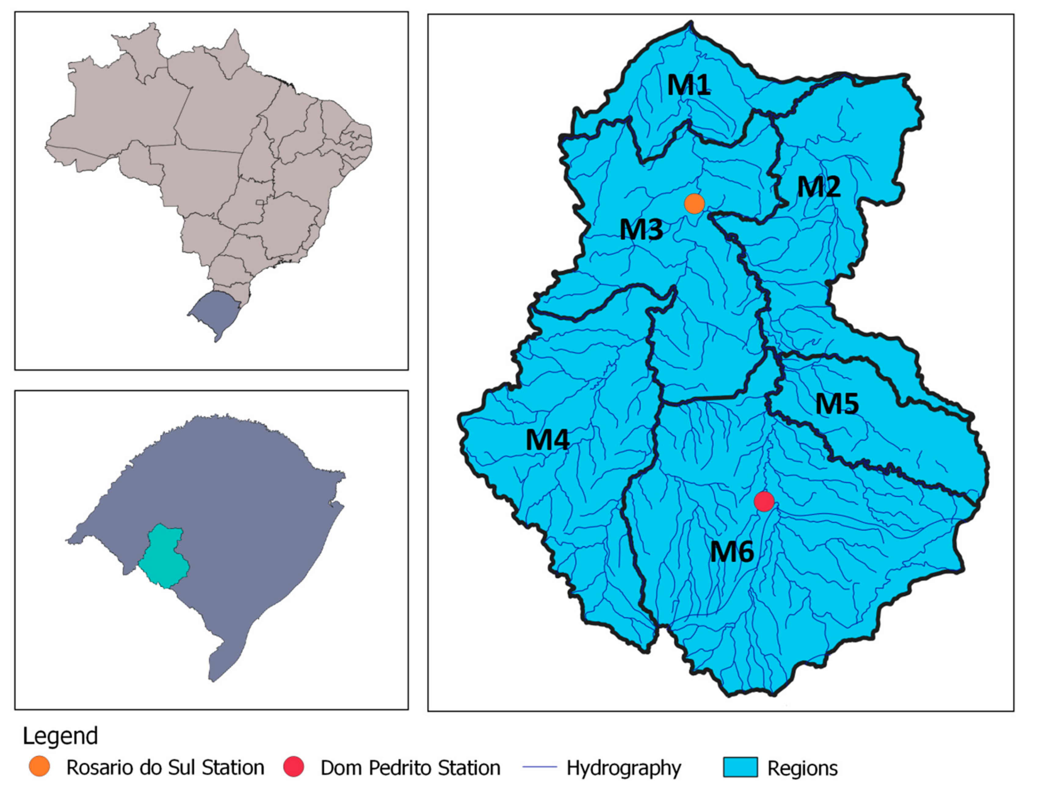
2.1. Study Site

The Santa Maria River Basin (SMRB) is located on the west region of Rio Grande do Sul state (Brazil), being part of the Hydrographic Region of the Uruguai River (Figure 2). SMRB comprises an area of approximately 15,790 km² [21]; 11% of its territory is used for soybean production and 6% for rice production, which are the two main crops on the basin [22]. Soybean is a temporary culture mostly irrigated with central-pivot systems and is cultivated in large continuous areas by gravity fed, flood irrigation [22]. The remaining land use in the region includes natural pasture that provides grazing for livestock.

A field visit to the study area was conducted to evaluate farmers’ perceptions of past losses and their association with water availability and water use decisions, as well as future expectations; the field visit was guided by members of the Santa Maria River Basin Water User Association (AUSM). Three farms that cultivated both soy and rice were visited; they were chosen because of their owners’ availability to show the area and describe their crop experience and mostly because the selected farms have representative agricultural and water use operations in the SMRB context. It was observed that the producers made several decisions based on water availability, such as defining the beginning of the growing season, the type of crop and the division of area between rice and soy. The visited farms have their own water reservoirs, some are filled exclusively through precipitation and local (within their property) flows (the volume depends on the contribution area of each reservoir and is also subject to variability in the rainfall regime). Other reservoirs are filled with rainfall complemented with water pumped from rivers nearby, to which the farmer withholds a water permit issued by the state water management agency. At the beginning of the cropping season, which may take place as early as October, the producer defines the amount of area to be planted with rice based on the amount of stored water in the reservoirs, in order to reduce the risk of production losses. Water needs include soil saturation, formation of a water table, plant evapotranspiration, deep percolation and compensation for lateral losses. Combined, those water needs amount to 8 to 10 thousand m³/ha. The irrigation period of BHSM rice crops occurs from October to February with the following distribution: 15% in October, 20% in November, 35% in December, 25% in January and 5% in February, which is the season of greatest water deficit, thus highlighting the importance of water storage in small farm-located reservoirs. This distribution is estimated based on the Santa Maria River Basin Water Plan [22] with modifications due to observed water demands and farmers’ reported experiences. It is important to note that the irrigation period can vary each year due to water availability and farmers’ decisions. Considering the whole SMRB watershed, the total area of rice crops is estimated at 110,039 ha and the annual demand to supply irrigation in this area is approximately 1100 hm³/year. Soy is a crop planted in alternation with rice, ensuring nitrogen fixation in the soil and offering an advantageous cost-benefit ratio for the farmer. The total area for soybean cultivation in the SMRB is 207,582 ha and the water demand is 830 hm³/harvest. Other less significant agricultural activities on the basin include maize, fruit and pasture.

The periods of significant drought in the Hydrographic Region of Uruguai River are associated with low rainfall occurrences. During these drought events, the intense use of water resources on the basin [23] aggravates drought impacts. Given the SMRB is a region subjected to water scarcity which relies mainly on surface water supplies but it has groundwater reserves available, it becomes an interesting study area for the investigation of the potential for implementation of conjunctive use and the exploration of economic water allocation and scarcity costs.

There are six municipalities on the SMRB. Given that economic and agricultural production is provided by census data on a municipality basis, those were used as water demand regions on SWAP and hydro-economic models. The regions can be seen on Figure 2 and the cropped areas of rice and soybean in each region are presented in

Table 1. Rice and Soybean Production.

Region		Rice (ha)	Soybean (ha)
M1	Cacequi	7656	7178
M2	Sao Gabriel	13,410	31,130
M3	Rosario do Sul	14,138	24,376
M4	Santana do Livramento	4053	15,225
M5	Lavras do Sul	1475	5710
M6	Dom Pedrito	42,985	71,563

. The SMRB was divided in homogeneous demand regions (M1 through M6). The distribution of observed cropping areas in each region appear in Table 1.

2.2. Economic Values for Agricultural Water Use

Agricultural economic values for water use were estimated for the six regions of the SMRB. For each region, an economic loss function was derived; these convex economic loss functions represent the reduction in net farm profits resulting from limited water delivery. The economic loss functions are based on the marginal benefit curves, which relate the marginal value of water to its availability. Thus, the scarcer the resource, the greater the benefit derived from its use [24,25]. The marginal benefit curves are used in hydro-economic models to simulate and model the users’ economic behavior, investigate different allocation policies and efficient water allocation decisions, amongst others [20,26].

On this study the marginal benefit curves were derived using SWAP (Statewide Agricultural Production Model), which is an optimization model that maximizes the sum of producer surplus (regional profits), that is, the economic benefit of farmers [20,27,28,29]. The model is defined over homogenous agricultural regions and it selects crops, water supplies and other inputs, subjected to constraints on water and land and economic conditions such as prices, yields and costs to optimize production and the economic benefit [20]. SWAP uses a Positive Mathematical Programming (PMP) approach to calibrate based on observed cropping areas [30]; the main advantages of PMP are auto calibration with exogenous variables (observed cropping areas) and the need for a small set of input data for a base year [28]. SWAP assumptions are that water is interchangeable across cultures and regions, that farmers try to maximize profit and that the selected crop mix is one that maximizes profits within a region.

The input data were obtained from several sources, including the Brazilian Institute of Geography and Statistics [21], the Brazilian Agricultural Research Corporation [31], Rio Grande do Sul Institute of Rice [32], Mato Grosso Institute of Agricultural Economy [33]. The data were also collected from a visit in the study area and with the members of Association of the Water Users of the Santa Maria River Basin. The SWAP calculation procedure is described in References [20,29]. GAMS (General Algebraic Modeling System) was used to solve the model [34]. A complete description of the SWAP methodology and results to the SMRB can be found at [19].

In order to generate the marginal benefit curves, the availability of water on SWAP was varied from 99% to 50% in successive model runs and after each run the Lagrange multiplier from the water availability constraint was recorded. The Lagrange multiplier indicates the water shadow value; according to the results, lambda values ranged from 0.02 R$/m³ (M1) to 0.31 R$/m³ (M4 and M5). At 99% availability of water, when the users have access to almost all water they need, lambda values ranged from 0.02 R$/m³ (M1) to 0.10 R$/m³ (M4 and M6). The marginal benefit curves are the result of a combination of several factors, such as water demand by culture, yield, selling price, costs of land, water and labor.

2.3. Urban Demand Data

The urban demands are responsible for the use of approximately 7.9 hm³/year of groundwater and 5 hm³/year of surface water [22]. There are four urban areas on the SMRB: Rosário do Sul and Dom Pedrito use water from rivers and reservoirs, Santana do Livramento and Cacequi use water from the aquifers. In the present study, the urban demands were based on urban census data [18] modeled with the highest priority.

2.4. Hydrological Data

Hydrological data in the hydro-economic model was used to represent local and incremental flows. In the present study these flows were obtained using the MGB-IPH model (Modelo de Grandes Bacias-Large Scale Basin Model) [35,36], which is a rainfall-runoff model semi-distributed and developed for the use on large basins (>10,000 km²). The hydrographic basin is separated in small unit-catchments and in each one is calculated a vertical balance of the soil water budget, which includes the evapotranspiration, precipitation, vegetation interception, soil infiltration and runoff generation, according to Equation (1). The generated volumes are transferred to linear reservoirs in each discrete basin and then are liberated through the drainage network; the discharges are propagated using the Muskingum-Cunge linear method. The GIS software MapWindow^® is used to run the MGB-IPH model [37] with the IPH-HydroTools [38].

$$\frac{\mathrm{dW}}{\mathrm{dt}}=\mathrm{P}-\mathrm{ET}-\mathrm{Dsup}-\mathrm{Dint}-\mathrm{Dbas}$$

(1)

where $\mathrm{W}$ (mm) is the water storage on the soil, $\mathrm{P}$ (mm/month) is the rainfall that reaches the soil, $\mathrm{ET}$ (mm/month) is the evapotranspiration from the soil, $\mathrm{Dsup}$ (mm/month) is the surface runoff, $\mathrm{Dint}$ (mm/month) is the subsurface flow and $\mathrm{Dbas}$ (mm/month) is the percolation to groundwater reservoir [36].

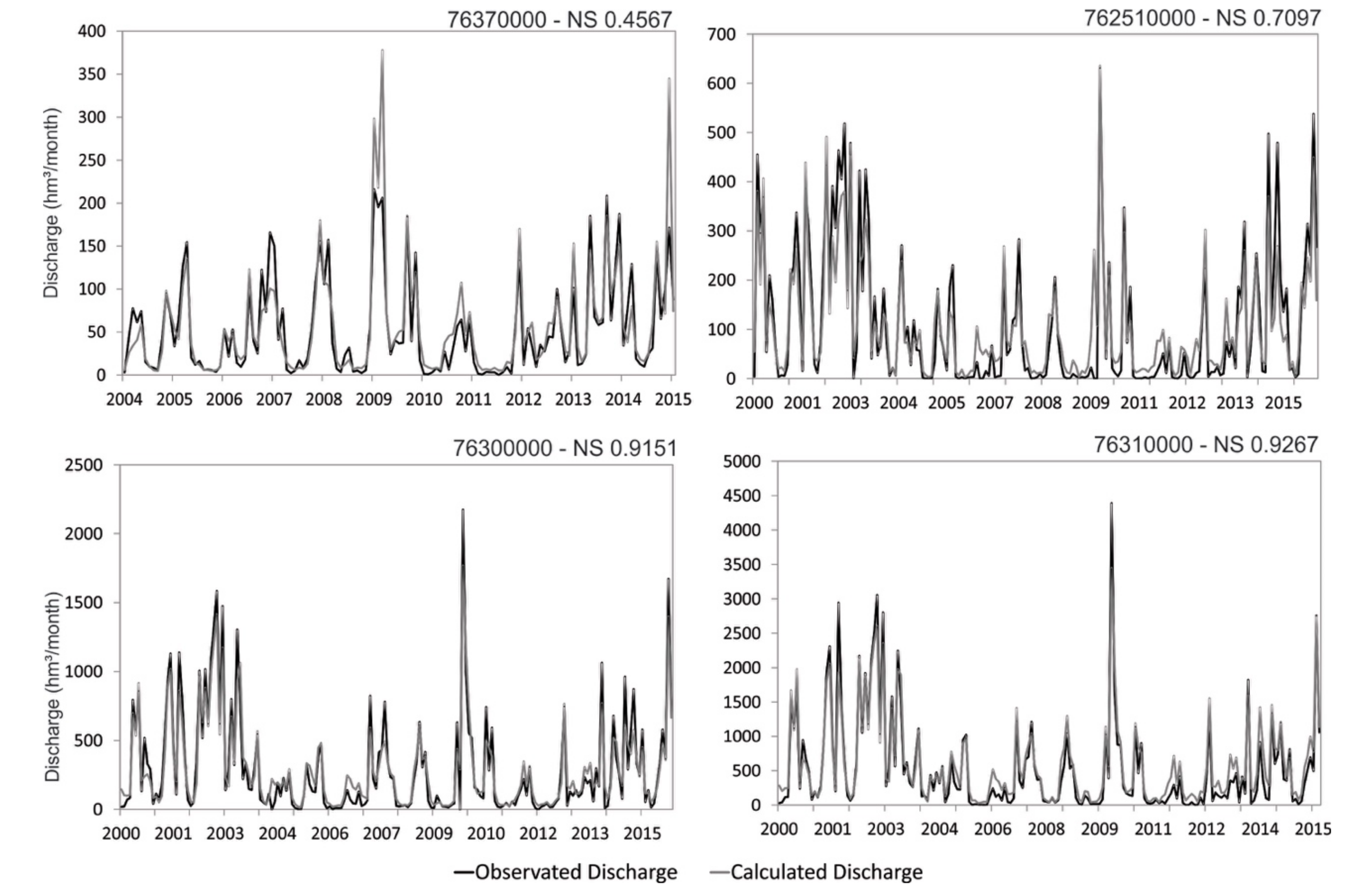
The MGB-IPH model used a digital elevation model from SRTM 90m as input data [39]; precipitation from the National Water Agency [40]; Hydrological Response Classes [41]; stream discharge from National Water Agency [40]. The hydrological simulation was executed from 2000 to 2015. The model was calibrated for four stations located on the SMRB (76251000, 76300000, 76310000 and 76370000); the calibration was intended to reproduce the discharge on the months that there were no water withdraws from the stream to irrigation, this way the model simulates the runoffs from the scarcity periods.

Figure 3 presents the calibration process for all stations and the Nash-Sutcliffe (NSE). On the station 76370000 the NSE of the simulation was 0.46; the difference between the simulated and the real discharge is mainly at higher values, this could be explained by the precipitation input, which can be overestimated by the model for this specific region. Also, this station has a shorter period of calibration than the other, from 2004 to 2015. The other stations had NSE that ranged from 0.71 to 0.93.

2.5. Groundwater Data

For conjunctive use, groundwater reserves must be investigated; here follows a description of the geological and hydrogeological framework of the SMRB area and the methods for the quantification of groundwater reserves.

Geological formations are very heterogeneous, ranging from sedimentary rocks such as sandstones and alluvial deposits, which have characteristics of aquifer formation, to fractured basaltic and crystalline rocks—such as the Serra Geral Formation—which has a good aquifer capacity and Crystalline Rocks, with a low potential aquifer. Regions predominantly composed of rocks belonging to the Guarani Aquifer System have a very important role in the relationship with surface water, since the vertical and effective infiltration processes are facilitated due to the great permeability of the surface layers. This description is based on the Geological Map of the State of Rio Grande do Sul, scale 1:750,000, prepared by the Brazilian Geological Survey [42]. Concerning the hydrogeology, the western portion of the basin presents high to medium capacity groundwater aquifers, while the eastern portion has medium to low capacity aquifers; this description is based on the Hydrogeological Map of the State of Rio Grande do Sul, scale 1:750,000, prepared by the Brazilian Geological Survey [43].

In this study, baseflow separation was made to estimate the aquifer recharge and to quantify the available reserves. This was done through the application of Eckhardt’s Recursive Digital Filter [44] with considerations proposed by Reference [45]. In this method baseflow in streams is calculated by separating the river flow into two components: direct flow (runoff) and indirect flow (baseflow) and then it is obtained the recharge rate, which is converted to the active reserve, according to Equations (2)–(4).

$${\mathrm{y}}_{\mathrm{i}}={\mathrm{f}}_{\mathrm{i}}+{\mathrm{b}}_{\mathrm{i}}$$

(2)

$${\mathrm{b}}_{\mathrm{i}}=\frac{\left(1-{\mathrm{BFI}}_{\max }\right)\times \mathrm{a}\times {\mathrm{b}}_{\mathrm{i}-1}+\left(1-\mathrm{a}\right)\times {\mathrm{BFI}}_{\max }\times {\mathrm{y}}_{\mathrm{i}}}{1-\mathrm{a}\times {\mathrm{BFI}}_{\max }}$$

(3)

$$\mathrm{RR}= \frac{ \overline{\mathrm{b}} }{\mathrm{A}}\times 1000\times 31622400$$

(4)

where $\mathrm{y}$ is the discharge; $\mathrm{f}$ direct flow (runoff); $\mathrm{b}$ is the baseflow; i is the time step; a is the recession constant; ${\mathrm{BFI}}_{\max }$ is the maximum Baseflow Index; $\mathrm{RR}$ is the aquifer recharge rate and $\mathrm{A}$ is the watershed area. More details about the method application on SMRB can be found in References [46,47].

Groundwater storage reserves can be classified into permanent reserves, which is the volume of water accumulated in the aquifer environment and does not respond to seasonal fluctuation of the potentiometric surface; and renewable reserves, which are the volumes stored between the levels of maximum and minimum fluctuation of aquifers, with annual variations due to the seasonal contributions of surface water and groundwater; the renewable reserves are related to the annual aquifer recharge [48,49]. The active groundwater reserve is defined as part of the renewable reserve (baseflow subtracted of the minimum river flow); and the exploitable reserve is defined as 50% of the active reserve. This is consistent with what was proposed by Reference [18], which allows for the sustainable use of groundwater resources. After baseflow separation, the groundwater active reserve was found to be 1432 hm³/year and thus, the exploitable reserve is 716 hm³/year for the whole SMRB. The maximum monthly groundwater withdrawals were defined by the baseflow average cycle.

2.6. Reservoirs Data

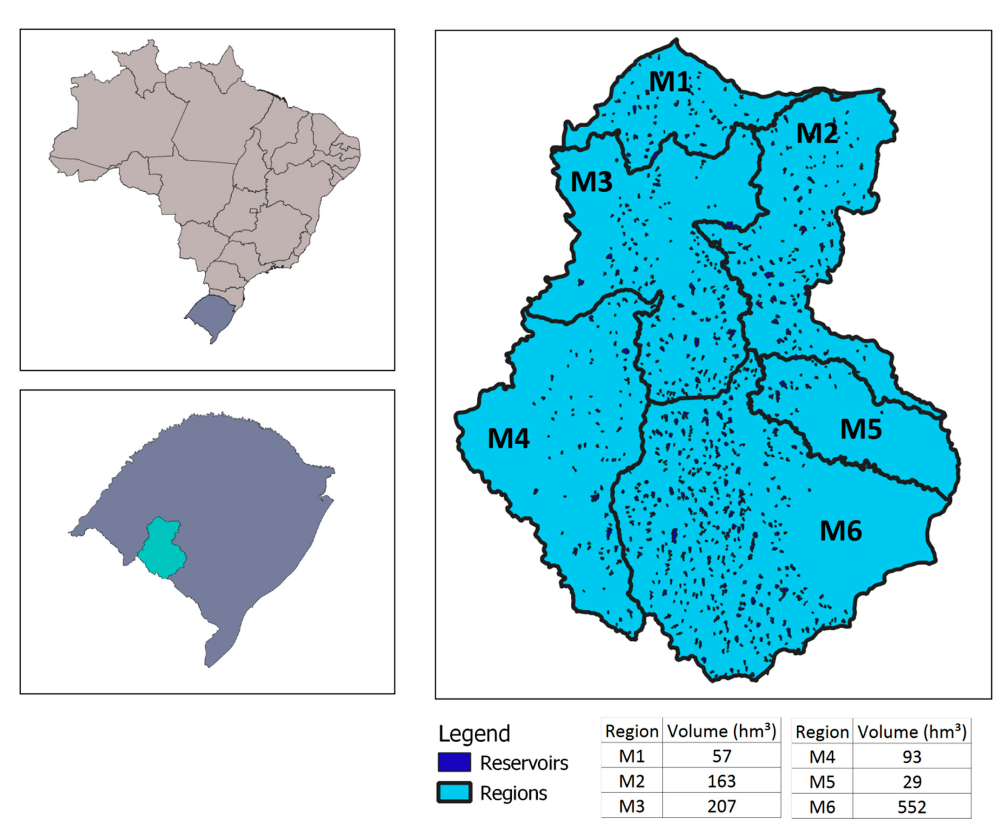
Farmers in the Santa Maria River Basin use private reservoirs to store water: most properties have their own reservoirs that are filled with water from the rain and with river withdraws, for which a permit from the state’s environmental office is necessary. Representing the reservoir dynamics is complicated because the farmer’s decision to use or store water depends on several factors and also because these private reservoirs are spread across the Basin area. In this study, the distribution and volumes of the private reservoirs was first obtained and then they were aggregated by region, which means we added the volumes of all reservoirs within each region. Thus, the hydro-economic model interprets this input as six reservoirs that correspond to the six regions of the SMRB presented before.

In order to define the distribution of the reservoirs, a classification of a Landsat image from the month of October of 2015 was made; this month was chosen because it is just before the beginning of the irrigation period and the reservoirs should be at their highest levels. The classification resulted in a total of 4195 reservoirs, corresponding to a wet area of 1101 hm³; Figure 4 indicates the distribution and volume of the reservoirs which have area over 10 ha. The relationship between surface area and volume was obtained through a curve available in Reference [22]; the combined storage capacity of the private reservoirs is an input for the hydro-economic model. It can be seen that regions M6, M3 and M2 have the higher amount of reservoirs.

2.7. Hydro-Economic Model

In order to perform water allocation among the economic demands, an optimization model was used [50]. The model builds a representation of the SMRB water demands, natural conveyance system (rivers), artificial conveyance (withdrawal and pumping infrastructure) artificial and natural water storage (reservoirs and aquifers). Water demands and storage are represented as nodes, while conveyance elements are represented as arcs, connecting different nodes. The model minimizes the total water scarcity cost, having as decision variables the amount of water withdrawn from each water storage node. The objective function has a list of penalty functions, one for each demand node and for each month, to calculate the total cost of water scarcity. Model constraints include mass balance at each node and physical constraints. GAMS (General Algebraic Modeling System [34]) was used to solve the model.

2.7.1. Input Variables and Equations

Mass balance (Equation (5)) calculates the storage on each node and time step. The variable ${\mathrm{LINK}}_{\mathrm{T},\mathrm{I},\mathrm{PT}}$ is the flow volume at time step T between nodes I and PT. $\mathrm{PER}$ is the infiltration on the river at each month, ${\mathsf{\alpha }}_{\mathrm{T},\mathrm{PT}}$ and ${\mathsf{\beta }}_{\mathrm{T},\mathrm{PT}}$ are evaporation parameters, ${\mathrm{S}}_{\mathrm{T},\mathrm{PT}}$ is the storage at node PT and time T. ${\mathrm{Q}}_{\mathrm{T},\mathrm{PT}}$ is the water influx at time T to node PT. The latter represents local hydrology flows.

$$\begin{array}{ll}{\displaystyle \sum }_{\mathrm{I}}\left({\mathrm{LINK}}_{\mathrm{T},\mathrm{I},\mathrm{PT}}\right)-& {\displaystyle \sum }_{\mathrm{J}}\left({\mathrm{LINK}}_{\mathrm{T},\mathrm{PT},\mathrm{J}}\times \left(\frac{1}{{\mathrm{PER}}_{\mathrm{PT},\mathrm{J}}}\right)\right)\\ & =\left(1+{\mathsf{\alpha }}_{\mathrm{T},\mathrm{PT}}\right)\times {\mathrm{S}}_{\mathrm{T}+1,\mathrm{PT}}-\left(1-{\mathsf{\alpha }}_{\mathrm{T},\mathrm{PT}}\right)\times {\mathrm{S}}_{\mathrm{T},\mathrm{PT}}-{\mathrm{Q}}_{\mathrm{T},\mathrm{PT}}+{\mathsf{\beta }}_{\mathrm{T},\mathrm{PT}}\end{array}$$

(5)

A demand node is represented by a piecewise linear economic penalty function, which is a group of discrete segments. Each segment on this function has a size (water volume units) and a slope ($/water volume units). By multiplying a given segment size by its slope the total drop in the scarcity cost is obtained, which could be attained if a water volume equaling the segment size is delivered to the demand. When water is delivered to a demand in a given time step, the model allocates it first to the segment with the higher slope. If the water available on that time step is higher than the size of that segment, the remaining water is allocated to the second steepest segment and so on, until the last segment is fulfilled (beyond this point, more water does not result in scarcity cost reduction). The corresponding drop on the scarcity cost at each segment are recorded and added, resulting in the total scarcity cost reduction in a given node and time step. The index CST indicates the vector of piecewise segments at each demand node and the variable X_T,TS,CST is the water volume allocated at time T, to segment CST, in demand node TS.

Equation (6) hence calculates the sum of all water delivered from a vector of nodes I to the demand node PT (left hand side) which is equal to the sum of all water distributed to each piecewise segment CST, X_T,TS,CST (right hand side). The equation only exists when the receiving node on the left hand side (PT) is the same as the demand node on the right hand side (TS). The PER_I,PT is a parameter to account for losses between node I and the demand node PT.

$${\displaystyle \sum }_{\mathrm{I}}\left({\mathrm{LINK}}_{\mathrm{T},\mathrm{I},\mathrm{PT}}\times \left(\frac{1}{{\mathrm{PER}}_{\mathrm{I},\mathrm{PT}}}\right)\right)= {\displaystyle \sum }_{\mathrm{CST}}{\mathrm{X}}_{\mathrm{t},\mathrm{TS},\mathrm{CST}}$$

(6)

The total water volume allocated to a given segment is constrained by its size, as shown in constraint 7. The parameter ${\mathrm{REST}}_{\mathrm{t},\mathrm{TS},\mathrm{CST}}$ is the size (water volume units) of segment CST, at time step T and demand node TS.

$${\mathrm{X}}_{\mathrm{t},\mathrm{TS},\mathrm{CST}}\le {\mathrm{REST}}_{\mathrm{t},\mathrm{TS},\mathrm{CST}}$$

(7)

Upper and lower restrictions for the link connections are described on Equations (8) and (9), where ${\mathrm{UP}}_{\mathrm{P},\mathrm{T}}$ is the upper restriction and ${\mathrm{LOW}}_{\mathrm{P},\mathrm{T}}$ is the lower restriction.

$${\mathrm{LINK}}_{\mathrm{T},\mathrm{I},\mathrm{PT}}\le {\mathrm{UP}}_{\mathrm{P},\mathrm{T}}$$

(8)

$${\mathrm{LINK}}_{\mathrm{T},\mathrm{I},\mathrm{PT}}\ge {\mathrm{LOW}}_{\mathrm{P},\mathrm{T}}$$

(9)

The objective function (10) calculates the total scarcity cost $\left(\mathrm{TSC}\right)$ for the model time horizon. The total scarcity cost TSC (monetary units) is the sum of the individual scarcity costs in all demand nodes TS and all time steps T.

The individual scarcity cost at a given node TS and time step T is the difference between the node’s maximum scarcity CMAX_TS and the sum of the scarcity cost drops when water is allocated to each segment of the piecewise economic penalty function. The latter is the second term of the right-hand side of Equation (10): The variable X_T,TS,CST (water volume allocated at time T, to segment CST, in demand node TS) multiplied by the parameter CM_CST,TS (slope of the segment CST and demand node TS, which has negative value). This product is the drop in the scarcity cost yielded by the water allocated.

$$\mathrm{TSC}= {\displaystyle \sum }_{\mathrm{t}}\left({\displaystyle \sum }_{\mathrm{TS}}({\mathrm{CMAX}}_{\mathrm{TS}}+{\displaystyle \sum }_{\mathrm{CST}}{\mathrm{X}}_{\mathrm{t},\mathrm{TS},\mathrm{CST}}\times {\mathrm{CM}}_{\mathrm{CST},\mathrm{TS}})\right)$$

(10)

If zero water is allocated to a demand node TS, the second term in the right-hand side of Equation (10) is equal to zero and the individual scarcity cost at node TS and time step T is equal to CMAX_TS. If the water allocated at T is such that the sum of all the scarcity cost drops over all CST segments is equal to CMAX_CST, the demand is fully supplied with water and the individual scarcity cost, at the interval T, is equal to zero.

The model seeks to minimize TSC, which is the sum of all penalties at each time step. The decision variable is the volume of water allocated through in each time step.

The variables used in the model are water influxes (water from rivers and streams, in hm³/month); groundwater reservoir (water available from groundwater resources, in hm³/month); private reservoirs (water available from the producers reservoirs, in hm³/month); evaporation coefficient (evaporation of the producers reservoirs, in mm/month); urban demands (water demands, in hm³/month); scarcity cost agriculture functions (represent the agricultural demands, in hm³/month).

The result of the hydro-economic model is that the water allocation is optimized from an economic point of view. The model provides the scarcity cost for each region by comparing the water demand and the allocated volumes. It is assumed that monthly demands do not change during the simulated period, which was 192 months (16 years).

2.7.2. Simulated Scenarios

There were six scenarios simulated with the hydro-economic model; the summary is listed in

Table 2. Scenarios and water allocation strategies simulated on the hydro-economic model.

Scenario		Description
WPA	Water Permit Allocation	The permits are aggregated by region (M1 to M6); the model can use all the water that the permit allows.
WPA + GW	Water Permit Allocation with Groundwater	Equal to WPA but the model can use the annual exploitable groundwater reserve.
EWA	Economic Water Allocation	The model allocates water to minimize the scarcity cost without restrictions.
EWA + GW	Economic Water Allocation with Groundwater	Equal do EWA but the model can use the annual exploitable groundwater reserve.
EWA + Out	Economic Water Allocation with Outflow Restriction	The model allocates water to minimize the scarcity cost, the only restriction is the outflow, which is the same as the outflow on WPA.
EWA + Out + GW	Economic Water Allocation with Outflow Restriction and Groundwater	Equal do EWA + Out but the model can use the annual exploitable groundwater reserve.

.

The first scenario was the Water Permit Allocation (WPA), which has restrictions from the existent water permits on the basin: there is a limitation on the amount of water that can be withdrawn from rivers and reservoirs to be used on irrigation based on water permits that have already been issued. Hence, it represents the current water allocation strategy, which is based on issuing water permits solely based on the water availability in any given point in the watershed.

The Economic Water Allocation (EWA) does not have permit restrictions and it follows a water allocation solution based on the result from the hydro-economic model, which is driven to minimize scarcity costs according to the water value to the users.

The Santa Maria River flows into Ibicuí River, which has other demands downstream not modeled here; in order to consider those demands, a scenario was created with an outflow constraint from SMRB. Under this constrained scenario, the EWA can allocate water economically but it has to fulfill the outflow to downstream demands. This scenario is named Economic Water Allocation with Outflow (EWA + Out). The outflow restriction was obtained from the Santa Maria Basin Water Resources Plan [22], which establishes a restriction of the maximum flow which can be given as a permit; the purpose is to adequately manage water uses and to not let the rivers with low flows. The maximum permit is 50% of the 90% percentile of the river flow (Q90), which is, the flow that is equaled or exceeded 90% of the time. The average annual Q90 on the Santa Maria River mouth is 23.1 m³/s [22] thus, the maximum permit would be 11.55 m³/s annually. The other 50% of the Q90 is the volume that should be the outflow for the downstream basin.

The three scenarios above were executed under the current water supply sources on the basin, which are rivers and reservoirs. When groundwater supplies were added to assess conjunctive use, three more scenarios were simulated: WPA + GW, EWA + GW and EM + Out + GW. Groundwater supply was simulated on the hydro-economic model as a reservoir which has the exploitable annual reserve available for meeting urban demands and agricultural water demands in all regions, with a maximum withdrawn rate corresponding to the baseflow cycle; this restriction was made to prevent the model from taking large amounts of groundwater in small periods of time and depleting this resource.

3. Results and Discussion

The results of the hydro-economic model simulations for water allocation from 2001 to 2015 are presented in the following. Although the model was run for 192 months (from 2000 to 2015) the first year was excluded because of model adjustments.

3.1. Scarcity and Scarcity Cost

The sum of scarcity (${10}^6$ m³) and scarcity cost (${10}^6$ R$) results for 180 months (2001 to 2015) in each region (M1 through M6) are presented in

Table 3. Accumulated water scarcity (${10}^6$ m³) in each region for the simulated scenarios.

Scarcity (106 m3)
Region	M1	M2	M3	M4	M5	M6	Ʃ
WPA	907	2081	0	0	166	7124	10,279
WPA + GW	258	259	0	0	34	520	1071
EWA	0	851	0	0	0	2150	3001
EWA + GW	0	0	0	0	0	0	0
EWA + Out	1666	1769	1384	520	207	4776	10,321
EWA + Out + GW	80	105	0	0	3	161	349

and

Table 4. Accumulated scarcity cost (${10}^6$ R$) in each region for the simulated scenarios.

Scarcity Cost (106 R$)
Region	M1	M2	M3	M4	M5	M6	Ʃ
WPA	113	374	0	0	23	1469	1979
WPA + GW	21	27	0	0	3	60	111
EWA	0	120	0	0	0	351	471
EWA + GW	0	0	0	0	0	0	0
EWA + Out	266	290	213	84	32	841	1726
EWA + Out + GW	6	10	0	0	0	18	34

, respectively. Figure 5 and Figure 6 show a graphic comparison of the results in all regions.

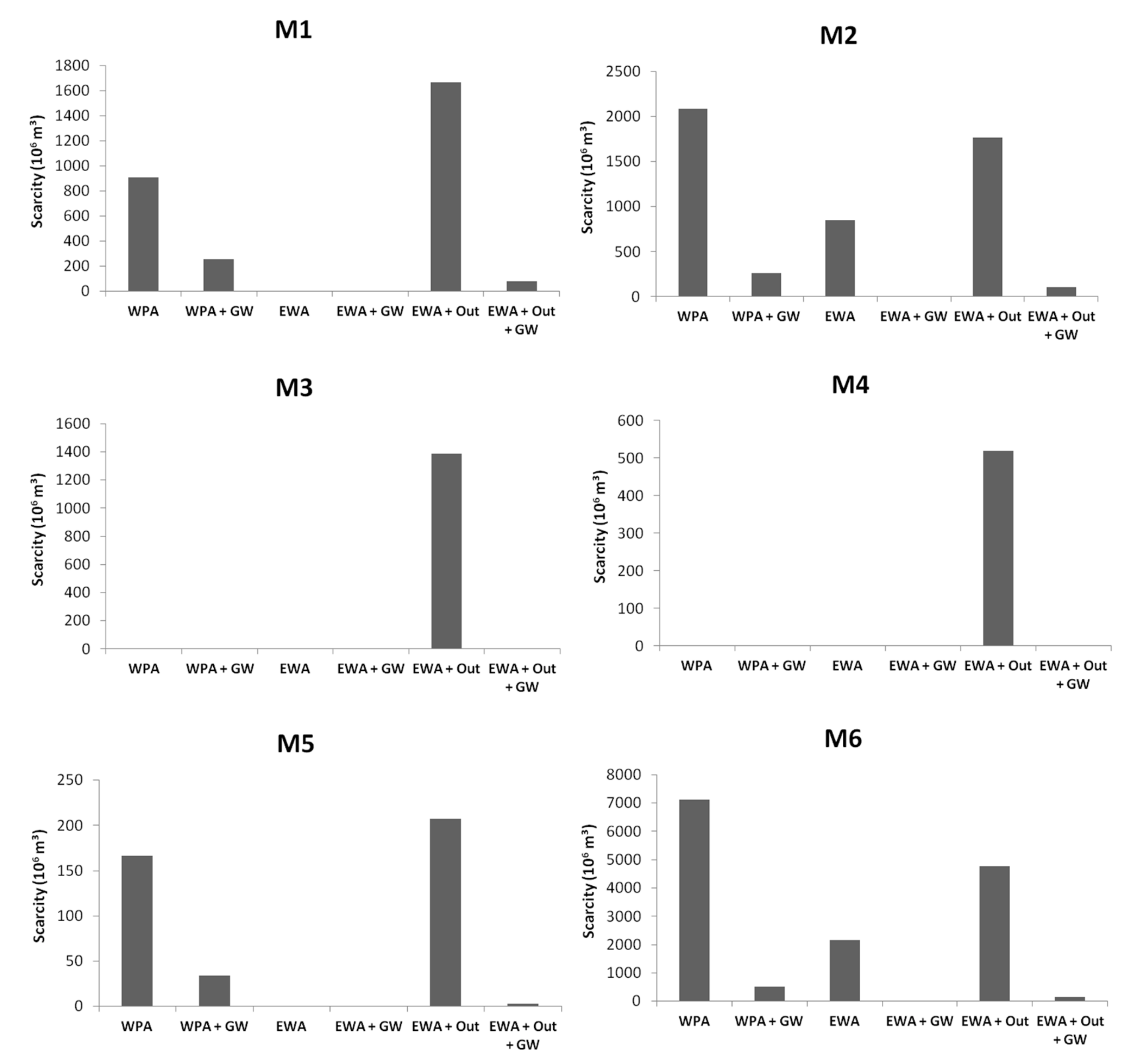
Results show that all scenarios presented some level of water scarcity, except from EWA + GW. Under the current Water Permit Allocation (WPA) scarcity was translated to a nearly accumulated R$ 2 billion in scarcity costs over 15 years, while under an Economic Water Allocation (EWA) without any constraint this figure was reduced to R$ 0.47 billion and water scarcity would be down to one third.

A proper comparison is made between WPA and EWA + Out, because both scenarios evaluate outflow restrictions; in this case, while a slight increase in the scarcity was verified (41 million m³ total in 15 years, which represents 0.4% increase), the corresponding scarcity costs were actually reduced by a total of R$ 252 million over the same period (13% decrease). These results indicate that it is possible to meet downstream water demands and reduce the scarcity cost if the current water allocation (permit based) is revised towards an economically based one.

While under the EWA scenario, the results pointed to scarcity and scarcity cost on regions M2 and M6, under the EWA + GW scenario there was no scarcity and in consequence, no scarcity cost, which was an expected result due to the increase of water availability with groundwater reserves.

Across regions the most significant values were observed on M2 and M6: these regions have the highest crop area and thus the greater water demand. Under an EWA scenario, scarcity costs could reach zero on the regions with lower water demands (M1, M3, M4 and M5); however, on M2 and M6 scarcity decreased 59% and 69% when comparing with the WPA scenario, respectively. When comparing WPA and EWA + Out, accumulated scarcity decreased 15% and 32% on regions M2 and M6, respectively. These results indicate that, with the same amount of water available (WPA and EWA + Out scenarios), there are water allocation arrangements that can increase regional economic benefit and decrease scarcity on the regions with the greatest water demands on SMRB.

By comparing the water permit allocation (WPA) with the Economic Water allocation with outflow constraint (EWA + Out) scenarios it is possible to verify that two regions (M2 and M6) presented smaller scarcity and scarcity cost in the later, while the remaining ones presented higher values than the former. Model results indicate that the regions M2 and M6 could be allocated more water and reduce their scarcity cost by R$ 712 million in 15 years, while the remaining regions would be allocated less water, causing their scarcity cost to increase by R$ 459 million in 15 years. This means the losses could be compensated by the gains with a surplus of R$ 253 million. If this value is sufficient to accommodate transaction costs and economic third-party effects (which are not evaluated here) the economic water allocation should be further investigated to improve economic efficiency in water management in the region.

3.2. Scarcity and Scarcity Cost—Seasonal Analysis

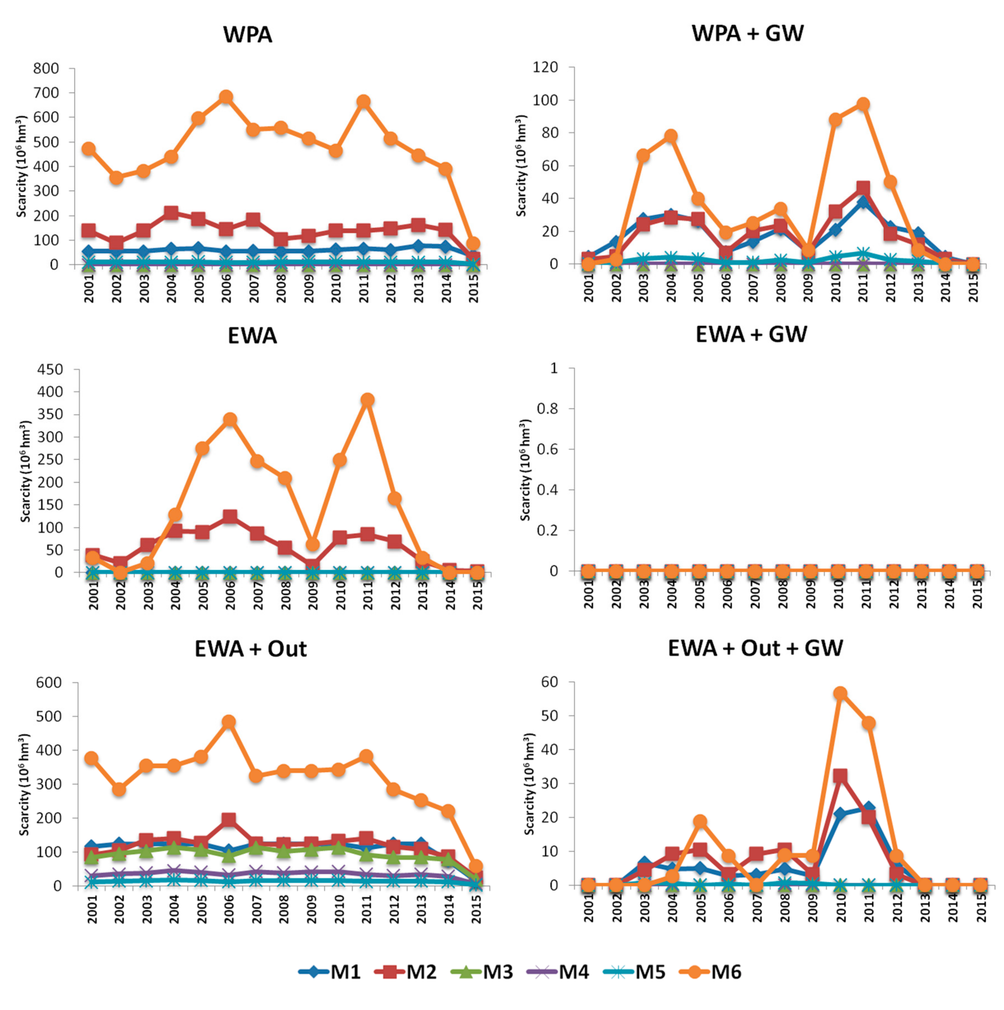
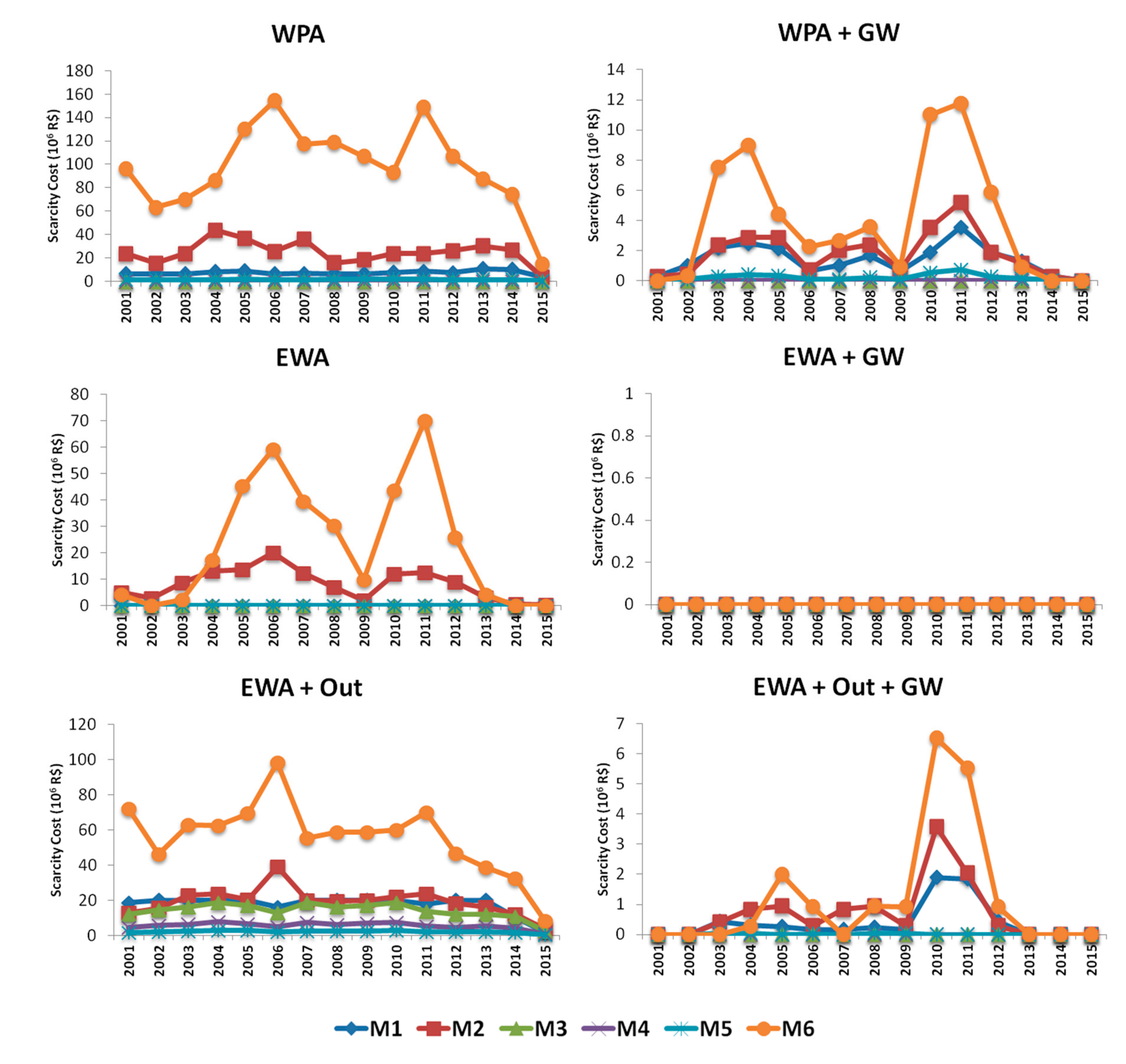
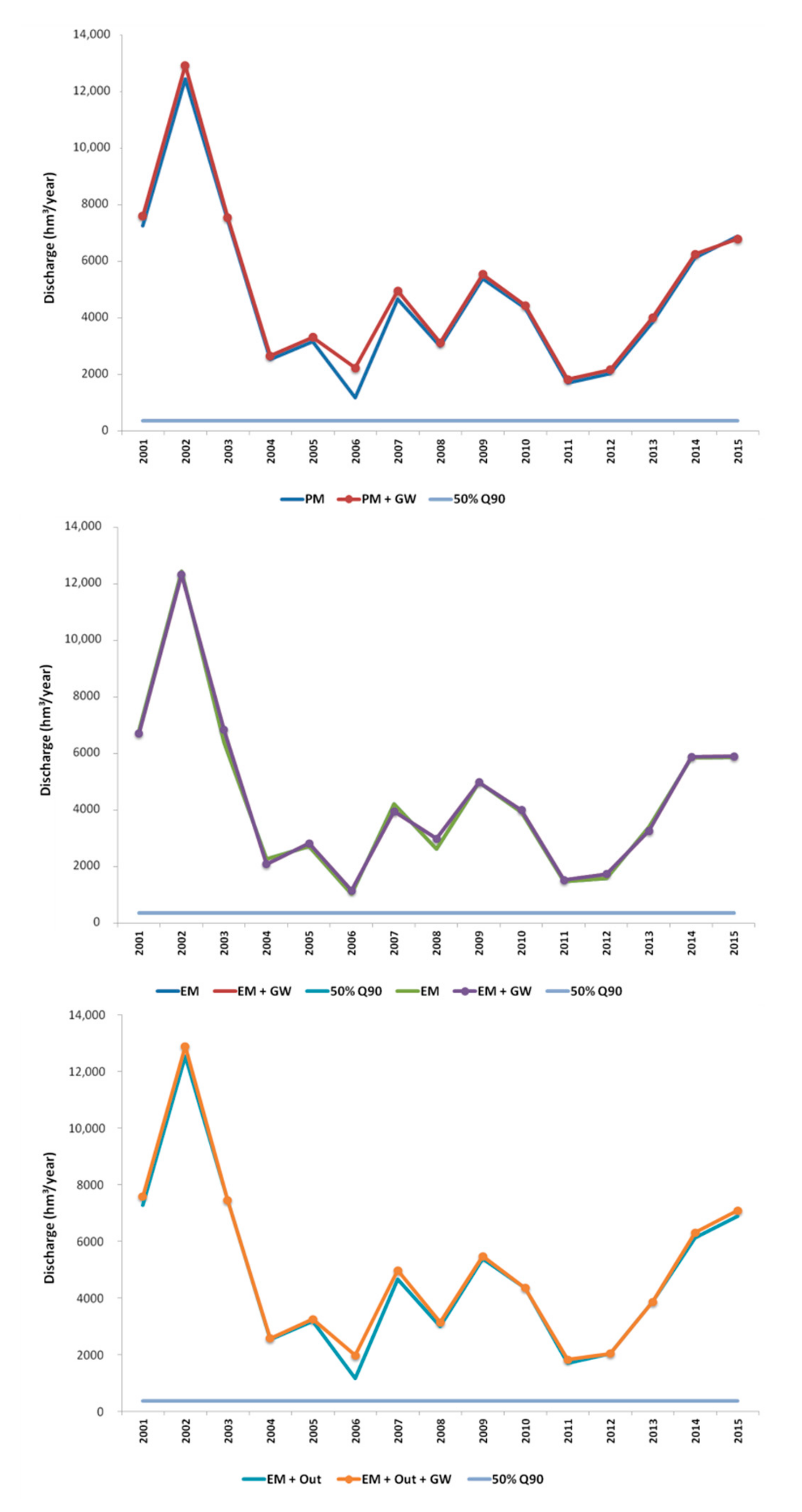
Figure 7 and Figure 8 present the evolution of scarcity and scarcity cost in all regions in each simulated scenario through the analyzed years (2001 to 2015).

It can be seen that in the years of 2006 and 2011 scarcity was higher than in other years, with larger impacts on Regions M2 and M6; with groundwater availability on WPA + GW and EWA + Out + GW results pointed to a reduction of scarcity and scarcity cost. When analyzing hydrological variables available in Reference [40] it can be seen that those years were drier than the average, mostly due to reduced precipitation; this was confirmed by the producers of the visited farms and members of the AUSM. The hydro-economic model results indicate that the availability of water from a different supply, in this case groundwater, can improve the water system’s flexibility and increase water security for its many uses.

The results obtained in this work likely overestimate the benefits, given the modeled water sources are rivers, reservoirs and groundwater but the small reservoirs on the SMRB region are also filled with runoff and this is a difficult variable to represent, because each small reservoir has a different drainage area. Although this local, small scale storage is often used in agriculture, the producers cannot always be secure about the volumes in the reservoirs, since rain prediction involves a lot of uncertainties.

As seen, scarcity and scarcity cost under an Economic Water Allocation (EWA) strategy are lower than under a Water Permit Allocation (WPA), indicating that there can be an allocation of water that generates more economic benefit to the SMRB economy. Comparing the results of the EWA strategy with the outflow restriction and the WPA strategy showed that even with the requirement to deliver an outflow to the basin downstream, there is still the possibility of allocating water more efficiently and increasing benefits. Results also showed that groundwater supplies are key to meet water demands and reduce scarcity, especially considering the proposed outflow to downstream users in the Basin Water Resources Plan. However, the groundwater use should be coordinated within the water allocation strategy.

Regions M2 and M6 presented higher vulnerability to scarcity and scarcity costs, which are the counties of São Gabriel and Dom Pedrito, which have their economies centered on agricultural production. The results of this work can be useful to show how alternative water allocation strategies and integration with groundwater can help cope with scarcity and scarcity costs under variable water supplies on the SMRB, thus increasing resilience of the water system.

3.3. GroundwaterAvailability

3.3.1. Groundwater Use Impacts on Scarcity and Scarcity Cost

When groundwater supplies are included in all scenarios, the result is a decrease in the scarcity and scarcity cost. Under the WPA strategy, the overall decrease was 90% and 94%, respectively for water scarcity and scarcity costs, while the EWA strategy decreased the same figures by 100%.

When the outflow constraint was considered, the availability of groundwater under an Economic Water Allocation allowed water scarcity to be reduced from 10,321 million m³ (15 years total) to 349 million m³, while the corresponding scarcity costs dropped from R$ 1.726 billion to R$ 34 million (15 years total). These results can be seen on Table 3 and Table 4 and Figure 5, Figure 6, Figure 7 and Figure 8.

3.3.2. Groundwater Use Analysis

Table 5. Accumulated Groundwater use on the simulations.

Accumulated Grounwater Use (106 m3)
Region	M1	M2	M3	M4	M5	M6	Total
WPA + GW	865	2293	221	88	515	6686	10,667
EWA + GW	0	901	57	0	9	2441	3409
EWA + Out + GW	4615	1879	1756	10	4	2403	10,667

shows the total use of groundwater on the three analyzed scenarios. The Water Permit Allocation strategy with groundwater (WPA + GW) and the Economic Water Allocation with restriction outflow and groundwater (EWA + Out + GW) used almost all exploitable groundwater available (which was 10,785 hm³ for the 15 years). This result highlights the usefulness of the hydro-economic optimization in exploring alternative water allocation decisions. Given the hydro-economic model objective is to decrease total scarcity cost, it searches for efficient water allocation solutions among users, which in this case pointed out to the EWA + Out + GW scenario using the same amount of groundwater as the WPA + GW but providing 69% less scarcity costs (from 111 to 34 million R$). This indicates an (economically) more effective use of available groundwater in the system.

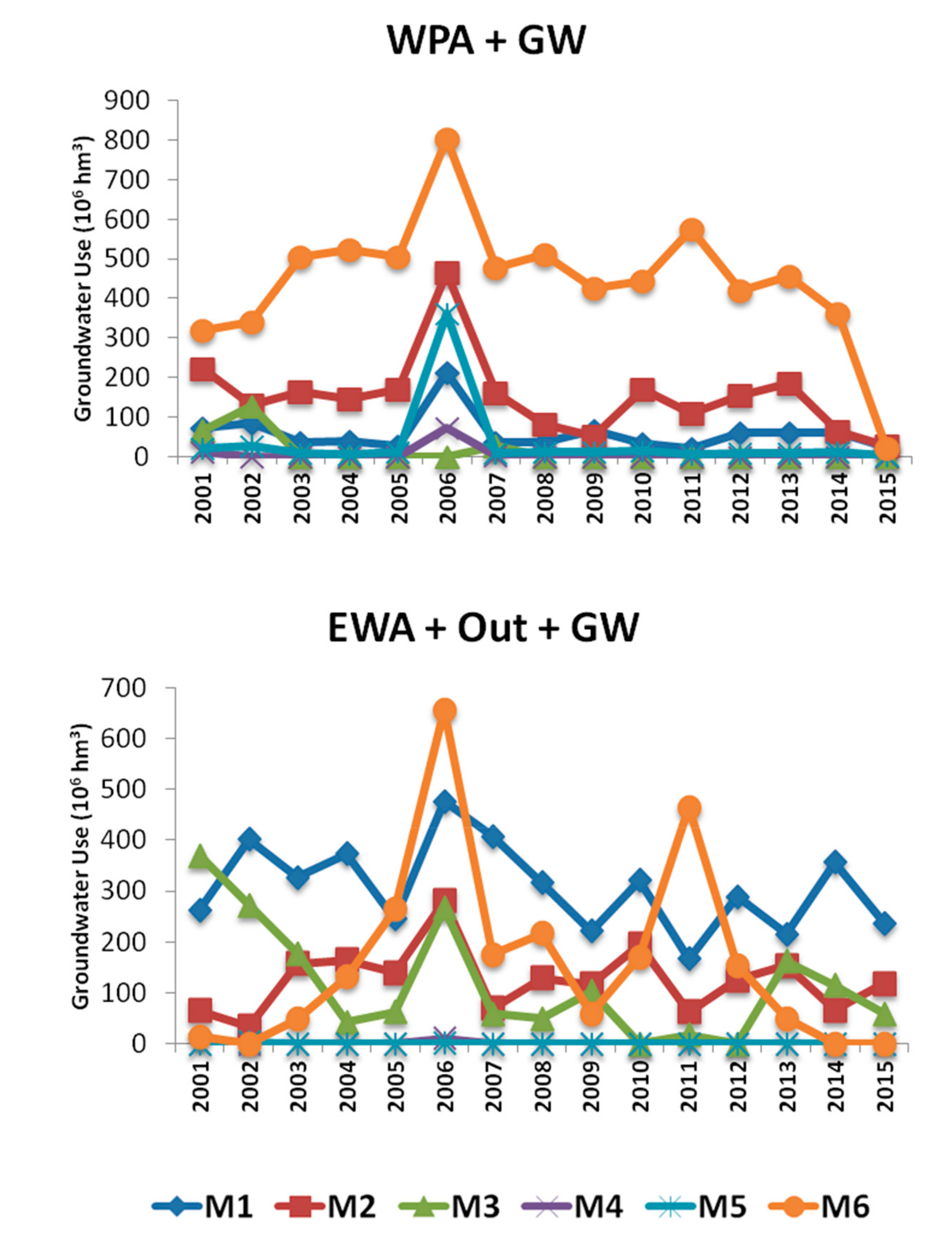
The evolution of groundwater use on these scenarios through the 15 years is shown in Figure 9. In all scenarios it can be seen the effect of the low water availability years of 2006 and 2011, especially on regions M2 and M6, which have the largest planted areas on the SMRB. Under the Water Permit Allocation with groundwater (WPA + GW) scenario, groundwater is used according to the water demands, limited by the water permits in each region, while under the Economically Water Allocation (EWA + Out + GW) scenario water is allocated to reduce scarcity costs but restricted only to the outflow to the downstream basin. This explains their different behaviors along the years. (WPA + GW) had to fulfill the permits while (EWA + Out + GW) could allocate water across the different regions and water supply sources, resulting in the use of groundwater on regions M2 and M6, which have the largest scarcity among all regions.

These results can indicate a strategy for the conjunctive use of surface water and groundwater: for the SMRB case, the period with the lowest water availability matches with the highest water demand for irrigation and so groundwater could be used on this time of the year to increase water availability and reduce economic losses, taking the pressure off surface water supplies. Geographically, there is also a shift in the groundwater use from M6 to M1 and to M3 (comparing WPA + GW with EWA + Out + GW). This result could be useful in future decisions to allocate groundwater permits, integrated with surface water.

3.4. Downstream Outflow Analysis

Figure 10 shows a comparison between the outflows on all simulated scenarios with the limited outflow (50% of the Q90). It can be seen that all simulated scenarios delivery more water than the minimum to the downstream basin, thus being in conformance with the restriction proposed on the Basin Management Plan.

When comparing the outflow of scenarios with and without the groundwater use, it can be seen that models with groundwater availability have higher outflow than the respective scenario without groundwater: (WPA + GW) deliveries 9% more outflow than WPA and (EWA + Out + GW) deliveries 7% more than (EWA + Out). These results show that integrating groundwater use into water allocation decisions is a must for effective water resources management in that basin. For example, if the downstream users require more water in the near future, groundwater supplies can bring in much needed flexibility to accommodate those demands without resorting to conflict and to the benefit of both basins, provided the use of these supplies is integrated to a broader water allocation strategy, as investigated in this paper.

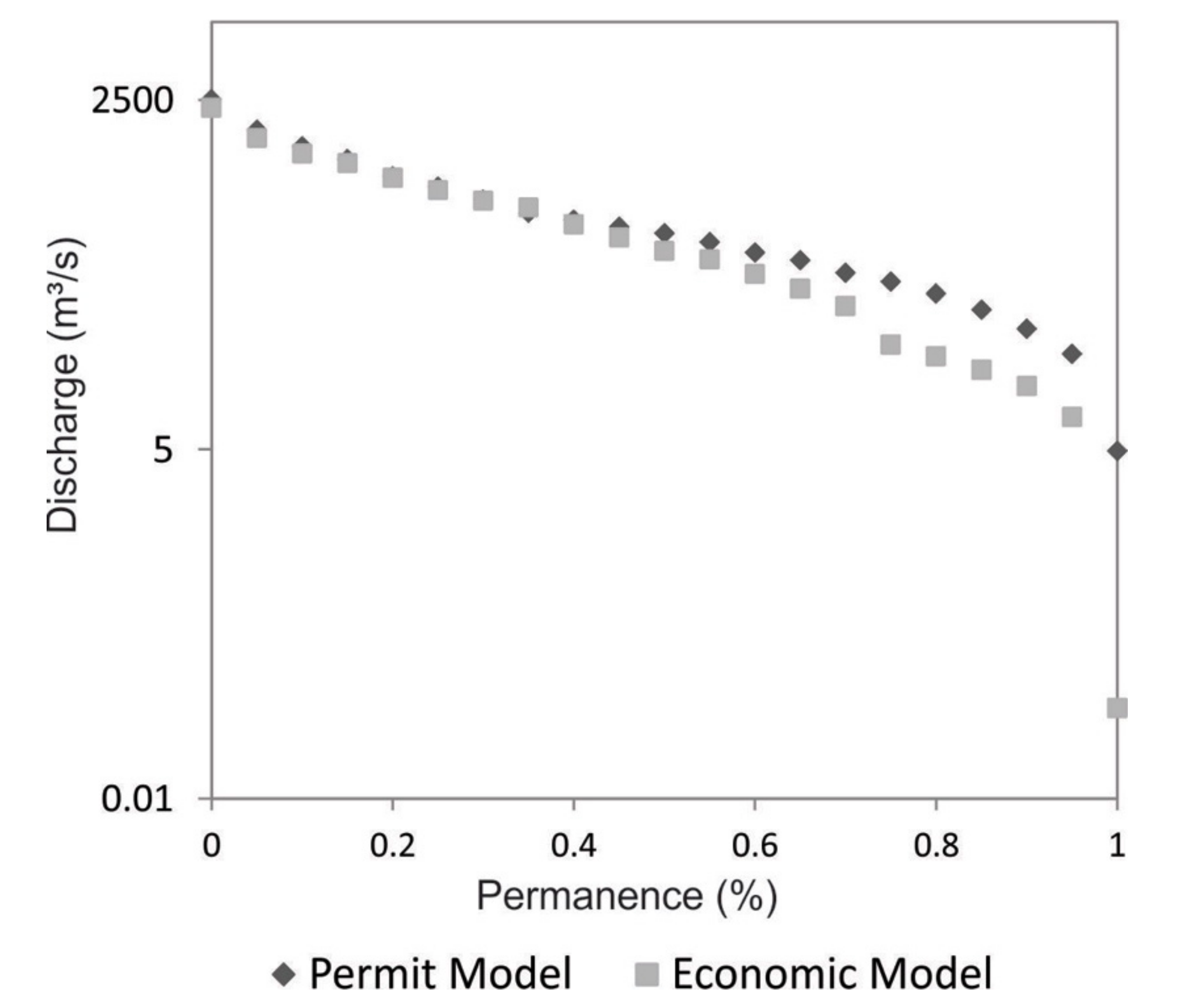
Figure 11 compares the flow duration curves for the outflows to the downstream users (Ibicuí River) under the Economic Water Allocation strategy (EWA) and the Water Permit Allocation (WPA) strategy. As seen, the outflow under EWA is lower than that under the WPA outflow on lower discharge values, suggesting that in low water availability periods, an economically driven water allocation strategy would deliver less water to the downstream basin. This result is important as it provides a basis for negotiations between the two basins, including the establishment of compensation mechanisms or agreements for mutual benefit. A more detailed outflow comparison is presented later in this paper.

3.5. The Role of Water Management

The results indicate how water scarcity and economic losses can be reduced by having different water sources and infrastructures that allow integrated management. Under economically driven water allocation strategies, some regions would face increased water scarcity while the others would perceive the opposite. However, the sum of the economic benefit in all regions was bigger than the sum of the economic losses. While the use of groundwater would reduce scarcity costs across the entire region, some of the SMRB agricultural producers could be further adjusted by changing the crop mix between regions, even though some regions would still experience overall increased scarcity costs. In such cases, the Water Management Authority and the Watershed Committee should work together to (a) negotiate alternative water allocation strategies and economic compensation mechanisms, for example the implementation of water markets as in Southern California [9] in the United States and Jucar Basin in Spain [51] and (b) develop and apply economic water management instruments to signal water scarcity to users and motivate rational use. Those are important elements for water management to effectively increase efficiency and economic benefits when facing low water availability. This situation is captured by the term opportunity cost, which is the value of the next best selection that could have been undertaken [25], which means the economic benefit generated by allocating water from one use to a higher value one use.

Among economic water management instruments, water charges could have different values depending on the water supply source (e.g., groundwater, reservoirs, rivers) and depending on its use (e.g., type of culture, industry). That would enable the watershed committee to actively propose and negotiate instruments that would be effective in inducing producers’ decisions, reducing scarcity cost and improving economic development on the Basin. This strategy is foreseen on the Santa Maria River Basin Water Resources Plan, where the Watershed committee defined guidelines that involve different prices for water charging. However, existing guidelines still lack a better understanding of (a) the economic value to the water to users and (b) scarcity costs across the watershed, which are provided in this paper.

4. Conclusions

In water systems with significant competitive uses and hydrology variability, water scarcity may be unavoidable. It is up to the water management to improve instruments and to provide the necessary framework so that arrangements and negotiations among users can take place to mitigate scarcity and scarcity costs.

In water systems where water rights are established by a water permit system, such as the case studied here, the procedure to issue the water permits may lack a broader economic view of the watershed, yielding a water allocation that misses valuable opportunities to reduce scarcity costs. By comparing the current water allocation system in the study watershed (based on water permits) with an alternative that is economically based, some key conclusions and insights are drawn:

• It is possible to reduce, but not entirely eliminate, water scarcity and scarcity costs in the basin through some reallocation of water between users.
• It is possible to meet downstream water demands at a lower cost if the current water allocation (permit based) is revised towards an economically based one. This is an important result to support future negotiations among users and avoid conflict;
• Groundwater has a high potential as a component to reduce scarcity and costs and this potential can be significantly boosted when its use is integrated with surface supplies and economically allocated;
• Finally, under an economically based water allocation, there could be enough benefits (in terms of reduced scarcity costs during drought events) capable of compensating other users for water reallocation. While we still cannot tell if such operations should be carried out, given transaction costs and third party impacts were not accessed, this result indicates that it is a possibility worthy of further consideration.