An Improved Genetic Algorithm for Optimal Layout of Flow Meters and Valves in Water Network Partitioning

Abstract

The paradigm of “divide and conquer” has been well used in Water Distribution Systems (WDSs) zoning planning in recent years. Indeed, Water Network Partitioning (WNP) has played an irreplaceable role in leakage control and pressure management; meanwhile it also has certain drawbacks, such as reduction of the supply reliability of the pipe network system and increased terminal dead water, as a result of the closure of the pipe section. In this paper, an improvement is made to the method proposed by Di Nardo et al. (2013) for optimal location of flow meters and valves. Three improvements to the genetic algorithm are proposed in this work for better and faster optimization in the dividing phase of WNP: preliminary hydraulic analysis which reduces the number of decision variables; modifications to the crossover mechanism to protect the superior individuals in the later stage; and boundary pipe grouping and mutation based on the pipe importance. The objective function considers the master–subordinate relationship when minimizing the number of flow meters and the difference of hydraulic state compared to original WDS. Another objective function of minimizing the deterioration of water quality compared to original WDS is also evaluated. The proposed method is applied for the WNP in a real WDS. Results show that it plays an effective role in the optimization of layout of the flow meters and valves in WNP.

1. Introduction

As one of the most crucial municipal infrastructures, Water Distribution Systems (WDSs) play an irreplaceable role in social and economic development. In older design philosophy of WDSs, we blindly pursued greater pipe redundancy (i.e., complicated looped system) to enhance the system’s ability to protect against potential risks (e.g., pipe bursts or fire demand). There was no doubt that it brought higher reliability of supply service but meanwhile we cannot ignore the management inconvenience, especially the difficulty of water loss evaluation in such a complicated WDS, resulting in failure to detect leaks and pipe bursts in time, which were extremely harmful to the sustainable development of the social ecology [1].

Consequently, in recent years, researchers around the world have focused on finding a new approach aimed at simplifying the management of WDSs. The paradigm of “divide and conquer” was hence vigorously promoted, along with a new management model of WDSs, called District Metered Areas (DMAs), which can significantly improve the management level through real-time monitoring of inlet and outlet flows in each subsystem (i.e., water balance analysis); certainly, DMAs play broader roles than water metering. The creation of DMAs can also help the implementation of pressure management [2] with the use of Pressure-Reducing Valves (PRVs), allowing a low level of leakage to be kept in the whole network system; additionally, replacing the PRVs with PATs (Pumps as Turbines) in the water distribution network has proven to be useful for energy recovery [3,4], which has huge application prospects in the future. Furthermore, some studies have shown that the division of DMAs do have a function of protecting the system from water contamination [5] and a better detection of pipe bursting [6].

The two main issues of DMA design are how to shape and dimension the network sub-zones (clustering phase) and where to locate meters and gate valves (dividing phase). Presently, considerable theoretical methods can be used in the clustering phase of DMA design and divide into four categories: graph theory algorithm [7,8,9,10], cluster analysis [11,12,13], community structure [14,15,16,17], and multi-agent algorithm [18,19,20]. The graph theory algorithm is first introduced to solve the WNP problems by Tzatchkov et al. [7]. They used breadth-first search (BFS) and depth-first (DFS) algorithms to find feasible partitioning solutions, and later many graph theoretic heuristic techniques were combined to better address the problems, such as Dijkstra’s shortest path algorithm [9] and recursive bisection method [21], but sometimes this method cannot effectively control the number of boundary pipes, resulting in an increase in investment costs; Cluster analysis is a traditionally used method in WDS; the similarity between nodes is used to cluster the sub-zones. Perelman et al. [22] used a bottom-up hierarchical clustering algorithm, which, based on the Euclidean distance between nodes, partitioned the whole network; however, since the Euclidean distance measure does not consider the connectivity of nodes, the internal connectivity of each cluster should be verified; and lately a spectral clustering algorithm [11,12] was widely applied in the WNP issues because of its reliability in minimizing the number of edge-cuts and balancing the number of nodes for each district. Diao et al. [15] first applied the community structure algorithm, based on the concept of ‘modularity’ to detect the group characteristics of the WDS. This method is also widely used due to its high speed and reliability in decomposition of large-scale, complex systems [23], but the balance between DMAs is not so well, and an improved version of this method is proposed by Giustolisi and Ridolfi [24] which considers the attributes of nodes and pipes. A comprehensive comparison of the methods described above was done by Sela Perelman et al. [22] and Di Nardo et al. [17].

The DMA boundary pipes are determined after the clustering phase, and then the layout of the flow meters (i.e., open pipes) and gate valves (i.e., closed pipes) among the boundary pipes is optimized in the dividing phase to minimize the number of flow meters or the hydraulic performance deterioration [25,26], etc. Simulated Annealing algorithm [27], iterative method [12,15,16], and single-objective or multi-objective optimization based on economic [25], energy and water quality [28,29] issues can be used in this phase. The iterative method is a simple method that suitable for all sizes of WDS [15]. Through the initial analysis of the importance of each pipe (according to diameter or flow rate, etc.), the least important pipe is iteratively closed until normal hydraulic conditions cannot be met. At this point the number of flow meters reaches the minimum. The iterative method is still an empirical method in essence, and it cannot consider the joint effect caused by simultaneous closure of multiple pipes, so there is a certain gap between the results and those obtained by the heuristic algorithm [30]. The heuristic algorithms globally search the layout of the flow meter and valve position based on the hydraulic performance of the water distribution network. However, the heuristic algorithm also has its own drawback, i.e., when the number of decision variables increases, the convergence efficiency drops significantly because the search space grows exponentially.

In this study, the main work is done to improve the optimization performance and efficiency of the genetic algorithm (GA) in the dividing phase of WNP, which consists of selection, crossover, and mutation operations, developed by Goldberg et al. [31]. The contributions of this work are listed below: 1) Changing the dual-objective problem to a single-objective problem by considering the master–subordinate relationship of the two objective function, which improved the computational efficiency; 2) Three improvements integrated in the GA, including preliminary analysis of boundary pipes, modified crossover and mutation mechanism, and the case study verified the superiority of this strategy, especially in terms of stability of output and convergence speed. The objective functions to consider the network resilience and the water quality impact caused by WDS partition were tested independently. As a result, a high similarity in the locations of flow meters and gate valves for these two objective functions are found.

2. Methodology

The framework of the whole partitioning methodology is shown in Figure 1. In the clustering stage, a modularity-based algorithm [32] is applied to deal with the problem of sectorization, and the adjacency matrix A_ij of topology structure and total number of pipes m is needed as initial parameters; then the GA is used in the optimization procedure of the dividing stage.

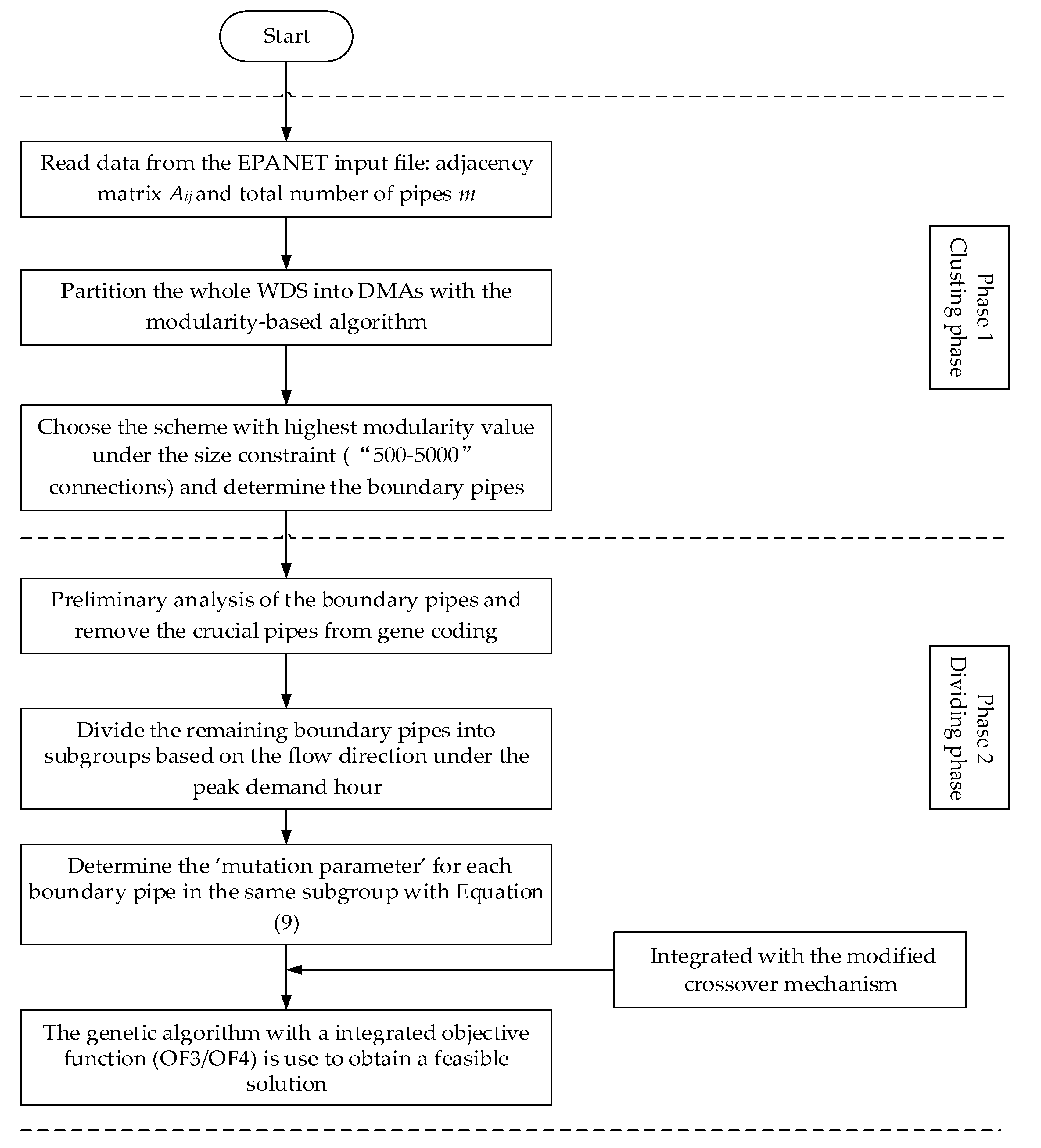
2.1. Network Clustering

Similar to many physical and social processes (e.g., business and academic circles) in the world, a water distribution system can also be naturally characterized by a simple topological graph G = G(V,E), where V represents n nodes (consumers, sources, and tanks) and E represents m edges (pipes, valves, and pumps) in a WDS. The approach adopted in this phase owns a bottom-up merge process and is based on the concept of ‘modularity’, which can quantify the quality of WDS partition [23,32,33], called the Fast-Newman algorithm. The modularity Q is expressed in Equation (1), and Q ≥ 0.3 indicates a good division into communities [16].

$$Q=\frac{1}{2m}{{\displaystyle \sum }}_{vw}\left(A_{vw}-\frac{k_v{k}_w}{2m}\right)\delta \left(c_v,c_w\right) Q\in \left[-0.5,1\right)$$

(1)

where m represents the total number of links in the network; v and w are vertexes indexes; k_v (k_w) is the sum of the number of edges connected to vertex v (w); A_vw = 1 if there is a link connecting the vertexes v and w; A_vw = 0 otherwise; c_v, c_w is the communities which the vertexes v and w belong to; δ(c_v,c_w ) = 1 if vertexes v and w are in the same community, 0 otherwise. The brief steps of the algorithm are described below:

• At first each node represents a community, and the initial modularity is calculated with Equation (1).
• Evaluate the modularity change $\Delta Q_{vw}$ for each pair of communities v and w with Equation (2), assuming they are combined.
• Merge the pair of communities v* and w* with max ($\Delta Q_{vw}$) (could be negative value) and the modularity of the current structure equals the modularity of the previous structure plus max ($\Delta Q_{vw}$).
• Step 2 and 3 is repeated until all the nodes merged into one community.

$$\Delta Q_{vw}=\{\begin{array}{cc}\hfill \frac{1}{2m}-\frac{k_v{k}_w}{{\left(2m\right)}^2},& \mathrm{if} v,w \mathrm{are} \mathrm{connected}\hfill \\ \hfill 0 ,& \mathrm{otherwise}\hfill \end{array}$$

(2)

The partition scheme with highest Q value represents its sub-systems that have stronger internal than external connections, but is not necessarily the best solution because the DMA size needs to be controlled between 500–5000 customer connections according to the guidelines [34]. It becomes much more difficult to control water losses and locate the new bursts when a DMA contains more than 5000 customers [27]; meanwhile more investment will be spent if the size of DMA is too small. Therefore, what we indeed need is the scheme with highest Q value given the premise of satisfying the size constraint. More detail about the Fast-Newman algorithm can be found in previous literature [15,24].

2.2. Network Dividing

For the dividing stage of WNP (Water Network Partitioning), Di Nardo et al. [25] proposed a method based on GA with the following objective function, to protect the hydraulic performance of the original system as much as possible:

$$OF1=max\left(P_D=\gamma {\displaystyle \sum }_{i=1}^n{Q}_i{H}_i\right)$$

(3)

where γ is the specific weight of water, Q_i and H_i are the water demand and head at each network node, and P_D is the total node power of the network. Generally, partitioning schemes with more flow meters (i.e., closing fewer pipes) would have a higher objective value P_D, hence the optimal solution is the case that all the boundary pipes are installed with flow meters (i.e., remain open). However, it is not the answer we truly need as more flow meters lead to a less convenient management and higher cost. Therefore Di Nardo et al. [25] tried to solve the above problem by determining the number of flow meters in advance, but it is difficult to decide how many flow meters should be installed as a trade-off between the hydraulic performance and cost, especially for large-scale WDN. Therefore, the number of flow meters should be considered to be one of the objective functions instead of being a predetermined value. Thus, it forms a dual-objective problem as Equation (4):

$$OF2=\{\begin{array}{c}min\left(N_{fm}\right)\\ max\left(P_D\right)\end{array}$$

(4)

At this point, the NSGA-II algorithm [35] is generally used to optimize this dual-objective problem. It is feasible but not the optimal selection—in the previous literature, almost all researchers agree that the number of flow meters should be reduced as much as possible in the dividing phase of WNP under the premise of meeting normal hydraulic conditions (i.e., all demand nodes should meet the minimum service pressure) [15,16]. If possible, the best solution would be each district own just one single inflow meter [25], because fewer flow meters can not only simplify the calculation of the synchronous water balance and improve the reliability of flow monitoring, but also reduce the costs of initial investment and later operation and maintenance costs. Therefore, we would like the second objective function in Equation (4) to be subjected to the first one; in other words, we would give the priority to the choice of the scheme with fewer flow meters, and then consider the role of the second objective function. However, the NSGA-II algorithm cannot embody this relationship between the two objective functions, resulting in a lot of time wasted on optimizing solutions (Pareto frontier).

To address above problem, this paper proposes a new objective function form shown in Equation (5), which can not only combine the two objective functions together, but also embodies the primary and secondary relations of the two objective functions. The purpose of the first term is to minimize the number of flow meters (its value is an integer) and the second term is to search the solution that has less impact on the hydraulic performance compared to original WDN. The value of the second term is between 0 and 1, ensuring that the latter one is subject to the former one.

$$OF3=min\left(N_{fm}+\frac{P_{D0}-P_D}{P_{D0}}\right)$$

(5)

where N_fm is the number of flow meters, P_D0 is the total node power of the network before WNP and P_D is the total node power after WNP.

The fitness function, Equation (6), is obtained using the boundary construction method, by changing the minimum optimization into the maximum optimization, and the fitness value can be ensured larger than zero.

$$Fit=N_p-OF3=N_p-N_{fm}-\frac{P_{D0}-P_D}{P_{D0}}=N_{gv}-\frac{P_{D0}-P_D}{P_{D0}}$$

(6)

where N_p is the number of boundary pipes, N_gv represents the number of gate valves

To adjust the selective pressure effectively, a rank-based fitness assignment method [36,37] is adopted to better distinguish the fitness between individuals, especially in the later stage of optimization. The specific fitness assignment function is shown in Equation (7)

$$Fit\left(i\right)=2-SP+\frac{2\left(SP-1\right)\left(i-1\right)}{n-1}, SPϵ\left[1.0,2.0\right]$$

(7)

where i is the rank of an individual in the population, SP is the selection pressure and set SP = 1.5 in this work, and n is the size of the population. A simple example (the population size n adopts 5) is given to better understand the role of the rank-based fitness assignment method in this work as shown in

Table 1. A simple example of rank-based fitness assignment method.

Individual Index	Real Fitness Value		Individual Index	Real Fitness Value	Rank		Individual Index	Assigned Fitness Value
1	27.97325	sort	4	27.93649	1	assign	4	0.5
2	28.96611		1	27.97325	2		1	0.75
3	28.94224		3	28.94224	3		3	1.0
4	27.93649		5	28.95028	4		5	1.25
5	28.95028		2	28.96611	5		2	1.5

. The real fitness values are firstly calculated with Equation (6), then rank the individuals in the following way: the best one has rank n and the worst one has rank 1.

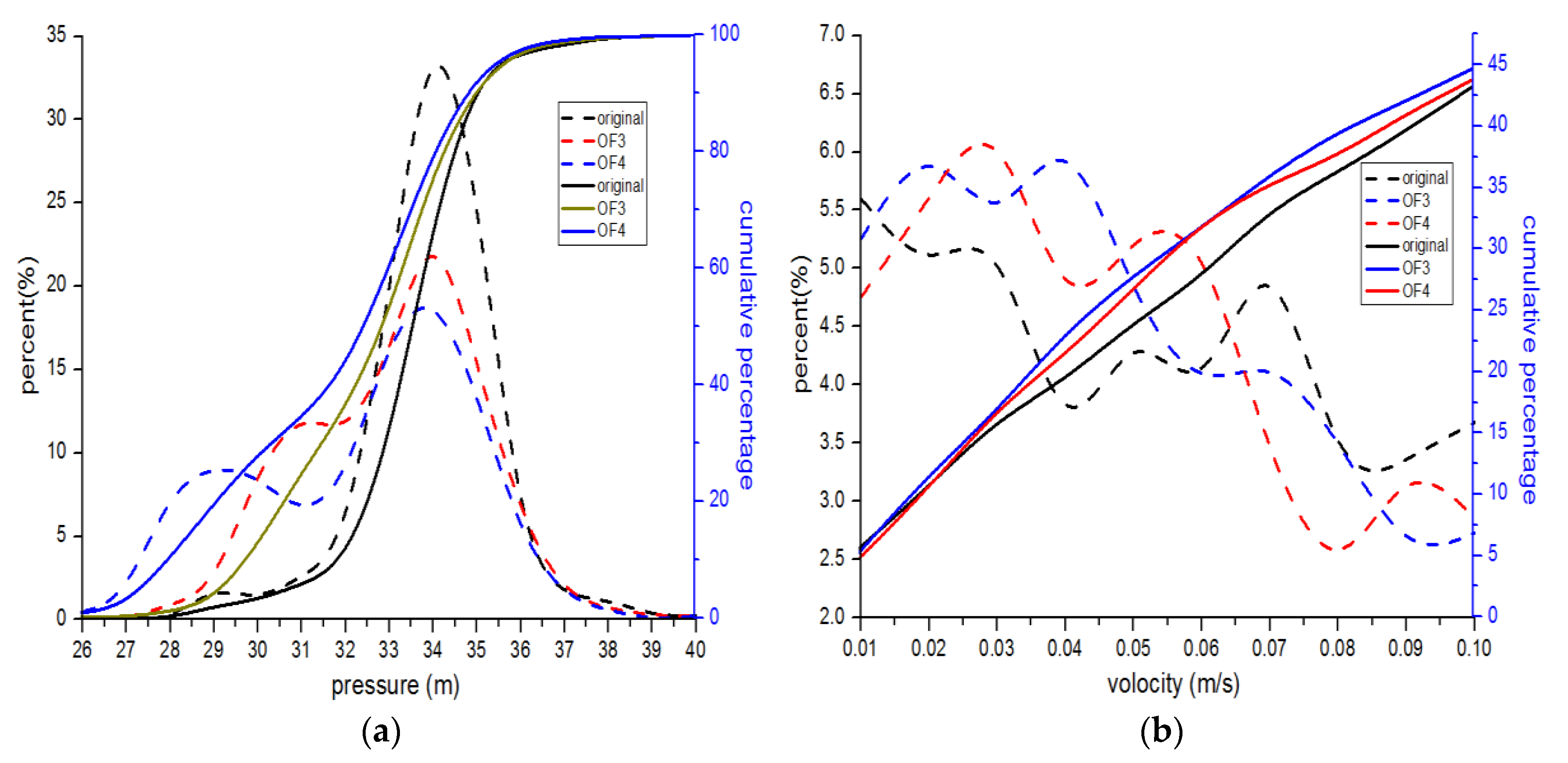
Another objective function is adopted in this paper which considers minimizing the deterioration of water quality caused by WNP. The water velocity of pipes is used as an indicator to evaluate the water quality change before and after WNP. Giving the objective function in Equation (8).

$$OF4=min\left(N_{fm}+\frac{{{\displaystyle \sum }}_{i=1}^{p}V{O}_i\Delta v_i\delta \left(m_1,m_2\right)}{{{\displaystyle \sum }}_{i=1}^{p}V{O}_i{v}_i}\right)$$

(8)

where p is the number of pipes; VO is the pipe volume; v is the pipe velocity before WDP; m₁ representing the event that the pipe velocity after WDP is lower than before, m₂ representing the event that the pipe velocity after WDP is lower than 0.1 m/s, and δ (m₁, m₂) = 1 if both events m₁ and m₂ are true at the same time, 0 otherwise; △v_i is the flow velocity difference before and after WNP.

2.3. Improvements for Better Optimization

The binary coding is used to encode the chromosomes (i.e., individual), one chromosome is composed of a sequence of genes. Gene i assumes 0 if a flow meter installed in i-th pipe; otherwise, the value is 1 if a gate valve installed. As mentioned by other scholars, the efficiency of GA is obviously affected by the number of decision variables (i.e., boundary pipes) in the optimization process of dividing phase [15]. There are two main reasons: first, the increasing number of decision variables inevitably leads to an exponential growth in search space, significantly affecting the optimization efficiency and making the entire optimization process more time-consuming. Second, binary coding cannot truly reflect the relationship between genes [38], which are not really independent of each other (e.g., for a DMA without water source, all the boundary pipes connecting it cannot be closed at the same time otherwise no water will be supplied in this area). Moreover, the common crossover mechanism has great damage to individuals especially for those superior individuals in the later stage of optimization because of the direct break of chromosomes, though in the earlier stage it helps to maintain the diversity of the population. This drawback becomes more apparent when the length of the chromosome increases. To address the above-mentioned issue, three improvements are proposed in this work

Step 1: Reduce the number of decision variables through preliminary analysis

In fact, there are several pipes among the boundary pipes that are not necessary to participate in gene coding, because the closure of any one of them will result in local pressure deficit or even water supply disruption (e. g. main water transmission pipes or a unique inflow pipe for one specific DMA). The gene points corresponding to those pipes must be installed with flow meters can hence be deleted from the chromosome. In this way, the search space is greatly reduced.

The specific method in the procedure is as follows: Each time close one boundary pipe (all other boundary pipes should be open except the selected one) and then run the hydraulic simulation to find the pipes where the minimum pressure is lower than the normal service pressure, i.e., this boundary pipe must be opened to satisfy the minimum pressure and can be removed from the decision variables (the chromosome). All the pipes to be removed from the chromosome can be found by repeating this procedure for all the boundary pipes.

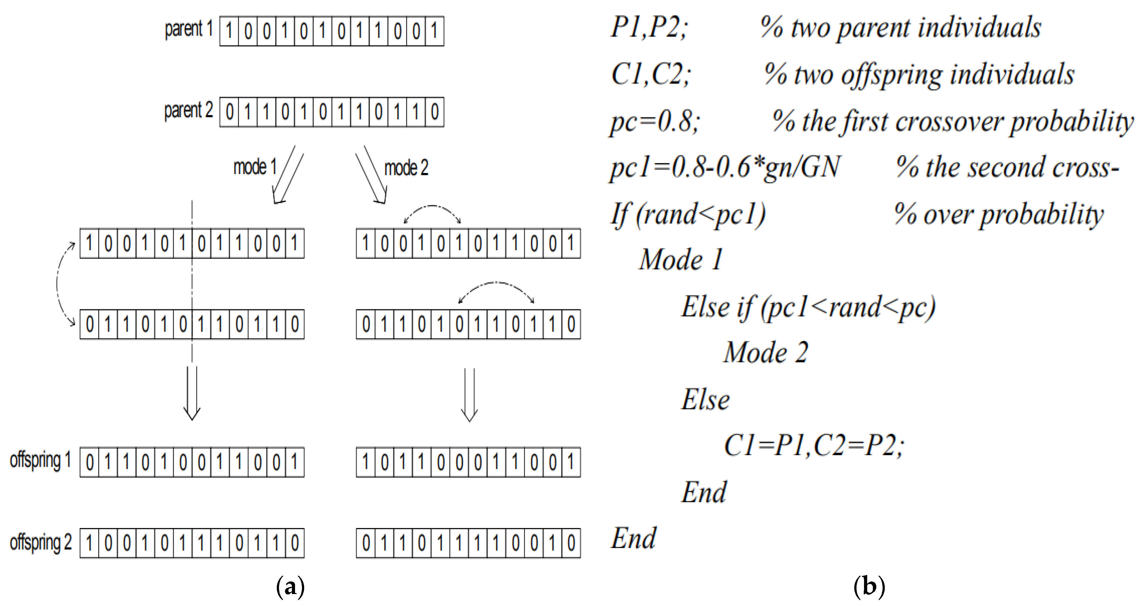
Step 2: Modify the crossover mechanism

A new crossover mechanism is proposed to better protect the individuals in the later stages of optimization; at the same time, it enhances the local search ability of the algorithm. The pseudo-code of new crossover mechanism is described in Figure 2b, where gn represents the current generation, GN represents the total operation generations which should be determined in advance, pc is the first crossover probability with a fixed value of 0.8 meanwhile pc1 is the second crossover probability, which is related to the current generation gn. As shown in Figure 2a, mode 1 is the traditional crossover method meanwhile mode 2 is a new crossover method that exchanges the positions of two gene points, one coded 1, another coded 0; both of them are randomly selected (the physical meaning is to change the location of one randomly chosen flow meter meanwhile the total number of flow meters remains unchanged). As the generation (i.e., gn) increases, the probability of the mode 1 becomes smaller and the mode 2 becomes larger because of the declining value of pc1. The crossover method of mode 2 can better prevent the superior individuals not being damaged.

Step 3: Improve the mutation parameter

Through assigning ‘mutation parameter’ to each gene point, the importance level of each boundary pipe can hence be embodied and mutually distinguished in the optimization procedure, effectively accelerating the convergence velocity. At the same time, it will not lose the ability to search for potentially better solution such as the iterative method because of the absolute ordering relationship.

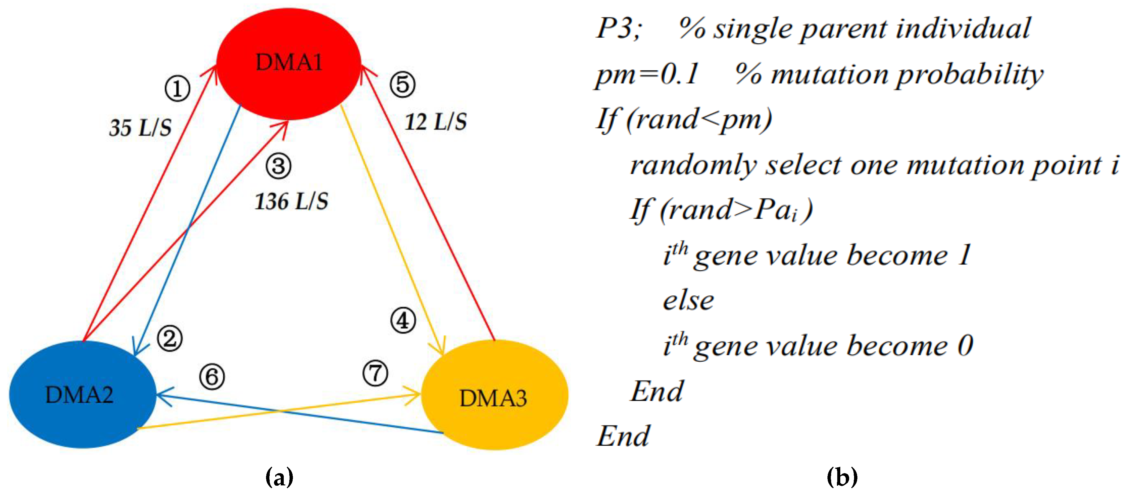
The boundary pipes are first divided into subgroups based on the flow direction under the peak demand hour. To better illustrate the method, an example is shown in Figure 3a; pipe 1, 3, 5 are classified together because they are all the inflow pipes belonging to DMA1 and pipe 2, 6 are grouped together likewise. The pipes classified in the same subgroup play an identical role in the WDS (i.e., supply water for the same DMA), hence they are substitutes for each other and can be classified together for comparison to show the distinction in importance.

Then we determine the ‘mutation parameter’ for each boundary pipe according to Equation (9). Taking Figure 3a as an example, for DMA1, the flow rates of three inflow pipes 1, 3, 5 are 35 L/s, 136 L/s, 12 L/s respectively, and the corresponding ‘mutation parameters’ are 0.4290, 0.7049, 0.3661 as calculated by Equation (9).

$$P{a}_{i,j}=0.5+\frac{0.5\left(Q_{i,j}-Mea{n}_i\right)}{Su{m}_i}$$

(9)

where Pa_i,j is the ‘mutation parameter’ of jth pipe in ith group; Q_i,j is the flow rate of jth pipe in ith group; Mean_i is the average flow rate of ith group; Sum_i is the sum of the flow rate of all pipes in ith group. The 0.5 in Equation (9) means the boundary pipes have the same possibility to install flow meters or gate valves if we do not consider any hydraulic characteristics, and the second term in RHS of Equation (9) considers their hydraulic importance (the 0.5 in the second term ensures Pa_i,j less than 1).

As we can see, the more important pipe owns larger values of ‘mutation parameter’ such that it has greater possibility of being an inflow pipe with the flow meter installed (Figure 3b shows the pseudo-code). Taking pipe 3 as an example, it is the most important one of the three and owns the highest value 0.7049. Then, when its corresponding gene point is selected as the mutation point, if a randomly generated number (ranging from 0 to 1) is greater than 0.7049, the gene value becomes 1 (i.e., install the valve), otherwise it becomes 0 (i.e., install the flow meter). In this way the more important pipe has a larger opportunity to become an inflow pipe outside of being closed.

3. Results and Discussion

We test the proposed methodology in a medium-size water distribution system located in southern China, H Town [39], which owns one fixed-head reservoir, 898 demand nodes, and 1012 pipes. Under the peak hour demand scenario, a minimum service pressure of 24 m is required-more details can be referred to

Table 2. Characteristics of H town.

Property	Value
Number of Nodes	898
Number of Pipes	1012
Number of Reservoirs	1
Total pipe length	518.02 km
Total water demand	1498.9 L/s
Total connections	42826
Average water demand	0.032 L/s/connection

.

In the clustering stage of WNP, the Fast-Newman algorithm is used to create the sub-zones (results shown in Figure 4). The characteristics of DMAs are shown in

Table 3. Characteristics of H town’s DMAs.

DMA Index	Number of Nodes	Water Demand (L/s)	Equivalent Connections
1	48	64.72	1849
2	83	133.94	3827
3	50	98.09	2803
4	50	158.02	4515
5	85	118.71	3392
6	35	60.22	1721
7	53	88.04	2515
8	76	165.33	4724
9	67	143.32	4095
10	40	41.69	1191
11	50	93.42	2669
12	67	48.86	1396
13	77	57.86	1653
14	62	85.6	2446
15	56	140.96	4027

. All DMAs satisfy the size constraint mentioned above and the value of modularity Q is 0.713, a fairly high value because of the relatively obvious community characteristics the WDS owns.

After the above procedure, a set of boundary pipes containing 48 pipes (corresponding to 48 decision variables) is obtained, and then the layout of the flow meters and gate valves among these boundary pipes is optimized using GA with objective function OF3 (a population of 50 individuals, 200 generations, Pcorss = 0.8, Pmut = 0.1). Hydraulic simulation is carried out during the peak water demand and a minimum service pressure of 24 m is required. MATLAB, combined with the well-known hydraulic simulator EPANET 2 (Rossman, 2000), is used in this optimization procedure.

The results of five runs (GA without any improvement strategy) are shown in Figure 5a and

Table 4. Results comparison of 5 runs between original GA and improved GA for OF3.

GA	Test	Fitness	Pipe Index Installed with Flow Meters	Differences #
Original	trial 1a	27.97325	45 152 161 180 219 221 269 277 351 359 364 413 422 507 604 698 755 844 848 873	4
	trial 2a	28.96611	130 152 180 219 269 277 351 359 364 402 422 604 698 755 844 848 873 882 931	2
	trial 3a	28.94224	130 161 180 213 219 269 277 351 359 364 402 422 488 604 749 755 848 873 882	4
	trial 4a	27.93649	152 161 180 213 219 221 269 285 351 359 364 402 422 488 604 749 755 848 873 910	6
	trial 5a	28.95028	131 180 212 213 219 269 277 351 359 364 402 422 604 698 749 755 848 873 910	4
Improved	trial 1b	28.98079	130 152 161 180 219 269 277 312 351 359 364 402 422 604 698 755 844 848 873	0
	trial 2b	28.98073	45 152 161 180 219 269 277 312 351 359 364 402 422 604 698 755 844 848 873	1
	trial 3b	28.98079	130 152 161 180 219 269 277 312 351 359 364 402 422 604 698 755 844 848 873	0
	trial 4b	28.98079	130 152 161 180 219 269 277 312 351 359 364 402 422 604 698 755 844 848 873	0
	trial 5b	28.98065	130 152 161 180 219 269 277 312 351 359 364 402 422 698 749 755 844 848 873	1

Note: # The difference of pipe index (marked in bold) installed with flow meters, compared with the best solution (trials 1b, 3b, 4b are thought to be the best solution founded so far).

. We can clearly see that the results are not good as even the number of minimum flow meters cannot be stably obtained, let alone finding a solution that has the least impact on hydraulic performance under the premise of the minimum number of flow meters. There are non-negligible differences of the locations of flow meters between the solutions (a similar situation exists even if runs 500 generations).

To improve the optimization efficiency, the GA with the improvements described in Section 2.3 is applied in this case study.

Table 5. The excluded 8 pipes by preliminary hydraulic analysis.

Index	219	269	351	359	364	422	755	848
Diameter	1400	800	1200	1200	1200	400	400	200

shows the eight pipes excluded by the preliminary hydraulic analysis. The first five pipes are obviously the main transmission pipes, meanwhile the last three are the crucial inflow pipes for the special DMAs. These flow meter install locations are shown in Figure 4 marked in red. The search space is hence reduced from 2⁴⁸ to 2⁴⁰.

The optimization results with improved GA are shown in Figure 5b and Table 4. The hydraulic performance comparison of the ten trials is given in

Table 6. Performance comparison of 10 trials (OF3).

Scenario	Pmin (m)	Pmean (m)	PD	Ir	Nfm	Ngv
Without DMA	29.06	34.49	60977	0.7666	/	/
trial 1a	24.05	33.28	59346	0.6922	20	28
trial 2a	24.12	32.58	58911	0.6724	19	29
trial 3a	24.42	31.81	57455	0.6061	19	29
trial 4a	24.27	31.58	56870	0.5794	20	28
trial 5a	24.32	32.16	58029	0.6353	19	29
average	24.24	32.28	58122	0.6371	19.4	28.6
trial 1b	24.19	33.59	59806	0.7132	19	29
trial 2b	24.21	33.54	59773	0.7129	19	29
trial 3b	24.19	33.59	59806	0.7132	19	29
trial 4b	24.19	33.59	59806	0.7132	19	29
trial 5b	24.08	33.46	59643	0.7043	19	29
average	24.17	33.55	59767	0.7114	19	29

. The performance indices include minimum pressure P_min, mean pressure P_mean, resilience index I_r, total node power P_D, the number of flow meters N_fm and gate valves N_gv. Compared to the original GA, the improved GA converges faster, because the original GA needs at least 100 generations to converge while the improved GA needs 50 generations except the trial 1b needs about 80 generations. The solutions of the improved GA are much better than that of the original GA, since the average fitness increased from 28.55 to 28.98; the average pressure P_mean increased from 32.28 m to 33.55 m and the average resilience index I_r increased from 0.6371 to 0.7114. The solutions of the improved GA are more stable than that of the original GA. As shown in the bottom half part of Table 4, trials 1b, 3b, 4b obtain the same result (fitness = 28.98079, the corresponding locations of flow meters and valves are also shown in Figure 4 marked in black), which indicate the best solution found so far. Trial 2b, 5b are just slightly worse than the best solution.

They have only one different flow meter location (marked in red) compared with the best layout scheme, far better than the results obtained by original GA without improvement (the differences are also marked in red), which has four differences on average compared with the best scheme. The worst one has six differences. Taking trial 4a and 4b as an example, even though the scheme of trial 4a owns one more flow meter than the trial 4b, the deterioration of the hydraulic performance of the WDS is unexpectedly more than three times compared with the trial 4b ($P_D$ declines by 6.4% versus 1.9%). The comparison of pressure distribution between the original network and the best WNP scheme is shown in Figure 6a; there is a minor pressure drop compared to the original network and most of the nodes remain the previous pressure level (i.e., 34 m).

To further prove the superiority and practicality of the proposed method, the objective function OF4 is also tested in this work. The optimization results using GA before and after improvements are shown in

Table 7. Results comparison of 5 runs between original GA and improved GA for OF4.

GA	Test	Fitness	Pipe Index Installed with Flow Meters	Difference #
Original	trial 1a	27.91044	152 161 180 212 213 219 221 269 285 312 351 364 413 422 488 698 749 755 848 873	6
	trial 2a	28.89954	43 130 161 180 195 212 219 269 312 351 364 402 422 488 698 749 755 848 873	4
	trial 3a	26.94690	45 152 161 180 219 221 269 285 312 351 359 364 413 422 448 488 604 749 755 848 873	5
	trial 4a	28.93040	45 130 152 161 180 219 269 351 359 364 402 422 698 749 755 844 848 873 931	3
	trial 5a	27.92961	45 161 180 219 269 277 285 351 359 364 402 422 488 507 604 749 755 848 873 910	5
Improved	trial 1b	28.93954	130 152 161 180 219 269 312 351 359 364 402 422 488 604 749 755 844 848 873	0
	trial 2b	28.93879	130 152 161 180 219 269 312 351 359 364 402 422 488 749 755 844 848 873 931	1
	trial 3b	28.93334	45 130 152 161 180 219 285 351 359 364 402 422 488 604 749 755 844 848 873	2
	trial 4b	28.93954	130 152 161 180 219 269 312 351 359 364 402 422 488 604 749 755 844 848 873	0
	trial 5b	28.93954	130 152 161 180 219 269 312 351 359 364 402 422 488 604 749 755 844 848 873	0

Note: # The difference of pipe index (marked in bold) installed with flow meters, compared with the best solution (trial 1b is thought to be the best solution founded so far).

. The performance to the search optimal solution is also improved a lot, much like solving objective function OF3. The flow velocity distribution before and after the WNP is shown in Figure 6b (only counts the flow velocity less than 0.1 m/s); we can clearly see that there is a marked increase in water volume when the flow velocity is between 0.01 m/s and 0.06 m/s, but the total amount of water with a flow velocity less than 0.1 m/s is approximately equal, indicating that the velocity distribution becomes more uneven after the WNP.

Through a comparison between two final optimal schemes based on different objective functions, we find there are just two different flow meter locations (OF3: pipe index of 277, 698; OF4: pipe index of 488, 749). Here we run the optimization procedures independently based on OF3 or OF4. Their solutions gave the same number of the flow meters. Certainly, it is possible to yield a trade-off between the hydraulic performance and water quality through combining the two objective functions together. The two solutions are the two points of the Pareto frontier if we run multi-objective optimization.

4. Conclusions

A new objective function proposed in this article combined with the rank-based fitness assignment method can successfully embody the master–subordinate relationship of the two objective functions and effectively avoid wasting too much time on optimizing unnecessary solutions. The minimum of the number of the flow meter is the master term of objective function while hydraulic performance or water quality deterioration is subordinate term. Three improvements are applied for a better and faster optimization in the dividing phase of WNP, including the reduction of search space through initial hydraulic analysis, modification of the crossover mechanism for a better search ability at the later stage of optimization, and boundary pipe grouping and mutation based on the pipe importance. The proposed method is applied for the WNP in a real WDS. Results show that it plays an effective role in the optimization of layout of the flow meters and valves in WNP.

Overall, in comparison with the iterative method [15,16], which is in essence an empirical method, the heuristic algorithm considers the joint effect caused by the simultaneous closure of multiple pipes (although it is more time-consuming). The multi-objective optimization method usually takes too much time to search the solutions with different number of flow meters. Moreover, the optimization goals should deserve attention. They are usually related to economic feasibility [40,41,42] or the preservation of the hydraulic reliability of the WDN [11,17]; other aspects such as pressure uniformity and water quality issues are also included. In contrast to Ferrari et al. [21] and Brentan et al. [43], we try not to make the original flow velocity deteriorate, especially for pipes that originally had a low flow velocity. More attention can be paid to better execute pressure management [44] or more quickly detect and control accidental events (e.g., pipe bursts and water contamination) in future research.

References

1. Ozdemir, O. Water leakage management by district metered areas at water distribution networks. Environ. Monit. Assess. 2018, 190, 182. [Google Scholar] [CrossRef]
2. Gomes, R.; Sá Marques, A.; Sousa, J. Estimation of the benefits yielded by pressure management in water distribution systems. Urban Water J. 2011, 8, 65–77. [Google Scholar] [CrossRef]
3. Lima, G.M.; Junior, E.L.; Brentan, B.M. Selection of pumps as turbines substituting pressure reducing valves. Procedia Eng. 2017, 186, 676–683. [Google Scholar] [CrossRef]
4. Lima, G.M.; Luvizotto, E.; Brentan, B.M.; Ramos, H.M. Leakage control and energy recovery using variable speed pumps as turbines. J. Water Resour. Plan. Manag. 2018, 144, 04017077. [Google Scholar] [CrossRef]
5. Di Nardo, A.; Di Natale, M.; Musmarra, D.; Santonastaso, G.F.; Tzatchkov, V.; Alcocer-Yamanaka, V.H. Dual-use value of network partitioning for water system management and protection from malicious contamination. J. Hydroinform. 2015, 17, 361–376. [Google Scholar] [CrossRef]
6. Huang, P.; Zhu, N.; Hou, D.; Chen, J.; Xiao, Y.; Yu, J.; Zhang, G.; Zhang, H. Real-time burst detection in district metering areas in water distribution system based on patterns of water demand with supervised learning. Water 2018, 10, 1765. [Google Scholar] [CrossRef]
7. Tzatchkov, V.G.; Alcocer-Yamanaka, V.H.; Ortíz, V.B. Graph theory based algorithms for water distribution network sectorization projects. In Proceedings of the 8th Annual Water Distribution Systems Analysis Symposium WDSA, Cincinnati, OH, USA, 27–30 August 2006. [Google Scholar]
8. Gomes, R.; Marques, A.S.; Sousa, J. Decision support system to divide a large network into suitable district metered areas. Water Sci. Technol. 2012, 65, 1667–1675. [Google Scholar] [CrossRef]
9. Alvisi, S.; Franchini, M. A heuristic procedure for the automatic creation of district metered areas in water distribution systems. Urban Water J. 2013, 11, 137–159. [Google Scholar] [CrossRef]
10. Di Nardo, A.; Di Natale, M. A heuristic design support methodology based on graph theory for district metering of water supply networks. Eng. Optim. 2011, 43, 193–211. [Google Scholar] [CrossRef]
11. Di Nardo, A.; Di Natale, M.; Giudicianni, C.; Greco, R.; Santonastaso, G.F. Weighted spectral clustering for water distribution network partitioning. Appl. Netw. Sci. 2017, 2, 19. [Google Scholar] [CrossRef] [PubMed]
12. Liu, J.; Han, R. Spectral clustering and multicriteria decision for design of district metered areas. J. Water Resour. Plan. Manag. 2018, 144, 04018013. [Google Scholar] [CrossRef]
13. Perelman, L.; Ostfeld, A. Topological clustering for water distribution systems analysis. Environ. Model. Softw. 2011, 26, 969–972. [Google Scholar] [CrossRef]
14. Diao, K.; Farmani, R.; Fu, G.; Astaraie-Imani, M.; Ward, S.; Butler, D. Clustering analysis of water distribution systems: Identifying critical components and community impacts. Water Sci. Technol. 2014, 70, 1764–1773. [Google Scholar] [CrossRef]
15. Diao, K.; Zhou, Y.; Rauch, W. Automated creation of district metered area boundaries in water distribution systems. J. Water Resour. Plan. Manag. 2013, 139, 184–190. [Google Scholar] [CrossRef]
16. Ciaponi, C.; Murari, E.; Todeschini, S. Modularity-based procedure for partitioning water distribution systems into independent districts. Water Resour. Manag. 2016, 30, 2021–2036. [Google Scholar] [CrossRef]
17. Di Nardo, A.; Di Natale, M.; Giudicianni, C.; Musmarra, D.; Santonastaso, G.F.; Simone, A. Water distribution system clustering and partitioning based on social network algorithms. Procedia Eng. 2015, 119, 196–205. [Google Scholar] [CrossRef]
18. Di Nardo, A.; Di Natale, M.; Greco, R.; Santonastaso, G.F. Ant algorithm for smart water network partitioning. Procedia Eng. 2014, 70, 525–534. [Google Scholar] [CrossRef]
19. Herrera, M.; Izquierdo, J.; Pérez-García, R.; Montalvo, I. Multi-agent adaptive boosting on semi-supervised water supply clusters. Adv. Eng. Softw. 2012, 50, 131–136. [Google Scholar] [CrossRef]
20. Izquierdo, J.; Herrera, M.; Montalvo, I.; Pérez-García, R. Division of water supply systems into district metered areas using a multi-agent based approach. In Proceedings of the International Conference on Software and Data Technologies, Sofia, Bulgaria, 26–29 July 2009. [Google Scholar]
21. Ferrari, G.; Savic, D.; Becciu, G. Graph-theoretic approach and sound engineering principles for design of district metered areas. J. Water Resour. Plan. Manag. 2014, 140, 04014036. [Google Scholar] [CrossRef]
22. Sela Perelman, L.; Allen, M.; Preis, A.; Iqbal, M.; Whittle, A.J. Automated sub-zoning of water distribution systems. Environ. Model. Softw. 2015, 65, 1–14. [Google Scholar] [CrossRef] [Green Version]
23. Newman, M.E.J. Fast algorithm for detecting community structure in networks. Phys. Rev. E Stat. Nonlinear Soft Matter Phys. 2004, 69, 066133. [Google Scholar] [CrossRef] [Green Version]
24. Giustolisi, O.; Ridolfi, L. New modularity-based approach to segmentation of water distribution networks. J. Hydraul. Eng. 2014, 140, 04014049. [Google Scholar] [CrossRef]
25. Di Nardo, A.; Di Natale, M.; Santonastaso, G.F.; Venticinque, S. An automated tool for smart water network partitioning. Water Resour. Manag. 2013, 27, 4493–4508. [Google Scholar] [CrossRef]
26. Campbell, E.; Izquierdo, J.; Montalvo, I.; Pérez-García, R. A novel water supply network sectorization methodology based on a complete economic analysis, including uncertainties. Water 2016, 8, 179. [Google Scholar] [CrossRef]
27. Gomes, R.; Sá Marques, A.; Sousa, J. Identification of the optimal entry points at district metered areas and implementation of pressure management. Urban Water J. 2012, 9, 365–384. [Google Scholar] [CrossRef]
28. Di Nardo, A.; Di Natale, M.; Giudicianni, C.; Santonastaso, G.; Tzatchkov, V.; Varela, J. Economic and energy criteria for district meter areas design of water distribution networks. Water 2017, 9, 463. [Google Scholar] [CrossRef]
29. Zhang, K.; Yan, H.; Zeng, H.; Xin, K.; Tao, T. A practical multi-objective optimization sectorization method for water distribution network. Sci. Total Environ. 2019, 656, 1401–1412. [Google Scholar] [CrossRef] [PubMed]
30. Giudicianni, C.; Nardo, A.D.; Greco, R.; Santonastaso, G.F. Simplified approach for water distribution network dividing. In Proceedings of the WDSA/CCWI Joint Conference, Kingston, ON, Canada, 23–25 July 2018. [Google Scholar]
31. Goldberg, D.E.; Holland, J.H. Genetic algorithms and machine learning. Mach. Learn. 1988, 3, 95–99. [Google Scholar] [CrossRef]
32. Clauset, A.; Newman, M.E.J. Finding community structure in very large networks. Phys. Rev. E 2004, 70, 066111. [Google Scholar] [CrossRef] [PubMed] [Green Version]
33. Newman, M.E.J.; Girvan, M. Finding and evaluating community structure in networks. Phys. Rev. E 2003, 69, 026113. [Google Scholar] [CrossRef]
34. Morrison, J.; Tooms, S.; Rogers, D. DMA Management Guidance Notes Version 1; Water Loss Task Force, IWA: London, UK, 2007; Volume 2, pp. 25–36. [Google Scholar]
35. Deb, K.; Pratap, A.; Agarwal, S.; Meyarivan, T.A. A fast and elitist multiobjective genetic algorithm: NSGA-II. IEEE Trans. Evol. Comput. 2002, 6, 182–197. [Google Scholar] [CrossRef] [Green Version]
36. Abdulal, W.; Al Jadaan, O.; Jabas, A.; Ramachandram, S. An improved rank-based genetic algorithm with limited iterations for grid scheduling. In Proceedings of the IEEE Symposium on Industrial Electronics & Applications, Kuala Lumpur, Malaysia, 4–6 October 2009; IEEE: Piscataway, NJ, USA, 2009. [Google Scholar]
37. Jadaan, O.A.; Rajamani, L.; Rao, C.R. Ranked based roulette wheel selection method. In Proceedings of the International Symposium on Recent Advances in Mathematics and Its Applications: (ISRAMA 2005), Calcutta Mathematical Society at AE-374, Sector-1, Salt Lake City Kolkata (Calcutta), India, 17–19 December 2005. [Google Scholar]
38. Macesic, S. Binary-coded and real-coded genetic algorithm in pipeline flow optimization. Math. Commun. 1999, 4, 35–42. [Google Scholar]
39. Zhang, Q.Z.; Wu, Z.Y.; Zhao, M.; Qi, J.; Huang, Y.; Zhao, H. Leakage zone identification in large-scale water distribution systems using multiclass support vector machines. J. Water Resour. Plan. Manag. 2016, 142, 04016042. [Google Scholar] [CrossRef]
40. De Paola, F.; Fontana, N.; Galdiero, E.; Giugni, M.; Savic, D.; Uberti, G.S.D. Automatic multi-objective sectorization of a water distribution network. Procedia Eng. 2014, 89, 1200–1207. [Google Scholar] [CrossRef]
41. De Paola, F.; Fontana, N.; Galdiero, E.; Giugni, M.; Uberti, G.S.D.; Vitaletti, M. Optimal design of district metered areas in water distribution networks. Procedia Eng. 2014, 70, 449–457. [Google Scholar] [CrossRef]
42. Galdiero, E.; De Paola, F.; Fontana, N.; Giugni, M.; Savic, D. Decision support system for the optimal design of district metered areas. J. Hydroinform. 2016, 18, 49–61. [Google Scholar] [CrossRef]
43. Brentan, B.M.; Campbell, E.; Meirelles, G.L.; Luvizotto, E.; Izquierdo, J. Social network community detection for DMA creation: Criteria analysis through multilevel optimization. Math. Probl. Eng. 2017, 2017, 9053238. [Google Scholar] [CrossRef]
44. Al-Washali, T.; Sharma, S.; Al-Nozaily, F.; Haidera, M.; Kennedy, M. Modelling the leakage rate and reduction using minimum night flow analysis in an intermittent supply system. Water 2018, 11, 48. [Google Scholar] [CrossRef]
Figure 1. Flowchart of the whole methodology.
Water 11 01087 g001
Figure 2. The crossover mechanism: (a) schematic diagram; (b) the pseudo-code.
Water 11 01087 g002
Figure 3. Mutation based on boundary pipes grouping: (a) illustration example of grouping; (b) the pseudo-code of the mutation mechanism.
Water 11 01087 g003
Figure 4. Final DMA configuration of H town.
Water 11 01087 g004
Figure 5. Comparison of optimization results: (a) GA without improvements; (b) GA with improvements.
Water 11 01087 g005
Figure 6. Comparison of pressure and velocity distribution before and after WNP: (a) Pressure distribution; (b) Velocity distribution with velocity < 0.10 m/s.
Water 11 01087 g006