Article

Dew Point Temperature Estimation: Application of Artificial Intelligence Model Integrated with Nature-Inspired Optimization Algorithms

1
Department of Civil Engineering, Shri Madhwa Vadiraja Institute of Technology and Management, Bantakal-574115, Udupi, India
2
Visvesvaraya Technological University, Belagavi, Karnataka 590018, India
3
Department of Applied Mechanics and Hydraulics, National Institute of Technology Karnataka, Surathkal, Mangalore-575025, India
4
Department of Civil Engineering, Near East University, P.O. Box 99138, Nicosia, North Cyprus, Mersin 10, Turkey
5
Department of Water Engineering, Faculty of Agriculture, University of Tabriz, 5166616471 Tabriz, Iran
6
Civil, Environmental and Natural Resources Engineering, Lulea University of Technology, 97187 Lulea, Sweden
7
Sustainable Developments in Civil Engineering Research Group, Faculty of Civil Engineering, Ton Duc Thang University, Ho Chi Minh City, Vietnam
*
Authors to whom correspondence should be addressed.
Water 2019, 11(4), 742; https://doi.org/10.3390/w11040742
Submission received: 1 February 2019 / Revised: 26 March 2019 / Accepted: 2 April 2019 / Published: 10 April 2019
(This article belongs to the Special Issue Water Resources Management Strategy Under Global Change)

Abstract

:
Dew point temperature (DPT) is known to fluctuate in space and time regardless of the climatic zone considered. The accurate estimation of the DPT is highly significant for various applications of hydro and agro–climatological researches. The current research investigated the hybridization of a multilayer perceptron (MLP) neural network with nature-inspired optimization algorithms (i.e., gravitational search (GSA) and firefly (FFA)) to model the DPT of two climatically contrasted (humid and semi-arid) regions in India. Daily time scale measured weather information, such as wet bulb temperature (WBT), vapor pressure (VP), relative humidity (RH), and dew point temperature, was used to build the proposed predictive models. The efficiencies of the proposed hybrid MLP networks (MLP–FFA and MLP–GSA) were authenticated against standard MLP tuned by a Levenberg–Marquardt back-propagation algorithm, extreme learning machine (ELM), and support vector machine (SVM) models. Statistical evaluation metrics such as Nash Sutcliffe efficiency (NSE), root mean square error (RMSE), and mean absolute error (MAE) were used to validate the model efficiency. The proposed hybrid MLP models exhibited excellent estimation accuracy. The hybridization of MLP with nature-inspired optimization algorithms boosted the estimation accuracy that is clearly owing to the tuning robustness. In general, the applied methodology showed very convincing results for both inspected climate zones.

1. Introduction

Dew point temperature (DPT) is a weather condition that happens when the air is fully saturated with water vapor and the number of water molecules evaporating from any surface is in equilibrium with the number of molecules condensing [1]. Fluctuations of DPT in combination with other weather parameters have a remarkable potential impact on regional agriculture, water supplies, and human well-being. In addition, it serves as an essential variable to model precipitation and frost processes. Further, DPT also influences crop yields by the spread of many pathogens through free moisture [2]. Nevertheless, a slow rate of drop in the dew point temperature results in evaporative cooling [3] and, conversely, a rise in DPT intensifies the impacts of heat waves on the environment [4].
DPT has several characteristics related with atmospheric features. For instance, semi-arid environments sometimes experience negative dew points, when air temperatures are between 50–60 ° F with the relative humidity levels dropping below 10% [5]. On the other hand, dew point values in the range of 13–20 ° F are critical and lead to cold nights with possible difficulty in keeping room temperatures above critical levels. Air holds very little moisture when the dew point is below zero. In dry seasons, dewfall and direct water vapor adsorption are the main mechanisms that add water to the soil [6]. Dew recharges the soil moisture in addition to limiting evaporation from soil surface during the time of dewfall.
Other climate environments, e.g., “humid zones”, especially at the coastal tropics are more likely to experience dew points compared to arid and semi-arid regions [7]. Some coastal forests have measurable moisture inputs from condensation onto tall trees which drips, through fall, and some infiltrates into soil. Seasonal weather conditions also impact an area’s dew point. Strong breezes, for example, blend diverse layers of air, containing different amounts of water vapor, thus reducing the atmosphere’s ability to form dew. Nowadays, estimation of DPT is of particular interest to researchers working in the area of meteorology and climate. This is because it is one among weather parameters to be considered as an input for climate change impact assessments [8]. In addition, it controls hygroscopic growth of aerosols, aids in estimating the height of cumulus or stratocumulus cloud bases for aviation weather forecasts, and helps in developing systems to enhance predictions of hydro–meteorological variables at basin scale [9,10].
Currently, several studies exist in the field of DPT modeling using empirical equations and machine learning (ML) models. Psychrometric charts or else the Magnus–Tetens equation were often used to calculate dew point temperature using weather parameters such as humidity ratio, dry bulb temperature, saturation vapor pressure, etc. [11]. One of the earliest studies conducted on this ground by Lawrence (2005) [12], established a general mathematical relationship between the dew point and relative humidity through simple conversion equations. The main drawback of the empirical formulations is the limitation of the generalization application for a wide range of climatic zones. In addition, these empirical formulas are processed through a complicated procedure of determinations. Hence, a new era of application was emphasized to be implemented for the determination of DPT, through the development of soft computing models.
Over the past two decades, the implementation of the soft computing models has demonstrated a remarkable progression in various hydrological applications [13,14,15,16,17]. In particular, various ML models have been explored for the modeling of DPT using neural networks, support vector machines, neurofuzzy systems, extreme learning machines, evolutionary computing models. etc. These models usually involve data of various other agro–meteorological parameters as model inputs to estimate DPT. The neural network based on multistep time lead prediction models tested by Shank et al. (2008) [18] was successful in predicting year-round DPT more accurately. The Levenberg–Marquardt feed-forward neural network performed better than the multilinear regression (MLR) model while estimating the hourly dew point temperature of Geraldton, a climate station in Canada [19]. Usually, Artificial Neural Network (ANN) models are designed to target only one output. However, Nadig et al. (2013) [20] designed a combined ANN model (having more than one output variable) that predicts both air temperature and DPT of a single prediction horizon, taking into account prediction anomalies. The effect of different climatic variables (sunshine hours, air temperature, wind speed, relative humidity, and saturation vapor pressure) on daily DPT estimation was examined by Kisi et al. (2013) [21] using different learning algorithms of neural network and adaptive neural fuzzy inference systems (ANFIS). Shiri et al. (2014) [22] tested ANN and gene expression programming (GEP) models for estimating daily DPT of a station by employing the weather data of a neighboring station and termed it as cross-station application. A generalized regression neural network (GRNN) and multilayer perceptron (MLP) neural network using single and multiple variable input combinations were developed by Kim et al. (2015) [23] to find the best input combination that estimates daily DPT with high accuracy. Recently, similar studies conducted using extreme learning machine (ELM) [24], adaptive neurofuzzy inference system (ANFIS) [25], support vector machine (SVM) [26], gene expression programming (GEP), and multivariate adaptive regression splines (MARS) [27] estimated/modeled DPT with sufficient levels of accuracy. Genetic algorithm (GA) based least square SVM and ANFIS models developed by Baghban et al. (2016) [28] predict the moist air DPT over an extensive range of relative humidity and temperature. Here, GA was employed to optimize the corresponding parameters of ANFIS and LS–SVM models. Several other investigations have been conducted on dew point temperature prediction [21,29,30]. As a general complement over the surveyed studies, the application of soft computing techniques revealed an excellent performance in modeling DPT.
The performance of MLP network architecture is usually dependent on settings of hyper-parameters (number of layers, layer size, layer type), activation function for each layer, optimization algorithm, learning rate with momentum coefficient, regularization, and initialization methods [31]. Hyper-parameters can strongly interact with each other to affect performance. On these grounds, multilayer perceptron neural networks are known to have some intrinsic disadvantages, such as slow convergence speed, less generalizing performance, overfitting problems, issues of local minima, and saddle points, which can trap the optimization algorithm at bad solutions [32,33]. Hence, optimizing the MLP network using nature-inspired optimization algorithms can elevate the predictability performance of the model [34].
After an extensive and thorough analysis of the existing literature, the development of hybrid MLP networks was anticipated to be the feasible optimal solution to model DPT. Hence, in the present study, two hybrid approaches, namely the MLP neural network coupled with the gravitational search and firefly optimizer algorithms (MLP–GSA and MLP–FFA) are introduced to enhance the efficiency of daily DPT estimates of semi-arid (Hyderabad) and humid (Bajpe) regions of India. The gravitational search algorithm (GSA), applied in this research, is a nature-inspired metaheuristic optimization tool grounded on the gravitational law and mass interactions [35] and, similarly, the mathematical formulations of the firefly algorithm (FFA) are constituted on the flashing behavior of fireflies [36]. Both of these algorithms have demonstrated their capability to search for the global optimum solution [37,38]. The weather information, including wet bulb temperature, relative humidity, and vapor pressure, are used as model inputs to estimate daily DPT. The performance of these hybrid MLP systems, related to the estimation of daily DPT, is compared to those obtained in our previous study from the use of SVM and ELM [26], thus allowing a comparative study of all the methods.

2. Theoretical Overview

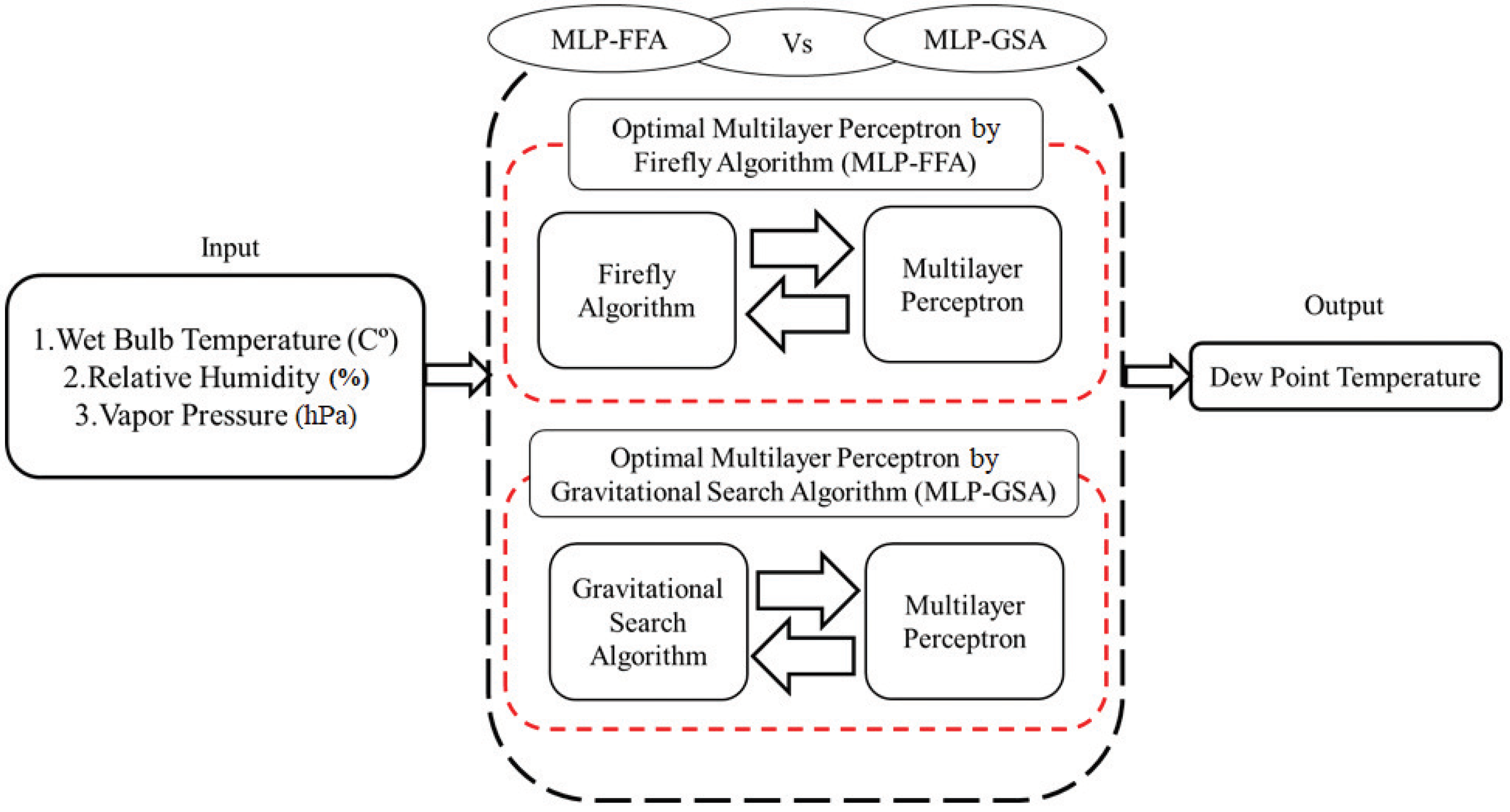
2.1. Multilayer Perceptron Neural Network

In the current study, a multilayer perceptron (MLP) neural network was employed since it is one of the predominant versions of neural network models used globally [39]. MLP has been widely used in hydrological modeling owing to its simplicity, robustness, and the advantage from error back propagation [40,41,42]. The network structure includes three layers of nodes (neurons), namely, the input, hidden, and output layer, as presented in Figure 1. The active input layer receives the data supplied by the user and passes to the hidden layer, which is sandwiched across the input and output layers. Weights are specified for all the connections. Biases and activation functions are proposed for each of the hidden and output nodes. The MLP network learns from a predefined set of an input–output pair in two cycles—propagate and adapt cycle. The back-propagation algorithm is generally used to train the MLP network, which involves a learning rate parameter that aids in adapting all the weights and biases to the optimal values. The weights are adjusted in a way that minimizes the error. These steps are repeated until the error for the entire set is acceptably low with the provision of sufficient training [43]. In the present study, the sigmoid and linear activation functions were considered during network calibration in the hidden and output layers, respectively. The relatively fast Levenberg–Marquardt (LM) back propagation learning algorithm with adaptive momentum was used for escalating the convergence speed of the MLP. This architecture is also well-known for arriving at the best combination of initial weights and biases which minimizes the cost function (mean square error (MSE) statistic) and lead to a global optimal solution of the problem. More theoretical details and description with regard to the multilayer perceptron model can be found in previous research works [44,45,46].

2.2. Hybridized MLP–FFA Models

Among several nature-inspired optimisation algorithms, the firefly algorithm (FFA) proposed recently by the authors of [36] provides a great flexibility to hybridize with MLP neural network to make an efficient implementation for any kind of time-series analysis tasks. The firefly algorithm is a nature-inspired, swarm intelligence technique derived from the flashing and attraction behavior of fireflies. Its metaheuristic property allows users to search for optimal parameters of the multilayer perceptron model. Every individual firefly is distinguished by its light intensity and the degree of attractiveness. In this context, FFA is incorporated with MLP to update the weights, bias, and number of hidden neurons of the neural network. In every iteration, the deviation of modeled output from that of the expected is found in terms of ‘error criteria/cost function’—for example, in this case, mean square error (MSE), to upgrade the model parameters in successive steps. If the stopping criterion (i.e., the MSE ≅ 0) is not met, the variations of light intensity and change in the attractiveness of all the flies are updated again and ranked. The MLP training process continues until the stopping criterion is met. Each splendid firefly can draw the attention of its neighborhood fireflies, regardless of their sex, and the attractiveness is relative to its brightness, which makes the exploration of optimal search space progressively productive [47]. The essential errand in the design of the MLP–FFA model is defining the objective function and formulating the variations of light intensity and attractiveness of fireflies. The intensity of light emitted from fireflies diminishes with the distance from its source and due to absorption by the media. Mathematically, the light intensity ‘I’ varies exponentially with the distance r and light absorption parameter γ , which is represented as follows [36,47,48]:
I = I o · e γ r 2 ,
where I o is the initial light intensity at the source (i.e., at the distance r = 0) and γ is the light absorption coefficient. Since it is assumed that the attractiveness of firefly is directly proportional to the light intensity I, the firefly’s light attractive coefficient β is defined in the similar way as the light intensity coefficient I. That is:
β = β o · e γ r 2 ,
where β o is the initial light attractiveness at r = 0. The Cartesian distance between any two fireflies i and j at x i and x j is given by:
r i j = x i + x j 2 = k = 1 d ( x i , k x j , k ) 2 ,
where d is the number of dimensions and k represents component in spatial co-ordinate. The next movement of a firefly i towards another brightest firefly j is given by:
x i i + 1 = x i + Δ x i ,
Δ x i = β o · e γ r 2 ( x j x i ) + α ϵ i ,
where the 1st term in Equation (5) emerges due to the attraction effect and the 2nd term represents the randomization parameter, with α as a scaling co-efficient whose values are registered between 0 and 1, while ϵ i is a vector of random variables derived from different distributions, such as the uniform distribution, Gaussian distribution, and Lévy flight. For details related to the mathematics of FFA, one can refer to the following literature: References [36,47,48]. Figure 2 demonstrates a schematic perspective of the process of obtaining the optimal hidden layer weights of MLP with the use of the firefly algorithm for the estimation of daily dew point temperature. The hybrid MLP–FFA algorithm has been successfully implemented to model pan evaporation [41], water quality parameters—the BOD and DO of Langat river [49], lake water level prediction [50], and wind speed prediction [51].

2.3. Hybridized MLP–GSA Model

The gravitational dearch algorithm (GSA) was introduced by Reference [35]. GSA is based on the concept of the population search of the Newtonian gravity principle. In the present study, GSA is used for arriving at optimal weights and biases of the MLP network which satisfy the minimum error criteria. Initially, to evaluate an agent’s fitness, preferably any error criteria of the fitness function, such as MSE, should be defined along with a strategy to encode the optimal weights and biases of the MLP network [52]. The positions of ‘agents’, also referred to as ‘objects’, are the solutions in the GSA population and the fitness function is determined by the gravitational and inertial masses of the agents. Due to gravitational force, all the lighter objects are attracted towards the object with heavier mass in proportion to their distances, thus representing a global movement (exploration step) of the objects. The slow movement of heavier objects (good solutions) guarantees the exploitation step of the GSA algorithm. The optimization process of GSA starts with the positioning of agents randomly with random velocity values and initialization of the gravitational constant. Consequently, the fitness of each agent according to the defined objective function is evaluated, and the gravitational constant, G ( t ) , is updated. At a specific time t, the force acting on object i due to the movement of object j is defined by:
F i j d ( t ) = G ( t ) M p i ( t ) × M a j ( t ) R i j ( t ) + ε x j d ( t ) x i d ( t ) ,
where M a j is the active gravitational mass related to agent j and M p i is the passive gravitational mass related to agent i . The gravitational constant G ( t ) and the Euclidian distance R i j ( t ) between two agents i and j are calculated as follows:
G ( t ) = G o · e x p α × i t e r m a x i t e r ,
R i j ( t ) = X i ( t ) , X j ( t ) 2 ,
where α is the descending coefficient, G o is the initial gravitational constant, i t e r is the current iteration, and m a x i t e r is the maximum number of iterations. In a d dimensional problem space, the total force that acts on agent i is given by:
F i d ( t ) = j = 1 , j 1 N r a n d j F i j d ( t ) ,
where r a n d j is a random number in the interval [0, 1]. Based on the law of motion, the acceleration of all agents at time t , and in d t h direction is calculated as follows:
a i d ( t ) = F i d ( t ) M i i ( t ) ,
where M i i is the inertial mass of i t h agent. Furthermore, the searching strategy of an agent is dependent on the velocity and position of agents which are calculated as follows:
v i d ( t + 1 ) = r a n d i × v i d ( t ) + a i d ( t ) ,
x i d ( t + 1 ) = x i d ( t ) + v i d ( t + 1 ) .
The updating process is repeated as long as the stopping criterion is not satisfied. When a certain stopping criterion is met, or soon after the maximum number of iterations are reached, the GSA algorithm ceases. The superiority of GSA is due to two steps: Exploration (potential to navigate in the space) and exploitation (potential to search optima around the best solution). For additional details related to GSA, one may refer to Xing and Gao (2014) [53] and Jadidi et al. (2013) [54]. The schematic structure of the MLP–GSA is shown in Figure 2.

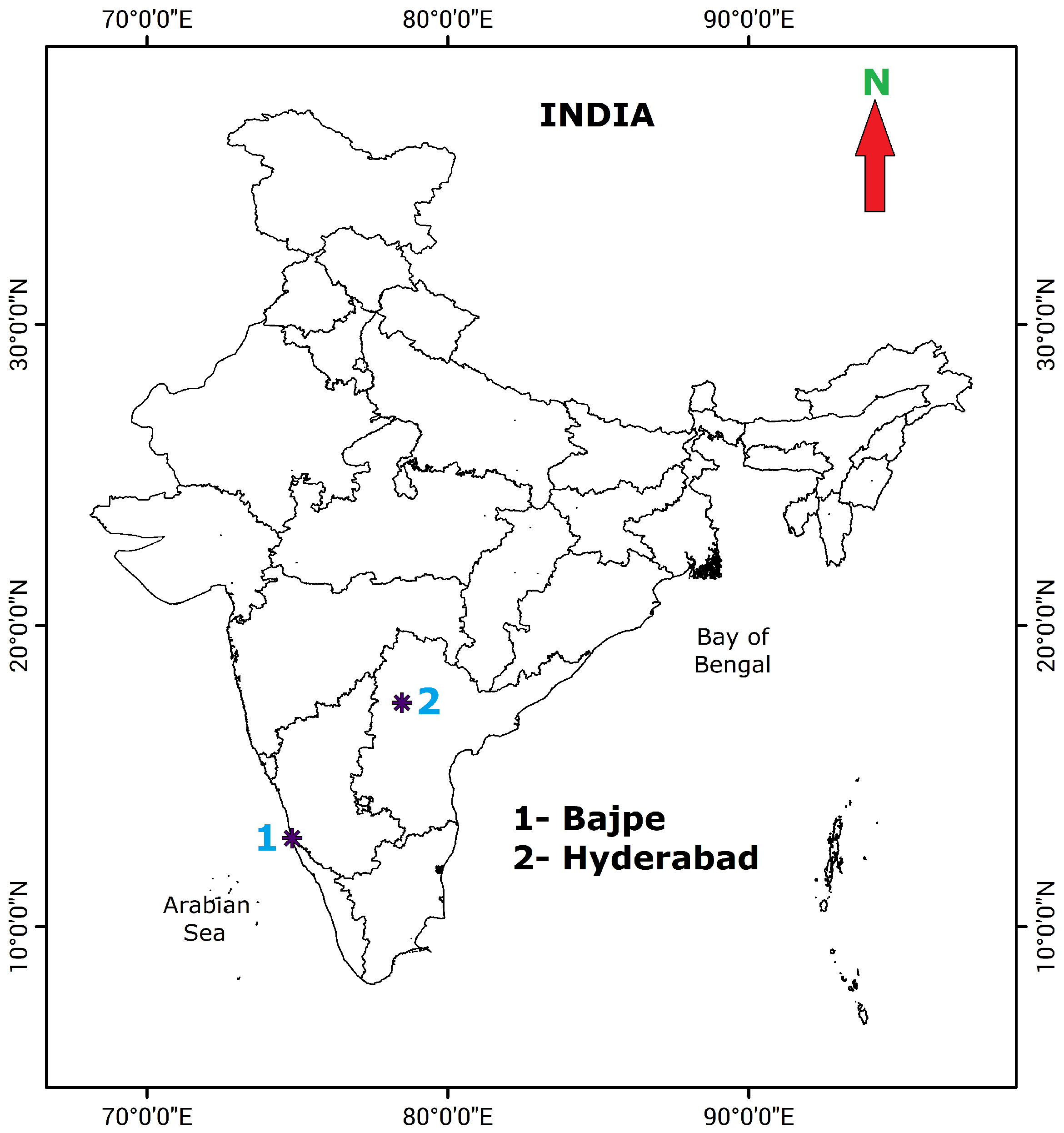
3. Study Area and Data Description

The two regions of interest investigated in the present research belong to diverse climatic zones, and the purpose was to estimate the DPT using two hybrid MLP neural network models, namely, the MLP–FFA and MLP–GSA models. The performance of these was compared with that of the standalone MLP, SVM, and ELM models. The weather information pertaining to the Bajpe and Hyderabad locations of the time-period 2006–2009 procured from the Indian Meteorological Department (IMD), India were used for DPT modeling. Most of the Western ghat region around the Bajpe weather station ( 17.44 ° N, 78.47 ° E) witnesses a humid tropical climate and the deccan plateau in the vicinity of Hyderabad weather station ( 12.94 ° N, 74.82 ° E) experiences a semi-arid or steppe climate. Bajpe experiences a shorter dry season and falls under the category of a tropical monsoon climate (Am) as per the Köppen–Geiger climate classification system [55]. The average annual temperature and rainfall in and around Bajpe is 27.0 ° C and 3700 mm, respectively, with high humidity levels above 75% on an average. The climate of Hyderabad is hot semi-arid and is classified as BSh in the Köppen–Geiger system. This region receives medium annual rainfall (ranging from 300 to 600 mm) with humidity levels in 30–55% range. Figure 3 presents the location map of the Bajpe and Hyderabad weather stations.
This study sourced daily weather data from the Indian Meteorological Department that include four attributes, namely, the vapor pressure, wet bulb temperature, relative humidity, and DPT of Bajpe and Hyderabad locations measured at two times of a day on the 3rd hour and 12th hour UTC. The Bajpe weather data comprised 669 daily observations of the time period—January 2005 to October 2006. The training dataset included daily data of the 16-month time period starting from January 2005 to April 2006 and the residual data of the time period—May 2006 to October 2006—was hoarded for model testing. In the same way, the Hyderabad weather data included 1047 daily observations from the time period of January 2007 to December 2009. The model calibration embraced weather data of a 26-month time period from January 2007 to February 2009, and the residual data of a 10-month time period from March 2009 to December 2009 were hoarded for testing of the developed models. The most influential weather parameters that supplement as inputs for DPT estimation were found by cross-correlation analysis. The vapor pressure, wet bulb temperature, and relative humidity were found to have good correlation with DPT (refer to Table 1) and were hence considered as input attributes. Table 2 presents the statistical parameters such as mean, maximum (Max), minimum (Min), standard deviation (S.Dev.), skewness (Skew), and variance (Var.) of weather parameters employed in the study.

4. Model Development and Performance Analysis

The input/output (I/O) structure formulated for the development of MLP–FFA, MLP–GSA, and the standalone AI models were based on the correlated weather information with the target variable—DPT (Table 1). The DPT models of the 3rd hour and 12th hour UTC were calibrated individually using the I/O structure as mentioned below.
D e w P o i n t T e m p e r a t u r e ( D P T ) f [ W B T + R H + V P ]
MLP training refers to a search process for identification of an optimized set of weight and bias values, which can minimize the mean squared error (MSE) across the estimated and real data in the output layer. As already mentioned, a standalone MLP network was trained using an LM back-propagation algorithm. A structured trial and error method was used to find the optimal number of hidden layer neurons, values of the learning rate, and momentum terms in accordance to the minimum MSE criteria. The FFA and GSA parameters used while training the hybrid MLP models are mentioned in Table 3. The learning rate (which controls weight and bias change in each iteration) and the number of hidden neurons of MLP were optimized using the FFA and GSA algorithms. The proposed hybrid ML models were developed using Matlab software.
Performance evaluation: The statistical evaluation measures are endowed with confidence that could be relayed on any model estimates. In the present case, the error and efficiency measures such as RMSE, MAE, and NSE were employed to assess the model performance.
Root mean square error (RMSE):
R M S E = i = 1 n ( x i y i ) 2 n
Mean absolute error (MAE):
M A E = i = 1 n y i x i n
Nash Sutcliffe efficiency (NSE):
N S E = 1 i = 1 n ( y i x i ) 2 i = 1 n ( x i x ¯ ) 2
where x i —the actual observation; y i —the predicted value; x ¯ —mean observation; n—number of examined dataset.

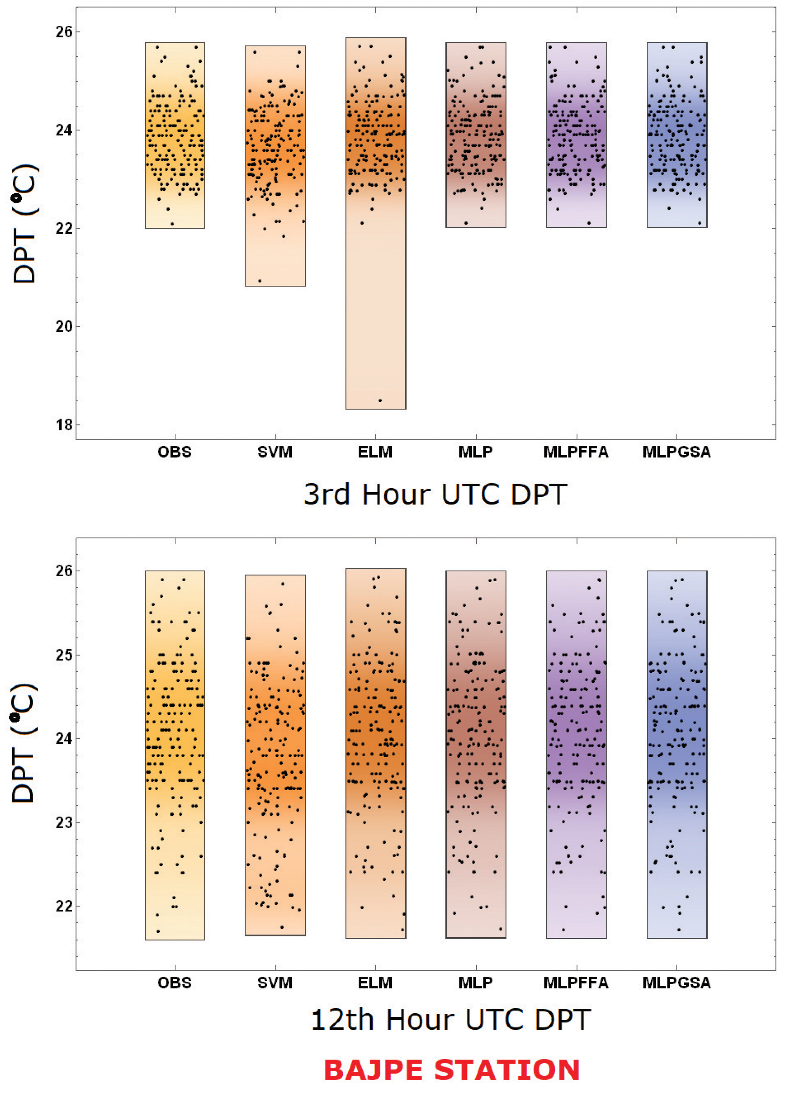
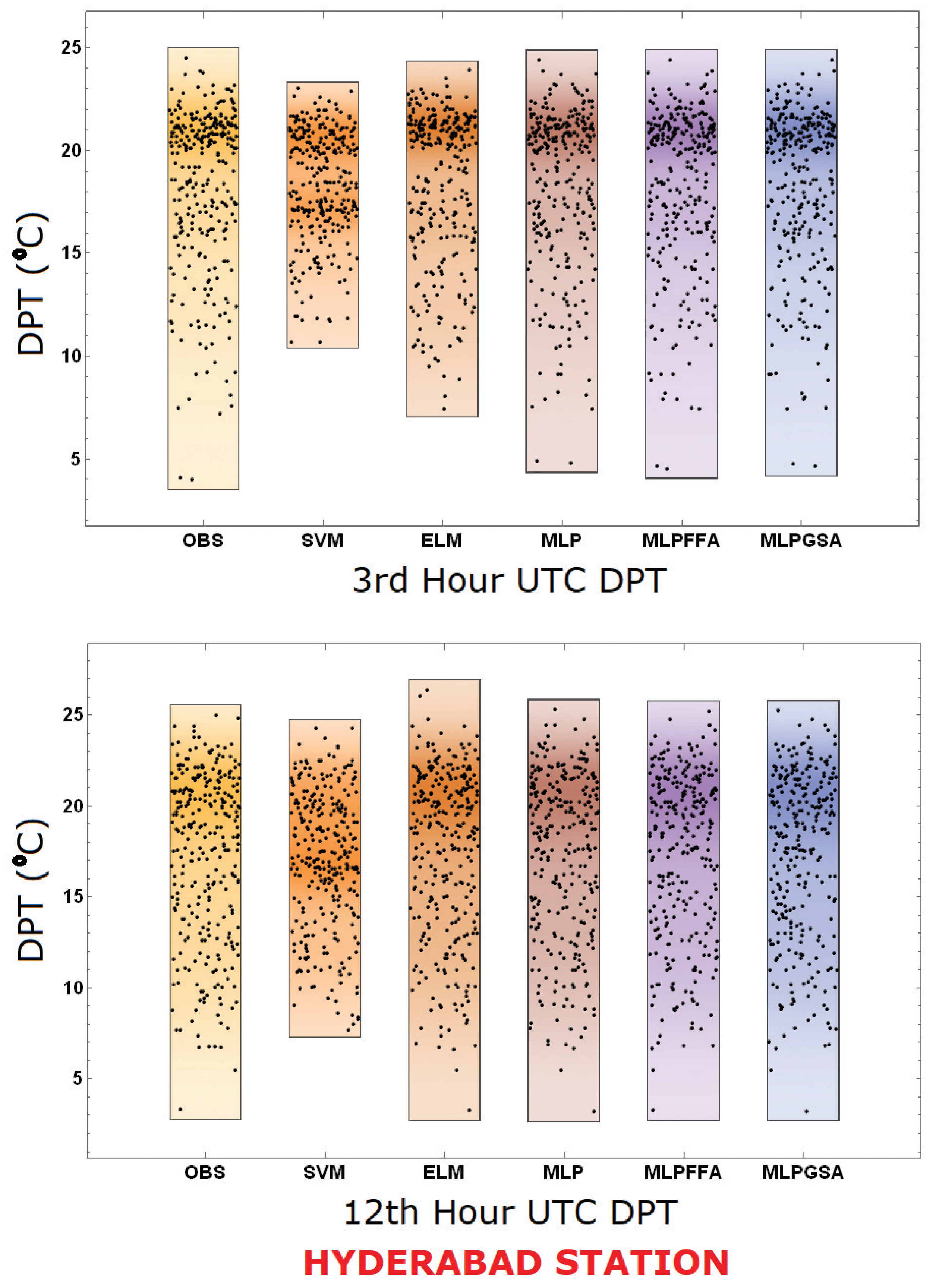
5. Results and Discussion

Without any doubt, there exist several soft computing models that have shown excellent performance in modeling dew point temperature [24,28]. However, researchers have been extremely zealous to navigate through new methodologies for the sake of attaining more reliable and robust models for solving any kind of complex nonlinear problems. The current research demonstrated the hybridization of the classical artificial intelligence model with nature-inspired optimization algorithms for impersonating the actual physic concept—DPT. The performance of hybrid models (i.e., MLP–FFA and MLP–GSA) in estimating daily DPT were evaluated against SVM and ELM model results reported in Deka et al. (2018) [26], since the models developed in this study used the same data and model (input–output) structure of the earlier research by Deka et al. (2018) [26]. Table 4 and Table 5 present the performance of hybrid MLP networks (MLP–FFA and MLP–GSA) and other models (MLP, SVM, and ELM), evaluated in terms of various performance statistics along with relevant model parameters or network configurations. The input variables (wet bulb temperature (WBT), relative humidity (RH), and vapor pressure (VP)) derived from the cross-correlation analyses in conjunction with the dependent variable (DPT) were appropriate for model development and therefore resulted in good efficiency measures.
With reference to Bajpe weather station, the MLP–FFA hybrid model is consistently the superior one when compared to others in terms of all performance statistics for the estimation of both the 3rd and 12th hour UTC DPT (see Table 4). In parallel, the efficiencies of MLP–GSA revealed similar skills in the estimation process. It can be observed that the absolute error measurements indicated the superiority of the proposed hybrid models over MLP, SVM, and ELM estimates. In quantitative terms, for instance, the MLP–FFA model reported a remarkable enhancement of RMSE/MAE by (33/31%), (91/73%), and (92/95%) over the MLP, SVR, and ELM models, respectively; and likewise, the MLP–GSA model estimates reported a percentage enhancement by (19/18%), (89/67%), and (91/93%) over the MLP, SVM, and ELM models, respectively (in the case of the 3rd hour DPT modeling). The hybridization of nature-inspired algorithms with MLP proved to yield powerful predictive models and can contribute to modeling any kind of environmental processes.
With reference to Hyderabad weather station, the hybrid MLP–FFA and MLP–GSA networks again validated superior performance with the same statistical metrics run for the previous one (see Table 5). In this case, what can be noticed remarkably is the NSE values which are very close to unity, indicating a superior performance by the models. The comparative analysis of model performance measures reveals that the DPT estimates of standard MLP and its hybrid structures (MLP–FFA and MLP–GSA) have low error estimates (RMSE and MSE) in contrast to the SVM and ELM models. The performance of the MLP–FFA networks was relatively superior to the MLP–GSA models in terms of computational speed and accuracy. The speed of convergence of FFA is very high in probability of finding the global optimized solutions because of Gaussian or Lévy flight searches, and sometimes, the FFA is considered as a generalization to three different approaches, namely, particle swarm optimization (PSO), simulated annealing (SA), and differential evolution (DE) [48]. It is evident that= the integration of GSA with MLP also provides good estimates of DPT, and the gravitational constant and acceleration of particles are the parameters that are crucial in regulating the exploratory capabilities of the GSA algorithm [56].
An excellent way of graphical presentation was considered for the prediction skill illustration through Taylor diagrams (see Figure 4 and Figure 5), for both the 3rd and 12th hour UTC DPT models. The Taylor diagram provides a concise statistical summary of modeled data in terms of its standard deviation, root mean square difference and the correlation with actual data [57]. It shows how well the predictive models match the actual records of DPT of the testing phase with regard to both investigated climate zones. The relative merits of models developed can be assessed from high correlation and low RMS errors represented by points nearest to the reference point (i.e., the actual data). The result statistics of the MLP–FFA and MLP–GSA models were closer to the observation point, reaffirming the better accuracy of the hybridized models over its comparison counterparts. On comparing the point–density plots, presented in Figure 6 and Figure 7, no significant differences were evident among the pair of observed vs. (MLP–FFA and MLP–GSA) model estimates with respect to the extreme (minimum and maximum) values and any outliers. It is also evident that the spreads of observed vs. (SVM and ELM) modeled DPTs fluctuate and were dissimilar to each other, assuring variations in the overall pattern of the estimated time-series data.
Taking into account the disadvantages of the back-propagation (BP) algorithm as discussed in the earlier part of the manuscript, the novel methods of network adaptation were tested via the FFA and GSA algorithms, by implementing the phase of nonrandom initialization of weight vector ‘w’. It is nothing unexpected that the MLP network integrated with FFA or GSA for weights adjustment gave altogether better results than the standard MLP. Moreover, in addition to lower RMSE and MAE, another advantage of hybridizing MLP with FFA or GSA is the consistency of estimates. The NSEs of the MLP–FFA and MLP–GSA networks are remarkably higher than those of the SVM and ELM models. The acceptable level of accuracy attained using the proposed methodology evidenced the potential of the hybrid intelligent models for DPT estimation where it is highly essential for practical implementation, and especially in the case of designing an online estimation system for monitoring the DPT fluctuation and using that accurate information for water engineering management and its related applications.
It is worth reporting here, since the main focus of the current research was on the development and application of hybrid MLP models for dew point temperature estimation, the uncertainty estimation and analysis using statistical methods would be one of the possible future focuses of research. As a matter of fact, the uncertainties are incorporated in different forms, such as data uncertainty, modeling uncertainty, and input variability uncertainty. Hence, investigating those types of uncertainties is highly essential for modeling predictability evaluation.

6. Conclusions

Dew point temperature estimation is of great interest to agro–climatologists for several studies that need continuous DPT data. The missing DPT data records could be in-filled using several estimation techniques. In recent times, time-series based machine learning algorithms have been advantageous over conventional physics-based approaches in terms of solving complex regression problems with less computational cost. This study was intended to explore new hybrid intelligent predictive models to estimate DPTs of humid and semi-arid regions of India. The hybrid MLP–FFA and MLP–GSA networks were trained to estimate the daily DPTs using correlated weather variables, including WBT, RH, and VP, as inputs. MLP–FFA obtained the best results with significantly faster convergence ability. The three evaluation indices gave definitely no reason to discard the superiority of MLP and its hybrid structures over the SVM and ELM models. The efficiency of the MLP network is dependent on the optimal tuning for the input parameters in addition to architecture type and training algorithm employed. The nature-inspired optimization algorithms certainly augment the predictability of the classical MLP model. The performance of both the MLP–FFA and MLP–GSA networks exhibited an acceptable level of accuracy and enhancement for both inspected climactic zones. However, MLP–FFA emerged as the most optimal technique compared to others in terms of the minimum error criteria.

Author Contributions

Conceptualization, S.R.N.; Data analysis, S.R.N.; Formal analysis, S.M.B.; Funding acquisition, N.A.-A.; Investigation, S.M.B.; Methodology, M.A.G.; Project administration, S.M.B.; Software, S.R.N. and M.A.G.; Supervision, P.C.D.; Validation, Z.M.Y.; Visualization, Z.M.Y.; Writing—original draft, S.R.N.; Writing—review and editing, Z.M.Y., P.C.D., and N.A.-A.

Funding

This research received no external funding.

Acknowledgments

The scholars of the present work would like to reveal their gratitude and appreciation to the data provider, the Indian Meteorological Department, Ministry of Earth Sciences, Govt. of India.

Conflicts of Interest

The authors declare no conflict of interest.

References

  1. Wood, L.A. The use of dew-point temperature in humidity calculations. J. Res. Notional Bur. Stand. 1970, 74, 117–122. [Google Scholar] [CrossRef]
  2. Ben-Asher, J.; Alpert, P.; Ben-Zvi, A. Dew is a major factor affecting vegetation water use efficiency rather than a source of water in the eastern Mediterranean area. Water Resour. Res. 2010, 46, W10532. [Google Scholar] [CrossRef]
  3. Ahrens, C.D. Meteorology Today; Chapter Condensation: Dew, Fog, and Clouds; Thomson Higher Education: Belmont, CA, USA, 2007; pp. 106–137. [Google Scholar]
  4. Changnon, D.; Sandstrom, M.; Schaffer, C. Relating changes in agricultural practices to increasing Dew points in extreme Chicago heat waves. Clim. Res. 2003, 24, 243–254. [Google Scholar] [CrossRef]
  5. McHugh, T.A.; Morrissey, E.M.; Reed, S.C.; Hungate, B.A.; Schwartz, E. Water from air: An overlooked source of moisture in arid and semiarid regions. Sci. Rep. 2015, 5, 13767. [Google Scholar] [CrossRef] [PubMed]
  6. Agam, N.; Berliner, P. Dew formation and water vapor adsorption in semi-arid environments—A review. J. Arid Environ. 2006, 65, 572–590. [Google Scholar]
  7. Eccel, E. Estimating air humidity from temperature and precipitation measures for modelling applications. Meteorol. Appl. 2012, 19, 118–128. [Google Scholar] [CrossRef]
  8. Ebrahimpour, M.; Ghahreman, N.; Orang, M. Assessment of climate change impacts on reference evapotranspiration and simulation of daily weather data using SIMETAW. J. Irrig. Drain. Eng. 2014, 140, 04013012. [Google Scholar] [CrossRef]
  9. Mahmood, R.; Hubbard, K.G. Assessing bias in evapotranspiration and soil moisture estimates due to the use of modeled solar radiation and dew point temperature data. Agric. For. Meteorol. 2005, 130, 71–84. [Google Scholar] [CrossRef]
  10. McMahon, T.; Peel, M.; Lowe, L.; Srikanthan, R.; McVicar, T. Estimating actual, potential, reference crop and pan evaporation using standard meteorological data: A pragmatic synthesis. Hydrol. Earth Syst. Sci. 2013, 17, 1331–1363. [Google Scholar] [CrossRef]
  11. Roberts, J.S. Encyclopedia of Agricultural, Food and Biological Engineering; Chapter Dew Point Temperature; CRC Press: Boca Raton, FL, USA, 2003; pp. 186–191. [Google Scholar]
  12. Lawrence, M.G. The relationship between relative humidity and the Dewpoint temperature in moist air: A simple conversion and applications. Bull. Am. Meteorol. Soc. 2005, 86, 225–233. [Google Scholar]
  13. Pokhrel, P.; Wang, Q.; Robertson, D.E. The value of model averaging and dynamical climate model predictions for improving statistical seasonal streamflow forecasts over Australia. Water Resour. Res. 2013, 49, 6671–6687. [Google Scholar] [CrossRef] [Green Version]
  14. Liu, Z.; Zhou, P.; Chen, X.; Guan, Y. A multivariate conditional model for streamflow prediction and spatial precipitation refinement. J. Geophys. Res. Atmos. 2015, 120. [Google Scholar] [CrossRef]
  15. Liu, Z.; Cheng, L.; Hao, Z.; Li, J.; Thorstensen, A.; Gao, H. A framework for exploring joint effects of conditional factors on compound floods. Water Resour. Res. 2018, 54, 2681–2696. [Google Scholar] [CrossRef]
  16. Khedun, C.P.; Mishra, A.K.; Singh, V.P.; Giardino, J.R. A copula-based precipitation forecasting model: Investigating the interdecadal modulation of ENSO’s impacts on monthly precipitation. Water Resour. Res. 2014, 50, 580–600. [Google Scholar] [CrossRef]
  17. Tao, H.; Diop, L.; Bodian, A.; Djaman, K.; Ndiaye, P.M.; Yaseen, Z.M. Reference evapotranspiration prediction using hybridized fuzzy model with firefly algorithm: Regional case study in Burkina Faso. Agric. Water Manag. 2018, 208, 140–151. [Google Scholar] [CrossRef]
  18. Shank, D.B.; McClendon, R.W.; Paz, J.; Hoogenboom, G. Ensemble Artificial Neural Networks for prediction of Dew point temperature. Appl. Artif. Intell. 2008, 22, 523–542. [Google Scholar] [CrossRef]
  19. Zounemat-Kermani, M. Hourly predictive Levenberg–Marquardt ANN and multi linear regression models for predicting of Dew point temperature. Meteorol. Atmos. Phys. 2012, 117, 181–192. [Google Scholar] [CrossRef]
  20. Nadig, K.; Potter, W.; Hoogenboom, G.; McClendon, R. Comparison of individual and combined ANN models for prediction of air and Dew point temperature. Appl. Intell. 2013, 39, 354–366. [Google Scholar] [CrossRef]
  21. Kisi, O.; Kim, S.; Shiri, J. Estimation of Dew point temperature using Neuro-fuzzy and Neural network techniques. Theor. Appl. Climatol. 2013, 114, 365–373. [Google Scholar] [CrossRef]
  22. Shiri, J.; Kim, S.; Kisi, O. Estimation of daily Dew point temperature using Genetic Programming and Neural Networks approaches. Hydrol. Res. 2014, 45, 165–181. [Google Scholar] [CrossRef]
  23. Kim, S.; Singh, V.P.; Lee, C.J.; Seo, Y. Modeling the physical dynamics of daily Dew point temperature using soft computing techniques. KSCE J. Civ. Eng. 2015, 19, 1930–1940. [Google Scholar] [CrossRef]
  24. Mohammadi, K.; Shamshirband, S.; Motamedi, S.; Petković, D.; Hashim, R.; Gocic, M. Extreme learning machine based prediction of daily Dew point temperature. Comput. Electron. Agric. 2015, 117, 214–225. [Google Scholar] [CrossRef]
  25. Mohammadi, K.; Shamshirband, S.; Petković, D.; Yee, L.; Mansor, Z. Using ANFIS for selection of more relevant parameters to predict Dew point temperature. Appl. Therm. Eng. 2016, 96, 311–319. [Google Scholar] [CrossRef]
  26. Deka, P.C.; Patil, A.P.; Yeswanth Kumar, P.; Naganna, S.R. Estimation of dew point temperature using SVM and ELM for humid and semi-arid regions of India. ISH J. Hydraul. Eng. 2018, 24, 190–197. [Google Scholar] [CrossRef]
  27. Attar, N.F.; Khalili, K.; Behmanesh, J.; Khanmohammadi, N. On the reliability of soft computing methods in the estimation of dew point temperature: The case of arid regions of Iran. Comput. Electron. Agric. 2018, 153, 334–346. [Google Scholar] [CrossRef]
  28. Baghban, A.; Bahadori, M.; Rozyn, J.; Lee, M.; Abbas, A.; Bahadori, A.; Rahimali, A. Estimation of air Dew point temperature using computational intelligence schemes. Appl. Therm. Eng. 2016, 93, 1043–1052. [Google Scholar] [CrossRef]
  29. Al-Shammari, E.T.; Mohammadi, K.; Keivani, A.; Ab Hamid, S.H.; Akib, S.; Shamshirband, S.; Petković, D. Prediction of daily dewpoint temperature using a model combining the support vector machine with firefly algorithm. J. Irrig. Drain. Eng. 2016, 142, 04016013. [Google Scholar] [CrossRef]
  30. Amirmojahedi, M.; Mohammadi, K.; Shamshirband, S.; Danesh, A.S.; Mostafaeipour, A.; Kamsin, A. A hybrid computational intelligence method for predicting dew point temperature. Environ. Earth Sci. 2016, 75, 415. [Google Scholar] [CrossRef]
  31. Ludermir, T.B.; Yamazaki, A.; Zanchettin, C. An optimization methodology for neural network weights and architectures. IEEE Trans. Neural Networks 2006, 17, 1452–1459. [Google Scholar] [CrossRef]
  32. Lawrence, S.; Giles, C.L.; Tsoi, A.C. What Size Neural Network Gives Optimal Generalization? Convergence Properties of Backpropagation; Technical Report CS-TR-3617; University of Maryland: College Park, MD, USA, 1996. [Google Scholar]
  33. Lawrence, S.; Giles, C.L. Overfitting and neural networks: Conjugate gradient and backpropagation. In Proceedings of the IEEE-INNS-ENNS International Joint Conference on Neural Networks, Como, Italy, 27 July 2000; Volume 1, pp. 114–119. [Google Scholar]
  34. Nayak, J.; Naik, B.; Behera, H. A novel nature inspired firefly algorithm with higher order neural network: Performance analysis. Eng. Sci. Technol. Int. J. 2016, 19, 197–211. [Google Scholar] [CrossRef] [Green Version]
  35. Rashedi, E.; Nezamabadi-pour, H.; Saryazdi, S. GSA: A Gravitational Search Algorithm. Inf. Sci. 2009, 179, 2232–2248. [Google Scholar] [CrossRef]
  36. Yang, X.S. Firefly algorithm, stochastic test functions and design optimisation. Int. J. Bio-Inspired Comput. 2010, 2, 78–84. [Google Scholar] [CrossRef]
  37. Siddiquea, N.; Adelib, H. Applications of gravitational search algorithm in engineering. J. Civ. Eng. Manag. 2016, 22, 981–990. [Google Scholar] [CrossRef]
  38. Yang, X.S.; He, X. Firefly algorithm: Recent advances and applications. Int. J. Swarm Intell. 2013, 1, 36–50. [Google Scholar] [CrossRef]
  39. Gardner, M.W.; Dorling, S. Artificial Neural Networks (the Multilayer Perceptron)–a review of applications in the atmospheric sciences. Atmos. Environ. 1998, 32, 2627–2636. [Google Scholar] [CrossRef]
  40. Fabbian, D.; de Dear, R.; Lellyett, S. Application of artificial neural network forecasts to predict fog at Canberra International Airport. Weather Forecast. 2007, 22, 372–381. [Google Scholar] [CrossRef]
  41. Ghorbani, M.; Deo, R.C.; Yaseen, Z.M.; Kashani, M.H.; Mohammadi, B. Pan evaporation prediction using a hybrid multilayer perceptron-firefly algorithm (MLP-FFA) model: Case study in North Iran. Theor. Appl. Climatol. 2018, 133, 1119–1131. [Google Scholar] [CrossRef]
  42. Ghorbani, M.A.; Zadeh, H.A.; Isazadeh, M.; Terzi, O. A comparative study of artificial neural network (MLP, RBF) and support vector machine models for river flow prediction. Environ. Earth Sci. 2016, 75, 476. [Google Scholar] [CrossRef]
  43. Rumelhart, D.E.; McClelland, J.L. Parallel Distributed Processing; MIT Press: Cambridge, MA, USA, 1987; Volume 1. [Google Scholar]
  44. Lek, S.; Park, Y. Artificial Neural Networks. In Encyclopedia of Ecology; Academic Press: Oxford, UK, 2008; pp. 237–245. [Google Scholar]
  45. Haykin, S.S. Neural Networks and Learning Machines, 3rd ed.; Prentice-Hall: Upper Saddle River, NJ, USA, 2009; p. 906. [Google Scholar]
  46. Park, Y.S.; Lek, S. Artificial Neural Networks: Multilayer Perceptron for Ecological Modeling. In Ecological Model Types; Developments in Environmental Modelling; Elsevier: Amsterdam, The Netherlands, 2016; Volume 28, pp. 123–140. [Google Scholar]
  47. Zhang, L.; Liu, L.; Yang, X.S.; Dai, Y. A Novel Hybrid Firefly Algorithm for Global Optimization. PLoS ONE 2016, 11, 1–17. [Google Scholar] [CrossRef]
  48. Iztok, F.; Iztok, F.J.; Xin-She, Y.; Janez, B. A comprehensive review of Firefly algorithms. Swarm Evol. Comput. 2013, 13, 34–46. [Google Scholar]
  49. Raheli, B.; Aalami, M.T.; El-Shafie, A.; Ghorbani, M.A.; Deo, R.C. Uncertainty assessment of the multilayer perceptron (MLP) neural network model with implementation of the novel hybrid MLP-FFA method for prediction of biochemical oxygen demand and dissolved oxygen: A case study of Langat River. Environ. Earth Sci. 2017, 76, 503. [Google Scholar] [CrossRef]
  50. Ghorbani, M.A.; Deo, R.C.; Karimi, V.; Yaseen, Z.M.; Terzi, O. Implementation of a hybrid MLP-FFA model for water level prediction of Lake Egirdir, Turkey. Stoch. Environ. Res. Risk Assess. 2017, 32, 1683–1697. [Google Scholar] [CrossRef]
  51. Deo, R.C.; Ghorbani, M.A.; Samadianfard, S.; Maraseni, T.; Bilgili, M.; Biazar, M. Multi-layer perceptron hybrid model integrated with the Firefly optimizer algorithm for windspeed prediction of target site using a limited set of neighboring reference station data. Renew. Energy 2018, 116, 309–323. [Google Scholar] [CrossRef]
  52. Mirjalili, S.; Hashim, S.Z.M.; Sardroudi, H.M. Training Feedforward Neural Networks using hybrid particle swarm optimization and Gravitational Search Algorithm. Appl. Math. Comput. 2012, 218, 11125–11137. [Google Scholar] [CrossRef]
  53. Xing, B.; Gao, W.J. Gravitational Search Algorithm. In Innovative Computational Intelligence: A Rough Guide to 134 Clever Algorithms; Springer International Publishing: Berlin, Germany, 2014; pp. 355–364. [Google Scholar]
  54. Jadidi, Z.; Muthukkumarasamy, V.; Sithirasenan, E.; Sheikhan, M. Flow-Based Anomaly Detection Using Neural Network Optimized with GSA Algorithm. In Proceedings of the 2013 IEEE 33rd International Conference on Distributed Computing Systems Workshops, Philadelphia, PA, USA, 8–11 July 2013; pp. 76–81. [Google Scholar]
  55. Peel, M.C.; Finlayson, B.L.; McMahon, T.A. Updated world map of the Köppen-Geiger climate classification. Hydrol. Earth Syst. Sci. 2007, 11, 1633–1644. [Google Scholar] [CrossRef]
  56. De Moura Oliveira, P.B.; Oliveira, J.; Cunha, J.B. Trends in Gravitational Search Algorithm. In 14th International Conference on Distributed Computing and Artificial Intelligence; Omatu, S., Rodríguez, S., Villarrubia, G., Faria, P., Sitek, P., Prieto, J., Eds.; Springer International Publishing: Berlin, Germany, 2018; pp. 270–277. [Google Scholar]
  57. Taylor, K.E. Summarizing multiple aspects of model performance in a single diagram. J. Geophys. Res. Atmos. 2001, 106, 7183–7192. [Google Scholar] [CrossRef] [Green Version]
Figure 1. Artificial neural network (MLP) structure.
Water 11 00742 g001
Figure 2. Schematic structure of the hybrid multilayer perceptron–firefly algorithm (MLP–FFA) and MLP–gravitational search algorithm (MLP–GSA) methods applied for dew point temperature estimation.
Water 11 00742 g002
Figure 3. The coordinate of the inspected meteorological stations.
Water 11 00742 g003
Figure 4. Taylor diagram for performance evaluation of the models with respect to Bajpe station.
Water 11 00742 g004
Figure 5. Taylor diagram for performance evaluation of the models with respect to Hyderabad station.
Water 11 00742 g005
Figure 6. Point density plots of observed vs. estimated DPTs with respect to Bajpe station.
Water 11 00742 g006
Figure 7. Point density plots of observed vs. estimated DPTs with respect to Hyderabad station.
Water 11 00742 g007
Table 1. Correlation coefficient statistic of DPT with other model input attributes.
Correlation
Co-Efficient
Bajpe StationHyderabad Station
3rd Hour UTC12th Hour UTC3rd Hour UTC12th Hour UTC
DPT ( ° C)DPT ( ° C)DPT ( ° C)DPT ( ° C)
WBT ( ° C)0.970.90.90.87
RH (%)0.750.80.690.83
VP (hPa)0.990.990.980.99
DPT ( ° C)1111
Table 2. Statistical parameters of the dataset.
TRAINTEST
WBT ( ° C)RH (%)VP (hPa)DPT ( ° C)WBT ( ° C)RH (%)VP (hPa)DPT ( ° C)
Bajpe
Station
3rd Hour UTC
Min15.63911.79.322.67325.322.1
Max24.47827.922.924.88429.323.7
Mean23.17725.9521.6524.682.529.123.6
S.Dev.1.831.412.751.760.282.120.280.14
Var.3.3827.63.120.084.50.080.02
Skew.−0.97−0.83−1.04−1.461.170.720.180.19
12th Hour UTC
Min19.82713.311.2256527.622.7
Max24.86627.122.425.88231.324.8
Mean24.36526.3521.9525.473.529.4523.75
S.Dev0.71.411.060.630.5612.022.611.48
Var.0.521.1250.40.32144.56.8452.205
Skew.−0.720.1−0.86−1.27−0.57−0.14−0.18−0.31
Hyderabad
Station
3rd Hour UTC
Min10.6267.73.317.22911.38.8
Max197316.514.5198620.818.1
Mean17.75916.314.318.157.516.0513.45
S.Dev.1.8319.790.280.281.2740.36.716.57
Var.3.383920.080.081.62162.545.1243.24
Skew.−0.57−0.35−0.34−0.75−0.93−0.3−0.69−1.14
12th Hour UTC
Min17.82513.911.920.42313.111
Max21.44014.812.820.65519.617.2
Mean19.632.514.3512.3520.53916.3514.1
S.Dev.2.5410.60.630.630.1422.624.594.38
Var.6.48112.50.4050.4050.0251221.1219.22
Skew−0.320.630.19−0.19−0.710.41−0.26−0.65
Table 3. Parameter settings of FFA and GSA.
MLP–FFAMLP–GSA
Maximum iterations = 180Maximum iterations = 180
Population size: 50Population size: 50
β o = 0.9Acceleration Co-efficients ( α , β ) = 1
γ = 1 ω (weighting function) = [0.4, 0.9]
ϵ i = 0.97Initial velocities of agents are randomly
α = 0.6generated in the interval [0,1]
Table 4. The performance of the computed metrics for Bajpe station.
MODELModel Parameters/StructureTesting
RMSE ( ° C)MAE ( ° C)NSE
3rd hour
UTC
SVM *28,8,0.010.4800.2100.520
ELM *3-40-10.3800.0400.690
MLP(3,16,1)0.0510.0160.995
MLP–FFA(3,16,1)0.0340.0110.998
MLP–GSA(3,16,1)0.0410.0130.997
12th hour
UTC
SVM *28,7,0.010.5200.280.62
ELM *3-90-10.1000.020.9
MLP(3,13,1)0.0390.0160.998
MLP–FFA(3,13,1)0.0260.0100.999
MLP–GSA(3,13,1)0.0310.0130.999
Note: Model Parameters of SVM—(C, γ , ϵ );
ELM—(input–hidden–output layer neurons);
MLP—(input, hidden, output layer neurons)
* Deka et al. (2018) [26].
Table 5. The performance of the computed metrics for Hyderabad station.
MODELModel Parameters/StructureTesting
RMSE ( ° C)MAE ( ° C)NSE
3rd hour
UTC
SVM *37,12,0.012.3601.0400.630
ELM *3-50-10.6300.3200.950
MLP(3,4,1)0.1040.0510.999
MLP–FFA(3,4,1)0.0690.0340.999
MLP–GSA(3,4,1)0.0830.0410.999
12th hour
UTC
SVM *41,14,0.011.9801.0500.820
ELM *3-70-10.5900.1400.970
MLP(3,19,1)0.1340.0520.999
MLP–FFA(3,19,1)0.0890.0340.999
MLP–GSA(3,19,1)0.1070.0410.999
Note: Model Parameters of SVM—(C, γ , ϵ );
ELM—(input–hidden–output layer neurons);
MLP—(input, hidden, output layer neurons)
* Deka et al. (2018) [26].

