Comparison of Shallow Water Solvers: Applications for Dam-Break and Tsunami Cases with Reordering Strategy for Efficient Vectorization on Modern Hardware

Abstract

We investigate in this paper the behaviors of the Riemann solvers (Roe and Harten-Lax-van Leer-Contact (HLLC) schemes) and the Riemann-solver-free method (central-upwind scheme) regarding their accuracy and efficiency for solving the 2D shallow water equations. Our model was devised to be spatially second-order accurate with the Monotonic Upwind Scheme for Conservation Laws (MUSCL) reconstruction for a cell-centered finite volume scheme—and be temporally fourth-order accurate using the Runge–Kutta fourth-order method. Four benchmark cases of dam-break and tsunami events dealing with highly-discontinuous flows and wet–dry problems were simulated. To this end, we applied a reordering strategy for the data structures in our code supporting efficient vectorization and memory access alignment for boosting the performance. Two main features are pointed out here. Firstly, the reordering strategy employed has enabled highly-efficient vectorization for the three solvers investigated on three modern hardware (AVX, AVX2, and AVX-512), where speed-ups of 4.5–6.5× were obtained on the AVX/AVX2 machines for eight data per vector while on the AVX-512 machine we achieved a speed-up of up to 16.7× for 16 data per vector, all with singe-core computation; with parallel simulations, speed-ups of up to 75.7–121.8× and 928.9× were obtained on AVX/AVX2 and AVX-512 machines, respectively. Secondly, we observed that the central-upwind scheme was able to outperform the HLLC and Roe schemes 1.4× and 1.25×, respectively, by exhibiting similar accuracies. This study would be useful for modelers who are interested in developing shallow water codes.

1. Introduction

Dam-break or tsunami flows cause not only potential dangers to human life, but also great losses of property. These phenomena can be triggered by some natural hazards, such as earthquakes or heavy rainfall. When a dam breaks, a large amount of water is released instantaneously from the dam and will propagate rapidly to the downstream area. Similarly, tsunami waves flowing rapidly from the ocean bring a large volume of water to coastal areas, which endangers human life as well as damages infrastructure. Since natural hazards have very complex characteristics, in terms of the spatial and temporal scales, they are quite difficult to predict precisely. Therefore, it is highly important to study the evolution of such flows as a part of a disaster management, which will be useful for the related stakeholders in decision-making. Such study can be done by developing a mathematical model based on the 2D shallow water equations (SWEs).

Recent numerical models of the 2D SWEs rely, almost entirely, on the computations of (approximate) Riemann solvers, particularly in the applications of the high-resolution Godunov-type methods. The simplicity, robustness, and built-in conservation properties of the Riemann solvers, such as the Roe and HLLC schemes, had led to many successful applications in shallow flow simulations, see [1,2,3,4,5], among others. Highly discontinuous flows, including transcritical flows, shock waves and moving wet–dry fronts were accurately simulated.

Generally speaking, a scheme can be regarded as a class of Riemann solvers if it is proposed based on a Riemann problem. The Roe scheme was originally devised by [6] and was proposed to estimate the interface convective fluxes between two adjacent cells on a spatially-and-temporally discretized computational domain by linearizing the Jacobian matrix of the partial differential equations (PDEs) with regard to its left and right eigenvectors. This linearized part contributes to the computation of the convective fluxes of the PDEs, as a flux difference for the average value of the considered edge taken from its two corresponding cells. Since the eigenstructure of the PDEs—which leads to an approximation of the interface value in connection with the local Riemann problem—must be known in the calculation of the flux difference, the Roe scheme is regarded as an approximate Riemann solver.

More than 20 years later, Toro [7] then developed a new approximate Riemann solver—HLLC scheme—to simulate shallow water flows, which was an extended version of the Harten-Lax-van Leer (HLL) scheme proposed in [8]. In the HLL scheme, the solution is approximated directly for the interface fluxes by dividing the region into three parts: left, middle, and right. Both the left and right regions correspond to the values of the two adjacent cells, whereas the middle region consists of a single value separated by intermediate waves. One major flaw of the HLL scheme is related to both contact discontinuities and shear waves leading to a missing contact (middle) wave. Therefore, Toro [7] fixed this scheme in the HLLC scheme by including the computation of the middle wave speed that now the solution is divided into four regions. There are several ways to calculate the middle wave speed, see [9,10,11]. All the calculations deal with the eigenstructure of the PDEs, which is related to the local Riemann problem, and obviously, this brings the HLLC scheme back to a class of Riemann solvers.

Opposite to the Riemann solvers, Kurganov et al. [12] proposed the central-upwind (CU) method as a Riemann-solver-free scheme, in which the eigenstructure of the PDEs is not required to calculate the convective fluxes. Instead, the local one-sided speeds of propagation at every edge, which can be computed in a straight-forward manner, are used. This scheme has been proven to be sufficiently robust and at the same time can satisfy both the well-balanced and positivity preserving properties, see [13,14,15].

To solve the time-dependent SWEs, all the aforementioned schemes must be temporally discretized either by using an implicit or an explicit time stepping method. Despite its simplicity, the latter may, however, suffer from a stability computational issue particularly when simulating a very low water on a very rough bed [16,17]. The former is unconditionally stable and even is very flexible to use a large time step. However, the computation is admittedly complex. Another way that can be used to overcome the stability issue of the explicit method and to avoid the complexity of the implicit method—is to perform a high-order explicit method, such as the Runge–Kutta high-order scheme. This method is more stable than the explicit method, while the computation remains simple and acceptably cheap as that of the explicit method.

As the high-order time stepping method is now considered, the selection of solvers included in models must be taken into careful consideration, since such solvers—which are the most expensive part in SWEs simulations—need to be computed several times in a single time step. For example, the Runge–Kutta fourth-order (RKFO) method requires the updating of a solver four times to determine the value at the subsequent time step. The more complex the algorithm of a solver is, the more CPU time one obtains.

Nowadays, performing SWE simulations is becoming more and more common on modern hardware/CPUs towards high-performance computing (HPC) using advanced features such as AVX, AVX2, and AVX-512, which support the algorithm vectorization for executing some operations in a single instruction—known as single instruction multiple data (SIMD)—so that a significant computation speed-up can be achieved. Vectorization on such modern hardware employs vector instructions, which can dramatically outperform scalar instructions, thus being quite important for having more efficient computations. Among the other compilers’ optimizations, vectorization can even be regarded as the common ways for utilizing vector-level parallelism, see [18,19]. Such a speed-up, however, can only exist if the algorithm formulation is suitable for vectorization instructions either automatically (by compilers) or manually (by users) [20].

Typically, there are three classes of vectorization: auto vectorization, guided vectorization, and low-level vectorization. The first type is the easiest one utilizing the ability of the compiler to automatically detect loops, which have a potential to be vectorized. This can be done at compiling time, e.g., using the optimization flag $-\mathtt{O}\mathtt{2}$ or higher. However, some typical problems, e.g., non-contiguous memory access and data-dependency, make vectorization difficult. For this, the second type may be a solution utilizing some compiler hints/pragmas and array notations. This type may successfully vectorize the loops that cannot be auto-vectorized by the compiler. However, if not used carefully, it gives no significant performance or even the results can be wrong. The last type is probably the hardest one since it requires deep-knowledge about intrinsics/assembly programming and vector classes, thus not so popular.

Especially in simulating complex phenomena such as dam-break or tsunami flows as part of disaster planning, accurate results are obviously of particular interest for modelers. However, focusing only on numerical accuracy but ignoring performance efficiency is no longer an option. For instance, in addition to relatively large-sized domains, most of real dam-break and tsunami simulations require performing long real-time computations, e.g., days or even up to weeks. Wasting the performance either due to the complexity level of the solver selected or the code’s inability to utilize the vectorization, is thus undesirable. This becomes our focus in this paper. We compare three common shallow water solvers (HLLC, Roe, and CU schemes) here, where two main findings are pointed out. Firstly, to enable highly-efficient vectorization for all solvers on all the aforementioned hardware, we employ a reordering strategy that we have recently applied in [21]. This strategy supports guided vectorization and memory access alignment for the array loops attempted in the SWEs’ computations, thus boosting the performance. Secondly, we observe that the CU scheme is capable of outperforming the performance of the HLLC and Roe schemes by exhibiting similar accuracies. These findings would be useful for modelers as a reference to select the numerical solvers to be included in their models as well as to optimize their codes for vectorization.

Some previous studies reporting about vectorization of shallow water solvers are noted here. In [20], the augmented Riemann solver implemented in a source code Geo Conservation Laws (GeoCLAW) was vectorized using a low-level vectorization with SSE4 and AVX intrinsics. The average speed-up factors of 2.7× and 4.1× (both with single-precision arithmetic) were achieved with SSE4 and AVX machines, respectively. Also using GeoCLAW, the augmented Riemann solver was vectorized in [22] by changing the data layouts from arrays of structs (AoS) to structs of arrays (SoA), thus requiring a considerably huge task for rewriting the code—and then applying a guided vectorization with $!\$\mathtt{omp} \mathtt{simd}$. The average speed-up factors of 1.7× and 4.4× (both with double-precision arithmetic) were achieved with AVX2 and AVX-512 machines, respectively. In [23], the split HLL Riemann solver was vectorized and parallelized for the flux computation and state computation modules of the SWEs employing low-level vectorization with SSE4 and AVX intrinsics. To the best of our knowledge, this is the first attempt to report the efficiency comparisons of common solvers (both Riemann and non-Riemann solvers) regarding the vectorization on the three modern hardwares without having to perform complex intrinsic functions or to require a lot of work for rewriting the code. We use here an in-house code of the first-author—numerical simulation of free surface shallow water 2D (NUFSAW2D). Some successful applications were shown using NUFSAW2D for varying shallow water-type simulations, e.g., dam-break cases, overland flows, and turbulent flows, see [17,21,24,25].

This paper is organized as follows. The governing equations and the numerical model are briefly explained in Section 2. An overview of data structures in our code is presented in Section 3. The model verifications against the benchmark cases and its performance evaluations are given in Section 4. Finally, conclusions are given in Section 5.

2. Governing Equations and Numerical Models

The 2D SWEs are written in conservative form according to [26] as

$$\frac{\partial \mathbf{W}}{\partial t}+\frac{\partial \mathbf{F}}{\partial x}+\frac{\partial \mathbf{G}}{\partial y}={\mathbf{S}}_b+{\mathbf{S}}_f,$$

(1)

where the vectors $\mathbf{W}$, $\mathbf{F}$, $\mathbf{G}$, ${\mathbf{S}}_b$, and ${\mathbf{S}}_f$ are expressed as

$$\begin{array}{c}\mathbf{W}=\left[\begin{array}{c}h\\ hu\\ hv\end{array}\right],\mathbf{F}=\left[\begin{array}{c}hu\\ huu+{\displaystyle \frac{g{h}^2}{2}}\\ hvu\end{array}\right],\mathbf{G}=\left[\begin{array}{c}hv\\ huv\\ hvv+{\displaystyle \frac{g{h}^2}{2}}\end{array}\right],\\ {\mathbf{S}}_b=\left[\begin{array}{c}0\\ -gh{\displaystyle \frac{\partial z_b}{\partial x}}\\ -gh{\displaystyle \frac{\partial z_b}{\partial y}}\end{array}\right],{\mathbf{S}}_f=\left[\begin{array}{c}0\\ -gh{\displaystyle \frac{n_m^{2}u\sqrt{\phantom{(}{u}^2+v^2}}{h^{4/3}}}\\ -gh{\displaystyle \frac{n_m^{2}v\sqrt{\phantom{(}{u}^2+v^2}}{h^{4/3}}}\end{array}\right].\end{array}$$

(2)

The water depth, velocities in x and y directions, gravity acceleration, bottom elevation, and Manning coefficient are denoted by h, u, v, g, $z_b$, and $n_m$, respectively. Using a cell-centered finite volume (CCFV) method, Equation (1) is spatially discretized over a domain $\mathrm{\Omega }$ as

$${\displaystyle \frac{\partial }{\partial t}}{\int \int }_{\mathrm{\Omega }}\mathbf{W}d\mathrm{\Omega }+{\int \int }_{\mathrm{\Omega }}\left({\displaystyle \frac{\partial \mathbf{F}}{\partial x}}+{\displaystyle \frac{\partial \mathbf{G}}{\partial y}}\right)d\mathrm{\Omega }={\int \int }_{\mathrm{\Omega }}\left({\mathbf{S}}_b+{\mathbf{S}}_f\right)d\mathrm{\Omega }.$$

(3)

Applying the Gauss divergence theorem, the convective fluxes of Equation (3) can be transformed into a line-boundary integral $\mathrm{\Gamma }$ as

$${\displaystyle \frac{\partial }{\partial t}}{\int \int }_{\mathrm{\Omega }}\mathbf{W}d\mathrm{\Omega }+{\oint }_{\mathrm{\Gamma }}\left(\mathbf{F}{n}_x+\mathbf{G}{n}_y\right)d\mathrm{\Gamma }={\int \int }_{\mathrm{\Omega }}\left({\mathbf{S}}_b+{\mathbf{S}}_f\right)d\mathrm{\Omega },$$

(4)

leading to a flux summation for the convective fluxes by

$${\oint }_{\mathrm{\Gamma }}\left(\mathbf{F}{n}_x+\mathbf{G}{n}_y\right)d\mathrm{\Gamma }\approx \sum _{i=1}^N{\left(\mathbf{F}{n}_x+\mathbf{G}{n}_y\right)}_i\Delta L_i,$$

(5)

where $n_x$ and $n_y$ are the normal vectors outward $\mathrm{\Gamma }$, N is the total number of edges for a cell, and $\Delta L$ is the edge length. We will investigate the accuracy and efficiency of the three solvers for solving Equation (5). The in-house code NUFSAW2D used here implements the modern shock-capturing Godunov-type model, which supports the structured as well as unstructured meshes by storing the average values in each cell-center. Here we use structured rectangular meshes, hence N = 4. The second-order spatial accuracy was achieved with the MUSCL method utilizing the MinMod limiter function to enforce the monotonicity in multiple dimensions. The bed-slope terms were computed using a Riemann-solution-free technique, with which the bed-slope fluxes can be computed separately from the convective fluxes, thus giving a fair comparison for the three aforementioned solvers. The friction terms were treated semi-implicitly to ensure stability for wet–dry simulations. The RKFO method is now applied to Equation (4) as

$$\begin{array}{c}\begin{array}{cc}\hfill {\mathbf{W}}^{p=0}& ={\mathbf{W}}^t,\mathtt{for}p=1,...,4\mathtt{then}\hfill \\ \hfill {\displaystyle {\mathbf{W}}^p}& ={\mathbf{W}}^{p=0}+{\alpha }_p{\left[-{\displaystyle \frac{\Delta t}{A}}\sum _{i=1}^4{\left(\mathbf{F}{n}_x+\mathbf{G}{n}_y\right)}_i\Delta L_i+\Delta t\underset{\mathrm{\Omega }}{\int \int }\left({\mathbf{S}}_b+{\mathbf{S}}_f\right)d\mathrm{\Omega }\right]}^{p-1},\hfill \\ \hfill {\mathbf{W}}^{t+1}& ={\mathbf{W}}^{p=4},\hfill \end{array}\end{array}$$

(6)

where A is the cell area, $\Delta t$ is the time step, ${\alpha }_p$ is the coefficient being 1/4, 1/3 , 1/2, and 1 for p = 1–4, respectively. The numerical procedures for Equations (4) and (6) are given in detail in [17,25,26], thus are not presented here.

3. Overview of Data Structures

3.1. General

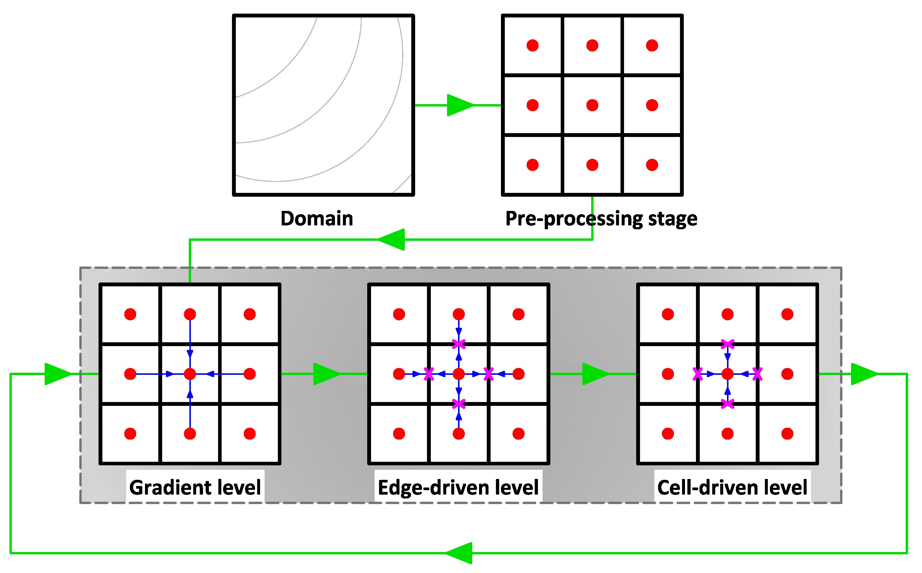
Here we explain in detail how the data structures of our code are designed to advance the solutions of Equation (6). Note this is a typical data structure used in many shallow water codes (with implementations of modern finite volume schemes). As shown in Figure 1, a domain is discretized into several sub-domains (rectangular cells). We call this step the pre-processing stage. Each cell now consists of the values of $z_b$ and $n_m$ located at its center. Initially, the values of h, u, and v are given by users at each cell-center.

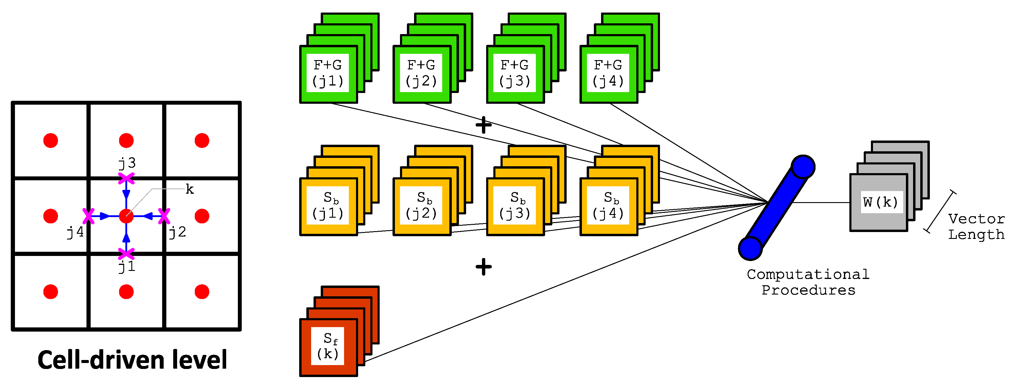
As our model employs a reconstruction process to spatially achieve second-order accuracy with the MUSCL method, it requires the gradient values at cell-center. Therefore, these gradient values must firstly be computed. This step is called the gradient level. Hereafter, one requires to calculate the values at each edge using the values of its two corresponding cell-centers. This stage is then called the edge-driven level. In this level, a solver, e.g., HLLC, Roe, or CU scheme, is required to compute the non-linear values of $\mathbf{F}$ and $\mathbf{G}$ at edges. Prior to performing such a solver, the aforementioned reconstruction process with the MUSCL method was employed. Note the values of ${\mathbf{S}}_b$ are also computed at the edge-driven level. After the values of all edges are known, the solution can be advanced for the subsequent time level by also computing the values of ${\mathbf{S}}_f$. For example, the solutions of $\mathbf{W}$ at the subsequent time level for a cell-center are updated using the $\mathbf{F}$, $\mathbf{G}$, and ${\mathbf{S}}_b$ values from its four corresponding edges—and using ${\mathbf{S}}_f$ values located at the cell-center itself. We call this stage the cell-driven level.

Note that the edge-driven level is the most expensive stage among the others; one should thus pay extra attention to its computation. We also point out here that we apply the computation for the edge-driven level in an edge-based manner rather than in a cell-based one, namely we compute the edge values only once per single calculation level. Therefore, one does not need to save the values of $\left[{\sum }_{i=1}^N{\left(\mathbf{F}{n}_x+\mathbf{G}{n}_y\right)}_i\Delta L_i\right]$ in arrays for each cell-center; only the values of $\left[{\left(\mathbf{F}{n}_x+\mathbf{G}{n}_y\right)}_i\Delta L_i\right]$ are saved corresponding to the total number of edges, instead. The values of an edge are only valid for one adjacent cell—and such values are simply multiplied by ($-1$) for another cell. It is now a challenging task to design an array structure that can ease vectorization and exploit memory access alignment in both the edge-driven and cell-driven levels.

3.2. Cell-Edge Reordering Strategy for Supporting Vectorization and Memory Access Alignment

We focus our reordering strategy here on tackling the two common problems for vectorization: non-contiguous memory access and data-dependency. Regarding the former, a contiguous array structure is required to provide contiguous memory access giving an efficient vectorization. Typically, one finds this problem when dealing with an indirect array indexing, e.g., using $\mathtt{x}\left(\mathtt{y}\right(\mathtt{i}\left)\right)$ forces the compiler to decode $\mathtt{y}\left(\mathtt{i}\right)$ for finding the memory reference of $\mathtt{x}$. This is also a typical problem for a non-unit strided access to array, e.g., incrementing a loop by a scalar factor, where non-consecutive memory locations must be accessed in the loop. The vectorization is sometimes still possible for this problem type. However, the performance gain is often not significant. The second problem relates to usage of arrays identical to the previous iteration of the loop, which often destroy any possibility for vectorization, otherwise a special directive should be used.

See Figure 2, for advancing the solution of $\mathbf{W}$ in Equation (1) for $\mathtt{k}$, one requires $\mathbf{F}$, $\mathbf{G}$, and ${\mathbf{S}}_b$ from $\mathtt{i}$, where $\mathtt{i}=\mathtt{index\_function}\left(\mathtt{j}\right)$ and $[\mathtt{j}\leftarrow \mathtt{1}-\mathtt{4}]$—and ${\mathbf{S}}_f$ from $\mathtt{k}$ itself. Opting $\mathtt{index\_function}$ as an operator for defining $\mathtt{i}$ leads to a use of an indirect reference in a loop. This is not desired since it may avoid the vectorization. This may be anticipated by directly declaring $\mathtt{i}$ into the same array to that of $\mathtt{k}$, e.g., $\mathtt{W}\left(\mathtt{k}\right)\leftarrow \left[\mathtt{W}\right(\mathtt{k}+\mathtt{m}),\mathtt{W}(\mathtt{k}-\mathtt{m}),\mathtt{W}(\mathtt{k}+\mathtt{n}),\mathtt{W}(\mathtt{k}-\mathtt{n}\left)\right]$, where $\mathtt{m}$ and $\mathtt{n}$ are scalar. This, however, leads to a data-dependency problem that makes vectorization difficult.

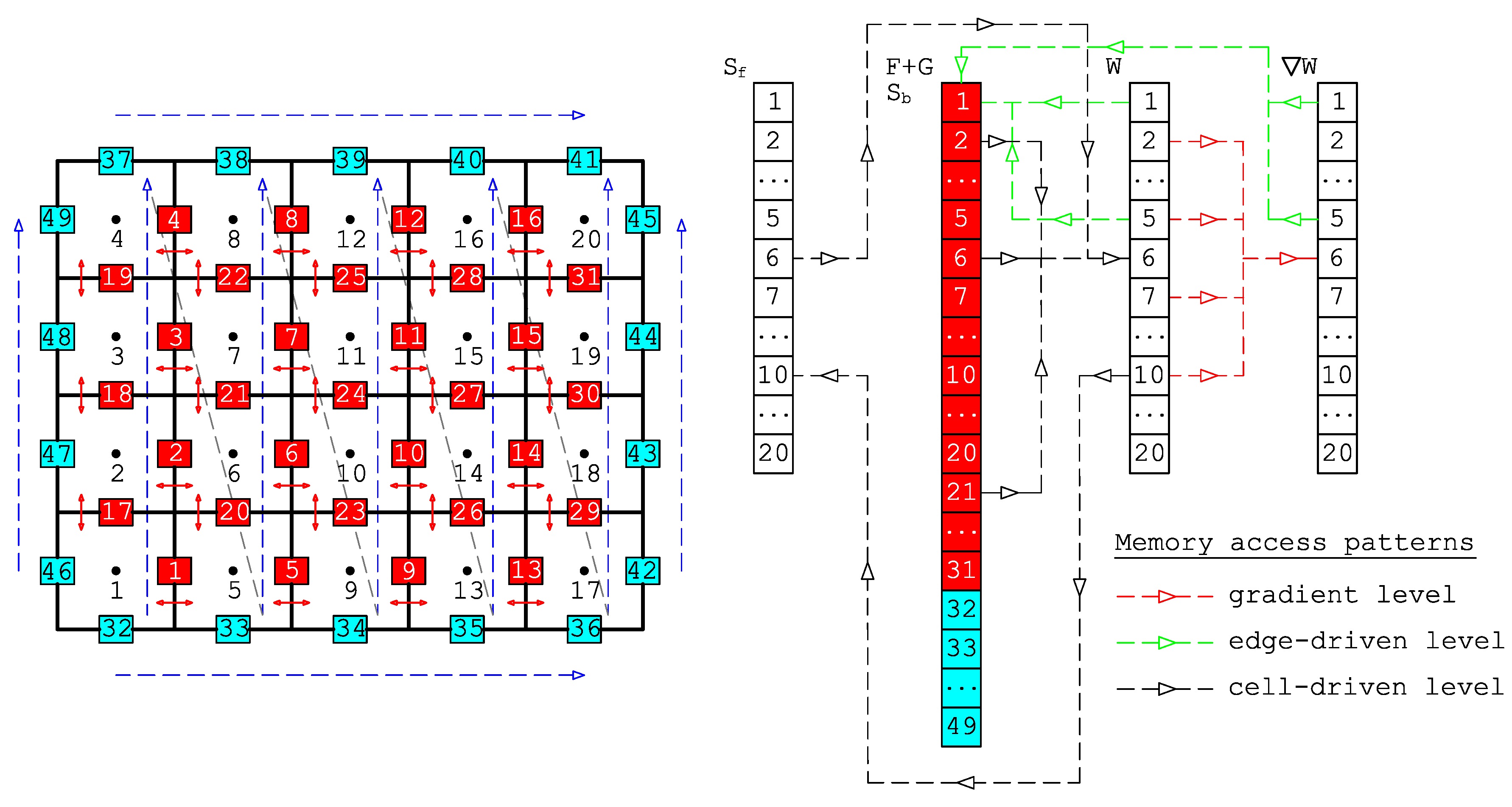
To avoid these problems, we have designed a cell-edge reordering strategy, see Figure 3, where the loops with similar computational procedures are collected to be vectorized. Note that this strategy is only applied once at the pre-processing stage in Figure 1. The core idea of this strategy is to build contiguous array patterns between edges and cells for the edge-driven level as well as between cells and edges for the cell-driven level. We point out here that we only employ 1D array configuration in NUFSAW2D, so that the memory access patterns are straightforward, thus easing unit stride and conserving cache entries. The first step is to devise the cell numbering following the Z-pattern, which is intended for the cell-driven level. Secondly, we design the edge numbering for the edge-driven level by classifying the edges into two types: internal and boundary edges in the most contiguous way; the former is the edges that have two neighboring cells (e.g., edges 1–31), whereas the latter is the edges with only one corresponding cell (e.g., edges 32–49). The reason for this classification is the computational complexity between the internal and boundary edges differs from each other, e.g., (1) no reconstruction process is required for the latter, thus having less CPU time than the former—and (2) due to corresponding to two neighboring cells, the former accesses more memories than does the latter; declaring all edges only in one single loop-group therefore deteriorates the memory access patterns, thus decreasing the performance.

For the sake of clarity, we write in Algorithm 1 the pseudo-code of the model’s $\mathtt{SUBROUTINE}$ employed in NUFSAW2D. Note that Algorithm 1 is a typical form applied in many common and popular shallow water codes. First, we mention that $\mathtt{seg\_x}=\mathtt{5}$, $\mathtt{seg\_y}=\mathtt{4}$, and $\mathtt{Ncells}=\mathtt{20}$ according to Figure 3, where $\mathtt{seg\_x}$, $\mathtt{seg\_y}$, and $\mathtt{Ncells}$ are the total number of domain segments in x and y directions, and the total number of cells, respectively. We now explain the $\mathtt{SUBROUTINE} \mathtt{gradient}$. The cells are now classified into two groups: internal and boundary cells. Internal cells, e.g., cells 6, 7, 10, 11, 14, and 15 are cells whose gradient computations require accessing two cell values in each direction. For example, computing the x-gradient of $\mathbf{W}$ of cell 6 needs the values of $\mathbf{W}$ of cells 2 and 10; this is denoted by $[\nabla {\mathtt{W}}_{\mathtt{x}}\left(\mathtt{6}\right)\leftarrow \mathtt{W}\left(\mathtt{2}\right),\mathtt{W}\left(\mathtt{10}\right)]$ and similarly $[\nabla {\mathtt{W}}_{\mathtt{y}}\left(\mathtt{6}\right)\leftarrow \mathtt{W}\left(\mathtt{5}\right),\mathtt{W}\left(\mathtt{7}\right)]$. Boundary cells, e.g., cells 1–4, 5, 8, 9, 12, 13, 16, and 17–20, are cells affiliated with boundary edges. These cells may not always require accessing two cell values in each direction for the gradient computation, e.g., $[\nabla {\mathtt{W}}_{\mathtt{x}}\left(\mathtt{8}\right)\leftarrow \mathtt{W}\left(\mathtt{4}\right),\mathtt{W}\left(\mathtt{12}\right)]$ but $[\nabla {\mathtt{W}}_{\mathtt{y}}\left(\mathtt{8}\right)\leftarrow \mathtt{W}\left(\mathtt{7}\right),\mathtt{W}\left(\mathtt{8}\right)]$ showing that a symmetric boundary condition is applied to cell 8 in y direction. Considering the fact that the total number of internal cells is significantly larger than that of boundary cells, we group the internal cells into a single loop and distinguish them from the boundary cells, see Algorithm 2.

Algorithm 1 Typical algorithm for shallow water code (within the Runge–Kutta fourth-order (RKFO) method’s framework)

1: for$t=1\leftarrow [\mathtt{total} \mathtt{number} \mathtt{of} \mathtt{time} \mathtt{step}]$do   2:  $!\hspace{1em}\mathtt{within} \mathtt{the} \mathtt{RKFO} \mathtt{method} \mathtt{from}$ [p=1] $\mathtt{to}$ [p=4]   3:  for $p=1\leftarrow 4$ do   4:   $\mathtt{CALL} \mathtt{gradient}$   5:    → $\mathtt{compute} \mathtt{gradient}$   6:   $\mathtt{CALL} \mathtt{edg-driven\_level}$   7:    → $\mathtt{compute} \mathtt{MUSCL\_method}$   8:    → $\mathtt{compute} \mathtt{bed\_slope}$   9:    → $\mathtt{compute} \mathtt{shallow\_water\_solver}$ 10:   $\mathtt{CALL} \mathtt{cell-driven\_level}$ 11:    → $\mathtt{compute} \mathtt{friction\_term}$ 12:    → $\mathtt{compute} \mathtt{update\_variables}$ 13:  end for 14: end for

Algorithm 2 Pseudo-code for $\mathtt{SUBROUTINE} \mathtt{gradient}$

1: for$\mathtt{k}=\mathtt{1}\leftarrow [\mathtt{seg\_x}-\mathtt{2}]$do   2:  $\mathtt{l}=(\mathtt{seg\_y}+\mathtt{2})+(\mathtt{k}-\mathtt{1})\ast \mathtt{seg\_y}$   3:  $\begin{array}{c}\hfill !\$\mathtt{omp} \mathtt{simd} \mathtt{simdlen}\left(\mathtt{VL}\right)\mathtt{aligned}(\nabla {\mathtt{W}}_{\mathtt{x}},\nabla {\mathtt{W}}_{\mathtt{y}}:\mathtt{Nbyte})\end{array}$   4:  for $\mathtt{i}=\mathtt{l}\leftarrow [\mathtt{l}+\mathtt{seg\_y}-\mathtt{3}]$ do   5:   $.........$   6:   $\nabla {\mathtt{W}}_{\mathtt{x}}\left(\mathtt{i}\right)\leftarrow \mathtt{W}(\mathtt{i}-\mathtt{seg\_y}),\mathtt{W}(\mathtt{i}+\mathtt{seg\_y});\nabla {\mathtt{W}}_{\mathtt{y}}\left(\mathtt{i}\right)\leftarrow \mathtt{W}(\mathtt{i}-\mathtt{1}),\mathtt{W}(\mathtt{i}+\mathtt{1})$   7:  end for   8: end for   9: $\begin{array}{c}\hfill !\$\mathtt{omp} \mathtt{simd} \mathtt{simdlen}\left(\mathtt{VL}\right)\mathtt{aligned}(\nabla {\mathtt{W}}_{\mathtt{x}},\nabla {\mathtt{W}}_{\mathtt{y}}:\mathtt{Nbyte})\end{array}$ 10: for$\mathtt{i}=\mathtt{1}\leftarrow \left[\mathtt{seg\_y}\right]$do 11:  $\mathtt{j}=\mathtt{Ncells-seg\_y}+\mathtt{i}$ 12:  $\mathtt{i}\mathtt{1}=\mathtt{i}-\mathtt{1} \mathtt{OR} \mathtt{i}\mathtt{1}=\mathtt{i};\mathtt{i}\mathtt{2}=\mathtt{i}+\mathtt{1} \mathtt{OR} \mathtt{i}\mathtt{2}=\mathtt{i}$ 13:  $\mathtt{i}\mathtt{3}=\mathtt{j}-\mathtt{1} \mathtt{OR} \mathtt{i}\mathtt{3}=\mathtt{j};\mathtt{i}\mathtt{4}=\mathtt{j}+\mathtt{1} \mathtt{OR} \mathtt{i}\mathtt{4}=\mathtt{j}$ 14:  $.........$ 15:  $\nabla {\mathtt{W}}_{\mathtt{x}}\left(\mathtt{i}\right)\leftarrow \mathtt{W}\left(\mathtt{i}\right),\mathtt{W}(\mathtt{i}+\mathtt{seg\_y});\nabla {\mathtt{W}}_{\mathtt{y}}\left(\mathtt{i}\right)\leftarrow \mathtt{W}\left(\mathtt{i}\mathtt{1}\right),\mathtt{W}\left(\mathtt{i}\mathtt{2}\right)$ 16:  $\nabla {\mathtt{W}}_{\mathtt{x}}\left(\mathtt{j}\right)\leftarrow \mathtt{W}(\mathtt{j}-\mathtt{seg\_y}),\mathtt{W}\left(\mathtt{j}\right);\nabla {\mathtt{W}}_{\mathtt{y}}\left(\mathtt{j}\right)\leftarrow \mathtt{W}\left(\mathtt{i}\mathtt{3}\right),\mathtt{W}\left(\mathtt{i}\mathtt{4}\right)$ 17: end for 18: $\begin{array}{c}\hfill !===\mathtt{This} \mathtt{loop} \mathtt{is} \mathtt{not} \mathtt{vectorized} \mathtt{due} \mathtt{to} \mathtt{non-unit} \mathtt{strided} \mathtt{access}===!\end{array}$ 19: for$\mathtt{i}=\mathtt{1}\leftarrow [\mathtt{seg\_x}-\mathtt{2}]$do 20:  $\mathtt{j}=\mathtt{i}\ast \mathtt{seg\_y}+\mathtt{1};\mathtt{k}=(\mathtt{i}+\mathtt{1})\ast \mathtt{seg\_y}$ 21:  $\mathtt{i}\mathtt{1}=\mathtt{j}-\mathtt{1} \mathtt{OR} \mathtt{i}\mathtt{1}=\mathtt{j};\mathtt{i}\mathtt{2}=\mathtt{j}+\mathtt{1} \mathtt{OR} \mathtt{i}\mathtt{2}=\mathtt{j}$ 22:  $\mathtt{i}\mathtt{3}=\mathtt{k}-\mathtt{1} \mathtt{OR} \mathtt{i}\mathtt{3}=\mathtt{k};\mathtt{i}\mathtt{4}=\mathtt{k}+\mathtt{1} \mathtt{OR} \mathtt{i}\mathtt{4}=\mathtt{k}$ 23:  $.........$ 24:  $\nabla {\mathtt{W}}_{\mathtt{x}}\left(\mathtt{j}\right)\leftarrow \mathtt{W}(\mathtt{j}-\mathtt{seg\_y}),\mathtt{W}(\mathtt{j}+\mathtt{seg\_y});\nabla {\mathtt{W}}_{\mathtt{y}}\left(\mathtt{j}\right)\leftarrow \mathtt{W}\left(\mathtt{i}\mathtt{1}\right),\mathtt{W}\left(\mathtt{i}\mathtt{2}\right)$ 25:  $\nabla {\mathtt{W}}_{\mathtt{x}}\left(\mathtt{k}\right)\leftarrow \mathtt{W}(\mathtt{k}-\mathtt{seg\_y}),\mathtt{W}(\mathtt{k}+\mathtt{seg\_y});\nabla {\mathtt{W}}_{\mathtt{y}}\left(\mathtt{k}\right)\leftarrow \mathtt{W}\left(\mathtt{i}\mathtt{3}\right),\mathtt{W}\left(\mathtt{i}\mathtt{4}\right)$ 26: end for

Algorithm 2 shows three typical loops in the $\mathtt{SUBROUTINE} \mathtt{gradient}$. The first loop (lines 1–8) is designed sequentially with a factor of $\mathtt{seg\_x}-\mathtt{2}$ for its outer part to exclude all boundary cells. For its inner part, this loop is constructed based on the outer loop in a contiguous way, thus making vectorization efficient. Each element of array $\nabla {\mathtt{W}}_{\mathtt{x}}$ accesses two elements from array $\mathtt{W}$ with the farthest alignment of $\mathtt{seg\_y}$, while each element of array $\nabla {\mathtt{W}}_{\mathtt{y}}$ also accesses two elements of array $\mathtt{W}$ but only with the farthest alignment of $\mathtt{1}$. The second loop (lines 10–17) is also designed similarly to the first one, but since this loop includes boundary cells, each element of arrays $\nabla {\mathtt{W}}_{\mathtt{x}}$ and $\nabla {\mathtt{W}}_{\mathtt{y}}$ only accesses one array with the farthest alignment of $\mathtt{seg\_y}$ and $\mathtt{1}$, respectively—whereas the other elements from array $\mathtt{W}$ required are contiguously accessed by each element of both $\nabla {\mathtt{W}}_{\mathtt{x}}$ and $\nabla {\mathtt{W}}_{\mathtt{y}}$. Note in our implementation, none of these two loops can be auto-vectorized by the compiler. Therefore, we apply a guided vectorization with OpenMP directive instead of the Intel one, namely $!\$\mathtt{omp} \mathtt{simd} \mathtt{simdlen}\left(\mathtt{VL}\right)\mathtt{aligned}(\mathtt{var}\mathtt{1},\mathtt{var}\mathtt{2},...:\mathtt{Nbyte})$; this will be explained later in Section 4.5. The third loop (lines 19–26) is designed for the rest cells, which are not included in the previous two loops. This loop is not devised in a contiguous manner, thus disabling auto vectorization or, although a guided vectorization is possible, it still does not give any significant performance improvement due to non-unit strided access. Despite being unable to be vectorized, the third loop does not significantly decrease the performance of our model for the entire simulation as it only has an array dimension of $\mathtt{2}\ast [\mathtt{seg\_x}-\mathtt{2}]$ (quite small compared to the other two loops).

We now discuss the $\mathtt{SUBROUTINE} \mathtt{edge-driven\_level}$ and sketch it in Algorithm 3. Note for the sake of brevity, only the pseudo-code for internal edges is represented in Algorithm 3; for boundary edges, the pseudo-code is similar but computed without $\mathtt{MUSCL\_method}$. The first loop corresponds to the edges 1–16 and the second one to the edges 17–31. In the first loop (lines 1–7), each flux computation accesses the array with the farthest alignment of $\mathtt{seg\_y}$, whereas the arrays are designed in the second loop (lines 8–17) to have contiguous patterns. Every edge has a certain pattern for its two corresponding cells, where no data-dependency exists, thus enabling an efficient vectorization. Note with this pattern, both loops can be auto-vectorized; however, we still implement a guided vectorization as it gives a better performance.

Finally, we sketch the $\mathtt{SUBROUTINE} \mathtt{cell-driven\_level}$ in Algorithm 4. Again, for the sake of brevity only the pseudo-code for internal cells is given. Similar to the internal cell in the $\mathtt{SUBROUTINE} \mathtt{gradient}$, the loop is designed sequentially with a factor of $\mathtt{seg\_x}-\mathtt{2}$ for the outer part. In the inner part the arrays access patterns are, however, different to those of the gradient computation, where $\mathtt{W}$ accesses $\mathtt{F}$, $\mathtt{G}$, and ${\mathtt{S}}_{\mathtt{b}}$ from the corresponding edges—and ${\mathtt{S}}_{\mathtt{f}}$ from the corresponding cell; in other words, more array accesses are required in this loop. Nevertheless, the vectorization gives a significant performance improvement since the array accesses patterns are contiguous. However, there is a part that cannot be vectorized in this cell-driven level due to non-unit strided access, similar to that shown in Algorithm 2. Again, since the dimension of this non-vectorizable loop is considerably smaller than the others, there is no significant performance alleviation for the entire simulation.

Algorithm 3 Pseudo-code for $\mathtt{SUBROUTINE} \mathtt{edge-driven\_leve}$ (only for internal edges)

1: $\begin{array}{c}\hfill !\$\mathtt{omp} \mathtt{simd} \mathtt{simdlen}\left(\mathtt{VL}\right)\mathtt{aligned}(\nabla {\mathtt{W}}_{\mathtt{x}},\mathtt{W},{\mathtt{z}}_{\mathtt{b}},\mathtt{F},\mathtt{G},{\mathtt{S}}_{\mathtt{b}}:\mathtt{Nbyte})\end{array}$   2: for$\mathtt{i}=\mathtt{1}\leftarrow [\mathtt{seg\_y}\ast (\mathtt{seg\_x}-\mathtt{1}\left)\right]$do   3:  $\mathtt{j}=\mathtt{i};\mathtt{k}=\mathtt{i}+\mathtt{seg\_y}$   4:  $.........$   5:  $\mathtt{compute} \mathtt{MUSCL\_method}+\mathtt{bed\_slope}+\mathtt{shallow\_water\_solver}$ $\left[\nabla {\mathtt{W}}_{\mathtt{x}}\left(\mathtt{j}\right),\nabla {\mathtt{W}}_{\mathtt{x}}\left(\mathtt{k}\right),\mathtt{W}\left(\mathtt{j}\right),\mathtt{W}\left(\mathtt{k}\right),{\mathtt{z}}_{\mathtt{b}}\left(\mathtt{j}\right),{\mathtt{z}}_{\mathtt{b}}\left(\mathtt{k}\right),...,{{\mathtt{F}}_{\mathtt{x}}}^{\mathtt{L}},{{\mathtt{F}}_{\mathtt{x}}}^{\mathtt{R}},{{\mathtt{G}}_{\mathtt{x}}}^{\mathtt{L}},{{\mathtt{G}}_{\mathtt{x}}}^{\mathtt{R}},{{\mathtt{S}}_{\mathtt{bx}}}^{\mathtt{L}},{{\mathtt{S}}_{\mathtt{bx}}}^{\mathtt{R}}\right]$   6:  $\mathtt{F}+\mathtt{G}\left(\mathtt{i}\right)\leftarrow {{\mathtt{F}}_{\mathtt{x}}}^{\mathtt{L}},{{\mathtt{F}}_{\mathtt{x}}}^{\mathtt{R}},{{\mathtt{G}}_{\mathtt{x}}}^{\mathtt{L}},{{\mathtt{G}}_{\mathtt{x}}}^{\mathtt{R}};{\mathtt{S}}_{\mathtt{b}}\left(\mathtt{i}\right)\leftarrow {{\mathtt{S}}_{\mathtt{bx}}}^{\mathtt{L}},{{\mathtt{S}}_{\mathtt{bx}}}^{\mathtt{R}}$   7: end for   8: for$\mathtt{l}=\mathtt{1}\leftarrow \left[\mathtt{seg\_x}\right]$do   9:  $\mathtt{m}=\mathtt{seg\_y}\ast (\mathtt{seg\_x}-\mathtt{1})+\mathtt{1}+(\mathtt{l}-\mathtt{1})\ast (\mathtt{seg\_y}-\mathtt{1});\mathtt{n}=\mathtt{m}+\mathtt{seg\_y}-\mathtt{2};\mathtt{o}=(\mathtt{l}-\mathtt{1})\ast \mathtt{seg\_y}$ 10:  $\begin{array}{c}\hfill !\$\mathtt{omp} \mathtt{simd} \mathtt{simdlen}\left(\mathtt{VL}\right)\mathtt{aligned}(\nabla {\mathtt{W}}_{\mathtt{y}},\mathtt{W},{\mathtt{z}}_{\mathtt{b}},\mathtt{F},\mathtt{G},{\mathtt{S}}_{\mathtt{b}}:\mathtt{Nbyte})\end{array}$ 11:  for $\mathtt{i}=\mathtt{m}\leftarrow \mathtt{n}$ do 12:   $\mathtt{j}=(\mathtt{i}-\mathtt{m}+\mathtt{1})+\mathtt{o};\mathtt{k}=\mathtt{j}+\mathtt{1}$ 13:   $.........$ 14:   $\mathtt{compute} \mathtt{MUSCL\_method}+\mathtt{bed\_slope}+\mathtt{shallow\_water\_solver}$ $\left[\nabla {\mathtt{W}}_{\mathtt{y}}\left(\mathtt{j}\right),\nabla {\mathtt{W}}_{\mathtt{y}}\left(\mathtt{k}\right),\mathtt{W}\left(\mathtt{j}\right),\mathtt{W}\left(\mathtt{k}\right),{\mathtt{z}}_{\mathtt{b}}\left(\mathtt{j}\right),{\mathtt{z}}_{\mathtt{b}}\left(\mathtt{k}\right),...,{{\mathtt{F}}_{\mathtt{y}}}^{\mathtt{L}},{{\mathtt{F}}_{\mathtt{y}}}^{\mathtt{R}},{{\mathtt{G}}_{\mathtt{y}}}^{\mathtt{L}},{{\mathtt{G}}_{\mathtt{y}}}^{\mathtt{R}},{{\mathtt{S}}_{\mathtt{by}}}^{\mathtt{L}},{{\mathtt{S}}_{\mathtt{by}}}^{\mathtt{R}}\right]$ 15:   $\mathtt{F}+\mathtt{G}\left(\mathtt{i}\right)\leftarrow {{\mathtt{F}}_{\mathtt{y}}}^{\mathtt{L}},{{\mathtt{F}}_{\mathtt{y}}}^{\mathtt{R}},{{\mathtt{G}}_{\mathtt{y}}}^{\mathtt{L}},{{\mathtt{G}}_{\mathtt{y}}}^{\mathtt{R}};{\mathtt{S}}_{\mathtt{b}}\left(\mathtt{i}\right)\leftarrow {{\mathtt{S}}_{\mathtt{by}}}^{\mathtt{L}},{{\mathtt{S}}_{\mathtt{by}}}^{\mathtt{R}}$ 16:  end for 17: end for

Algorithm 4 Pseudo-code for $\mathtt{SUBROUTINE} \mathtt{cell-driven} \mathtt{level}$ (only for internal cells)

1: for$\mathtt{k}=\mathtt{1}\leftarrow [\mathtt{seg\_x}-\mathtt{2}]$do   2:  $\mathtt{j}=(\mathtt{seg\_y}+\mathtt{2})+(\mathtt{k}-\mathtt{1})\ast \mathtt{seg\_y};\mathtt{l}=(\mathtt{seg\_y}\ast (\mathtt{seg\_x}-\mathtt{1})+\mathtt{seg\_y})+(\mathtt{k}-\mathtt{1})\ast (\mathtt{seg\_y}-\mathtt{1})$   3:  $\begin{array}{c}\hfill !\$\mathtt{omp} \mathtt{simd} \mathtt{simdlen}\left(\mathtt{VL}\right)\mathtt{aligned}(\mathtt{W},\mathtt{F},\mathtt{G},{\mathtt{n}}_{\mathtt{m}},{\mathtt{S}}_{\mathtt{b}},{\mathtt{S}}_{\mathtt{f}}:\mathtt{Nbyte})\end{array}$   4:  for $\mathtt{i}=\mathtt{j}\leftarrow [\mathtt{j}+\mathtt{seg\_y}-\mathtt{3}]$ do   5:   $\mathtt{i}\mathtt{1}=\mathtt{l}+(\mathtt{i}-\mathtt{j});\mathtt{i}\mathtt{2}=\mathtt{i};\mathtt{i}\mathtt{3}=\mathtt{i}\mathtt{1}+\mathtt{1};\mathtt{i}\mathtt{4}=\mathtt{i}-\mathtt{seg\_y}$   6:   $.........$   7:   $\mathtt{compute} \mathtt{friction\_term} [\mathtt{W}\left(\mathtt{i}\right),{\mathtt{n}}_{\mathtt{m}}\left(\mathtt{i}\right),...,{\mathtt{S}}_{\mathtt{f}}\left(\mathtt{i}\right)]$   8:   $\mathtt{compute} \mathtt{update\_variables}$   9:   $\mathtt{W}\left(\mathtt{i}\right)\leftarrow \mathtt{F}+\mathtt{G}\left(\mathtt{i}\mathtt{1}\right),\mathtt{F}+\mathtt{G}\left(\mathtt{i}\mathtt{2}\right),\mathtt{F}+\mathtt{G}\left(\mathtt{i}\mathtt{3}\right),\mathtt{F}+\mathtt{G}\left(\mathtt{i}\mathtt{4}\right),{\mathtt{S}}_{\mathtt{b}}\left(\mathtt{i}\mathtt{1}\right),{\mathtt{S}}_{\mathtt{b}}\left(\mathtt{i}\mathtt{2}\right),{\mathtt{S}}_{\mathtt{b}}\left(\mathtt{i}\mathtt{3}\right),{\mathtt{S}}_{\mathtt{b}}\left(\mathtt{i}\mathtt{4}\right),{\mathtt{S}}_{\mathtt{f}}\left(\mathtt{i}\right)$ 10:  end for 11: end for

3.3. Avoiding Skipping Iteration for Vectorization of Wet–Dry Problems

In reality, almost all shallow flow simulations deal with wet–dry problems. To this end, the computations of both solver and bed-slope terms in the $\mathtt{SUBROUTINE} \mathtt{edge-driven} \mathtt{level}$ must satisfy the well-balanced and positivity-preserving properties as well, see [27,28], among others. Similarly, the calculations of the friction terms in the $\mathtt{SUBROUTINE} \mathtt{cell-driven} \mathtt{level}$ must also consider the wet–dry phenomena, otherwise errors are obtained. For example, in the edge-driven level, a wet–dry or dry–dry interface of an edge may exist since one or two cell-centers consist of no water; for both cases, the MUSCL method for achieving second-order accuracy is sometimes not required or even if this method is still computed, it must be turned back to first-order accuracy to ensure computational stability by simply defining the edge values according to the corresponding centers. Another example is in the cell-driven level, where the transformation of the unit discharges ($hu$ and $hv$) back to the velocities (u and v) are required for computing the friction terms by a division of a water depth (h); very low water depth may thus cause significant errors. To anticipate these problems, one often employs some skipping iterations in the loops, see Algorithm 5.

Algorithm 5 Pseudo-code of some possible skipping iterations

1: !== This is a typical skipping iteration in the SUBROUTINE edge-driven level ==!   2: if[wet–dry or dry-dry interfaces at edges]then   3:  NO MUSCL_method: calculate first-order scheme   4: else   5:  compute MUSCL_method: calculate second-order scheme   6:  if [velocities are not monotone] then   7:   back to first-order scheme   8:  end if   9:  $.........$ 10: end if 11: !== This is a typical skipping iteration in the SUBROUTINE cell-driven level ==! 12: if[depths at cell-centers  >  depth limiter] then 13:  compute friction_term 14: else 15:  unit discharges and velocities are set to very small values 16:  $.........$ 17: end if

Typically, the two skipping iterations in Algorithm 5 are important to ensure the correctness of shallow water models. Unfortunately, such layouts may destroy auto vectorization—or although a guided vectorization is possible, it does not give any significant improvement or may even decrease the performance significantly. This is because the SIMD instructions simultaneously work only for sets of arrays, which have contiguous positions. In our experiences, a guided vectorization was indeed possible for both iterations; the speed-up factors, however, were not so significant. Borrowing the idea of [22], we therefore change the layouts in Algorithm 5 to those in Algorithm 6, where the early exit condition is moved to the end of the algorithm. Using the new layouts in Algorithm 6, we significantly observed up to 48% more improvements of the vectorization from those given in Algorithm 5. Note that the results given by Algorithms 5 and 6 should be similar because no computational procedure is changed but only the layouts.

Algorithm 6 Pseudo-code of the solutions of the skipping iterations in Algorithm 5

1: !== A solution for the skipping iteration in the SUBROUTINE edge-driven level ==!   2: compute MUSCL_method: calculate second-order scheme   3: $.........$   4: if[velocities are not monotone]then   5:  back to first-order scheme   6: end if   7: $.........$   8: if[wet–dry or dry-dry interfaces at edges]then   9:  NO MUSCL_method: calculate first-order scheme 10: end if 11: !== A solution for the skipping iteration in the SUBROUTINE cell-driven level ==! 12: compute friction_term 13: $.........$ 14: if[depths at cell-centers   ≤   depth limiter]then 15:  unit discharges and velocities are set to very small values 16:  $.........$ 17: end if

3.4. Parallel Computation

We explain briefly here the parallel computing implementation of NUFSAW2D according to [21]. Our idea is to decompose and parallelize the domain based on its complexity level. NUFSAW2D employs hybrid MPI-OpenMP parallelization, thus is applicable to parallel simulations with multi-nodes. However, as we focus here on the vectorization, which no longer influences the scalability beyond one node [20], we limit our study on single-node implementations and thus only employ OpenMP for parallelization. Further, we examine the memory bandwidth effect when using only one core or 16 cores (AVX), 28 cores (AVX2), and 64 cores (AVX-512).

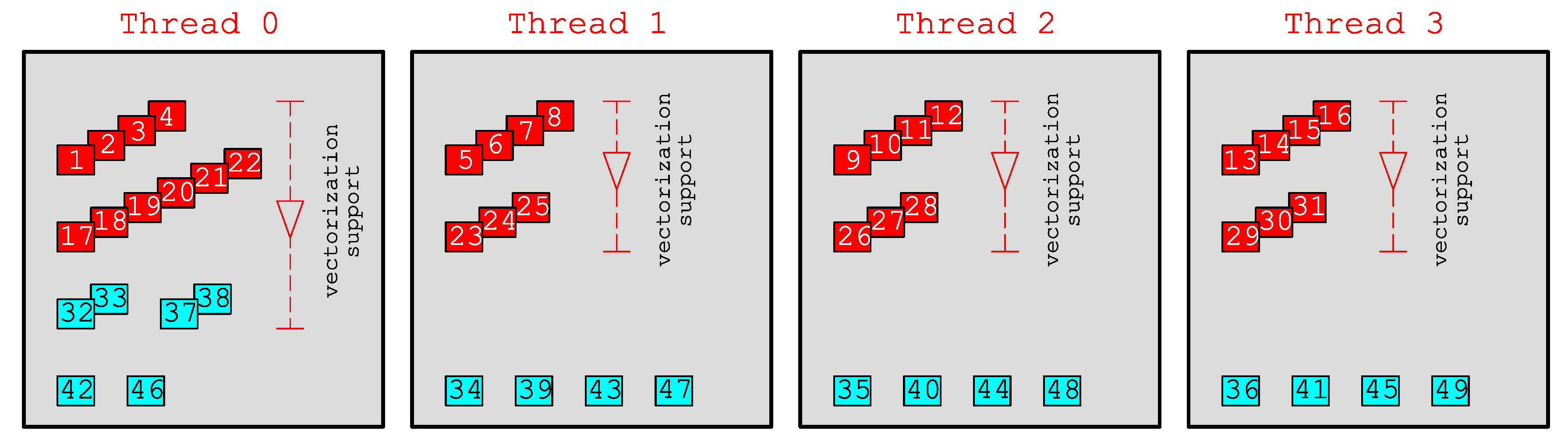
In Figure 4 we show an example of the decomposition of the domain in Figure 3 using four threads; for the sake of brevity, the illustration is given only for the edge-driven level. The parallel directive, e.g., $!\$\mathtt{omp} \mathtt{do}$, can easily be added to each loop, thus according to Algorithm 2, in the gradient level the domain is decomposed as: thread 0 (cells 6, 7, 1, 17, 5, 8), thread 1 (cells 10, 11, 2, 18, 9, 12), thread 2 (cells 14, 15, 3, 19, 13, 16), and thread 3 (cells 4, 20). Similarly, regarding Algorithm 3 it gives in the edge-driven level: thread 0 (edges 1–4, 17–22, 32–33, 37–38, 42, 46), thread 1 (edges 5–8, 23–25, 34, 39, 43, 47), thread 2 (edges 9–12, 26–28, 35, 40, 44, 48), and thread 3 (edges 13–16, 29–31, 36, 41, 45, 49). Meanwhile, the cell-driven level applies a similar decomposition to that of the gradient level. One can see, the largest loop components, e.g., internal edges 1–4, 5–8, etc., are decomposed in a contiguous pattern easing the vectorization implementation, thus efficient. Note the decomposition in Figure 4 is based on static load balancing that causes load imbalance due to the non-uniform amount of loads assigned to each thread; this load imbalance will become less and less significant as the domain size increases, e.g., to millions of cells. However, another load imbalance issue—which can only be recognized during runtime—appears, namely the one caused by wet–dry problems, where wet cells are computationally more expensive than dry cells. For this, we have developed in [21] a novel weighted-dynamic load balancing (WDLB) technique that was proven effective to tackle load imbalance due to wet–dry problems. All the parallel and load balancing implementations are described in detail in [21], thus are not explained here. We also note that we have successfully applied this cell-edge reordering strategy in [24,25] for parallelizing the 2D shallow flow simulations using the CU scheme with good scalability. Yet, we will show in the next section that the cell-edge reordering strategy proposed can help in easing all the vectorization implementations.

4. Results and Discussions

We validate our model against four benchmark tests: two dam-break cases and two tsunami cases. Each case was simulated using a constant $\Delta t$ that satisfies the Courant-Friedrichs-Lewy (CFL) condition, where CFL ≤ 0.5. Our model with the HLLC, Roe, or CU scheme satisfies the well-balanced property; also, the HLLC and CU solvers employed are positivity-preserving. We note that the Roe scheme may in some cases produce negative depths, see [29]; however, in all implementations tested here, we did not find any negative depth with the Roe scheme. The $\Delta t$ used also fulfills the CFL limitation required by the computations of the local one-sided propagation speeds of the CU scheme for positivity-preserving purpose, see [13].

4.1. Case 1: Circular Dam-Break

This case is included to check the capability of our model for symmetry and shock resolution in shallow water flow modeling. We refer to [16,30], among others. A 40 × 40 m, flat, and frictionless domain is considered. A cylindrical wall with a radius of 2.5 m, which was centered at the domain, separated two regions of still water; the first one inside the cylinder had a depth of 2.5 m and the second one outside consisted of 0.5 m water. The water was assumed to be initially at rest and all boundaries were set to wall boundary. The main features to be investigated in this case are the rarefaction wave and the hydraulic jump (shock wave) including a transition condition from subcritical to supercritical flow. The total simulation time was set to 4.7 s with $\Delta t$ = 0.005 s, thus requiring 940 time steps. The domain was discretized into 160,000 rectangular cells (319,200 edges).

The evolutions of the simulated free surface elevation using the CU scheme are visualized in Figure 5. Suddenly after 0.1 s, water started to move in all directions. At 0.4 s, the circular shock wave propagated outwards, whereas the circular rarefaction wave traveled inwards showing that this wave almost reaches the center of the domain. This phenomenon continued until the rarefaction wave has fully plunged into the center of the domain at approximately 0.8 s and this wave was suddenly reflected creating a sharp gradient of water surface elevation. At 1.6 s, the circular shock wave propagated further outwards the from domain center, whereas the reflected rarefaction wave now caused the water to fall below the initial depth of 0.5 m. This produced a secondary circular shock wave, the depth of which was slightly less than 0.5 m. The primary circular shock wave kept propagating outwards the center of the domain at 3.8 s and interestingly, the secondary circular shock wave that had recently been created traveled towards that center. At 4.7 s, it is shown that the primary circular wave almost reached the domain boundary and at this time a very sharp gradient of water surface elevation had been created near that boundary.

We present the comparison between the analytical and numerical results at 4.7 s in Figure 6 showing that all schemes can simulate this highly discontinuous flow properly. To point out the difference between the three schemes more clearly, we present in Figure 7 both the depth and velocity profiles near the two discontinuous areas: 20–22 m and 38–40 m, where only non-significant differences are shown.

4.2. Case 2: Dam-Break Flow against an Isolated Obstacle

This case was done experimentally in [31]. The channel was trapezoidal; 35.8 m long and 3.6 m wide. A 1 m wide rectangular gate separated the upstream reservoir from the downstream channel, see Figure 8. The Manning coefficient was 0.01 $\mathrm{s}{\mathrm{m}}^{-1/3}$. A 0.8 × 0.4 m obstacle was located on the downstream channel with a position that formed an angle of ${64}^o$ from the x-axis. The water was set initially to 0.4 m at the reservoir and 0.02 m at the channel, thus the banks at downstream were dry. The upstream end of the reservoir was a closed wall. In this paper, the domain was discretized into 143,280 rectangular cells (285,246 edges). The simulation was set for 30 s with $\Delta t$ = 0.005 s, thus requiring 6000 time steps.

We compared our model at four points: G1 (10.35, 2.95) m, G4 (11.7, 1.0) m, G5 (12.9, 2.1) m, and G6 (5.83, 2.9) m. Our numerical results are given in Figure 9 showing that our model is in general capable of simulating this case properly. At G1, the maximum bore around 2 s was accurately simulated by all schemes, where there were no significant differences shown until 9 s. However, after 9 s, the CU scheme computed the results higher than do the other schemes, where both the HLLC and Roe schemes show almost no different results. At G4, the first bore around 2 s was predicted with a later time of no more than 1 s and a higher depth of no more than 2 cm, where all schemes kept producing the higher values from 2 s to 4.5 s. At G5, no significant differences were again shown between the HLLC and Roe schemes, but the CU scheme showed slightly different values. At G6, highly accurate results were given by all schemes to simulate the water at the reservoir, showing that the schemes can predict the correct incoming discharge from the upstream reservoir to the downstream channel.

Some errors computed by our model are probably due to the absence of the turbulence terms. Yu and Duan [32] showed the turbulence model was highly important for simulating flow field around the obstacle, where the reflection waves from the obstacle and side walls have superimposed several oblique hydraulic jumps. In Figure 10, we visualize the flood propagation at 1, 3, and 10 s using the CU scheme.

4.3. Case 3: Tsunami Run-Up on a Conical Island

This benchmark case was conducted in a laboratory by [33] to investigate the tsunami run-up on a conical island, the center of which was located near the middle of a 30 × 25 m basin, see Figure 11. To produce planar solitary waves with the specified crest and length, a directional wave maker was used. The left boundary was set as a flow boundary, and the respective water elevation and velocities were defined as

$$\begin{array}{c}\begin{array}{cc}\hfill {\displaystyle \eta (0,y,t)}& =A_e{\sec \mathrm{h}}^2\sqrt{{\displaystyle \frac{3A_e}{4H_e}}}\sqrt{g\left(H_e+A_e\right)}\left(t-T_e\right),\hfill \\ \hfill u(0,y,t)& ={\displaystyle \frac{\eta \sqrt{g\left(H_e+A_e\right)}}{\eta +H_e}},v(0,y,t)=0,\hfill \end{array}\end{array}$$

(7)

where $A_e$, $H_e$, and $T_e$ are the amplitude of the incident wave, still water depth, and time, at which the wave crest enters the domain—set to 0.032 m, 0.32 m, and 2.45 s, respectively. The other three boundaries were closed boundaries. We compared our results with the values at five gauges located on the domain: P-03, P-06, P-09, P-16, and P-22, whose coordinates were (6.82,13.05) m, (9.36, 13.80) m, (10.36, 13.80) m, (12.96, 11.22) m, and (15.56, 13.80) m, respectively. The Manning coefficient was set to zero as suggested by [34].

The domain was discretized into 200,704 rectangular cells (402,304 edges). The simulation time was set to 20 s with $\Delta t$ = 0.002 s leading to 10,000 time steps. One can see in Figure 12, the incident solitary waves in front of the island, which generate a high run-up at about t = 9 s, create wet–dry mechanisms on the conical island. Within this period, the maximum magnitude was reached. After t = 9 s, the waves started to run down the inundated area on the conical island. Some waves were refracted and propagated toward the lee side of the island, where two waves were trapped at each side of the island at around t = 11 s. At t = 13 s, the second wave run-up was generated after these two waves collided. Afterwards, these waves continued to propagate around the island.

Our numerical results are also compared with laboratory results during 20 s, see Figure 13. Accurate results were produced by all schemes, where no significant differences between them were shown. The arrival times of the highest waves were accurately detected at gauges P-03 and P-22. All schemes rendered later times at gauges P-06, P-09, and P-16 but the differences were no more than 1 s. At gauge P-16, our model computed the wave 1 cm higher than the one mentioned in the laboratory data, and the wave at gauge P-22 was computed 1.3 cm higher. This was probably due to the neglect of the dispersion effects. Note that such discrepancies were also reported in the numerical model of [34].

4.4. Case 4: 2011 Japan Tsunami Recorded in Hawaii

This benchmark test is a real tsunami case that occurred in 2011, Japan. The data set was recorded in Hilo Harbor, Hawaii. The raw data can be found in [35]. To avoid the phase differences of the incident wave, the original bathymetry data should be flattened at the depth of 30 m. Interested readers are also referred to [36] for more information. In Figure 14, the sketch of the domain is given as well as the incident wave forcing employed at the northern part as a boundary condition. The Manning coefficient was assumed to be uniform 0.025 $\mathrm{s}{\mathrm{m}}^{-1/3}$. The observation points were the Hilo tide station for elevation (3159, 3472) m, HAI1125/harbor entrance (4686, 2246) m, and HAI1126/inside harbor (1906, 3875) m for velocities. The 1-minute de-tiding of raw data was done for the observed data.

The domain was discretized using 20 m resolution rectangular cells producing 94,600 rectangular cells (189,200 edges). We set the simulation time to 13 h and used $\Delta t$ = 0.025 s giving 1,872,000 time steps. The results are given in Figure 15 plotted per 150 s. At the Hilo tide Station, each scheme can detect the first incoming wave quite accurately around t = 8.2 h. The lowest water elevation was also predicted properly at approximately t = 8.4 h but with a non-significant difference of about 0.2 m. After that, the water level fluctuations were also computed properly. At the harbor entrance, the velocities were in general accurately computed. Each scheme was able to compute the first incoming wave for the x velocity at t = 8.2 h. The y velocity magnitude at that time was, however, slightly overestimated. Inside the harbor, accurate predictions for x and y velocities were shown, where the first incoming wave was well predicted. After 10 h, each scheme kept exhibiting accurate results at the harbor entrance as well as inside the harbor. One can see that the water current flowed predominantly in North–South direction at the harbor entrance, whereas inside the harbor the water current flowed predominantly in East–West direction. Our results agree with the observed data and those simulated by [36] as well. Although some discrepancies—which are probably due to the neglect of the tidal current effects—still exist, our model shows overall quite accurate results for this hazard event.

In Figure 16, the visualizations of tsunami inundation are presented using the CU scheme. It is shown at around 9.03 h, the water level reaches approximately 0.5–1 m at the harbor entrance. Meanwhile, the water level is predicted to reach 1–1.5 m inside the harbor. At about 9.53 h, the water level at the harbor entrance remains relatively constant for 0.5–1 m but outside the harbor (near the breakwater) the water level becomes higher up to 2.5 m. After 14 h, the water level near the breakwater (inside and outside the harbor) decreases to approximately −1.25 m. Complex wet–dry phenomena near the coastline as well as the breakwater appear during the simulation time and our model has shown to be robust for modeling such phenomena.

We show in Figure 17 a visualization of the maximum velocity magnitude captured by the HLLC, Roe, and CU schemes during 13 h simulation time. In general, as one can see, no significant differences are shown between all schemes. Along the outer side of the breakwater as well as near the harbor entrance, the velocity magnitudes of more than 4.5 m/s appear. Meanwhile, considerably lower magnitudes are shown inside the harbor. The main difference is only located near the harbor entrance, where the CU scheme computes the slightly lower magnitudes. The spatial distribution of the velocity magnitude is shown to be extremely sensitive, in agreement with that studied in [36].

4.5. Performance Comparison

We have shown in the previous sections that the HLLC, Roe, and CU schemes are quite accurate for simulating the test cases, where only non-significant differences are shown between them. In this section we analyze and compare the performance of each scheme. All schemes were written and compiled in the same code NUFSAW2D on three machines—AVX (Intel Xeon E5-2690/ Sandy-Bridge-E), AVX2 (Intel Xeon E5-2697 v3/Haswell), and AVX-512 (Intel Xeon Phi/Knights Landing)—for a Linux operating system using Intel Fortran 19. The first computing resource “Sandstorm” was available at our chair [37] and the last two resources “CoolMUC-2” and “CoolMUC-3” were provided by the Leibniz Supercomputing Centre (LRZ) [38]. Each node of the AVX, AVX2, and AVX-512 machines has a total of eight physical cores (16 logical cores), 14 physical cores (28 logical cores), and 64 physical cores, respectively. Note that AVX-512 is built on many-core architecture that incorporates cores with low-frequency and small memory. Therefore, in order to achieve a notable performance, this machine relies on the vector operations on 512 bit SIMD registers.

We did not use the vectorization directive provided by Intel, e.g., $!\mathtt{dir}\$ \mathtt{simd}$, since we have experienced that this directive was not always able to vectorize the loop. Instead, we implemented the directive $!\$\mathtt{omp} \mathtt{simd} \mathtt{simdlen}\left(\mathtt{VL}\right)$ $\mathtt{aligned}(\mathtt{var}\mathtt{1},\mathtt{var}\mathtt{2},...:\mathtt{Nbyte})$ provided by the OpenMP 4.0. The first component ($\mathtt{simdlen}$) was aimed to test the benefit of vectorization on our code compared to the theoretical speed-up based on the vector width, while the second one ($\mathtt{aligned}$) was employed to know the benefit of the aligned memory accesses supported by the reordering strategy proposed. Since we would like to emphasize the effect of vector width, we restricted our discussion here to single-precision arithmetic. The variable $\mathtt{VL}$ was the vector length, set to eight for AVX/AVX2 and 16 for AVX-512—and $\mathtt{Nbyte}$ was the default alignment of the architecture, set to 32 for AVX/AVX2 and 64 for AVX-512.

Two metrics are used to denote the performance of our code: Medge/s/core (million edges per second per core) and Mcell/s/core (million cells per second per core), which are the comparisons between the total number of simulated edges or cells that can be achieved per unit of time using one core. The former was used to denote the performance of the $\mathtt{SUBROUTINE} \mathtt{edge-driven} \mathtt{level}$, whereas the latter was used to denote the performance of the entire simulation. It is also important to note that since the RKFO method is used, the latter is calculated after four times updating per time-level update, not per calculation-level update. We compiled our code using the flag $-\mathtt{O}\mathtt{3} -\mathtt{qopenmp} -\mathtt{align} ’\mathtt{a}’ ’\mathtt{b}’$ for the vectorized version, where $’\mathtt{a}’$ = $\mathtt{array}\mathtt{32}\mathtt{byte}$ for AVX/AVX2 and $\mathtt{array}\mathtt{64}\mathtt{byte}$ for AVX-512—and $’\mathtt{b}’$ = $-\mathtt{xAVX}$ for AVX, $-\mathtt{xCORE}-\mathtt{AVX}\mathtt{2}$ for AVX2, and $-\mathtt{xCOMMON}-\mathtt{AVX}\mathtt{512}$ for AVX-512. To only emphasize the performance increase by vectorization, we disable all possibilities for auto vectorization by compiling with the flag $-\mathtt{O}\mathtt{3} -\mathtt{qopenmp} -\mathtt{no}-\mathtt{vec}-\mathtt{align} ’\mathtt{a}’ ’\mathtt{b}’$ and by deleting all the SIMD directives in the source code, thus giving a fair benchmark of the non-vectorized version of our code.

As previously explained, we discuss our results using single-core and single-node computations. We observed that for single-node computations, NUFSAW2D with OpenMP gives better performance than MPI because the WDLB technique employed for wet–dry problems requires no communication cost. We only performed strong scaling for all cases, where we achieved averagely 87% efficiency for AVX/AVX2 with 16/28 cores and 88% efficiency for AVX-512 with 64 cores. When using 8/16 cores with AVX/AVX2 or 56 cores with AVX-512, higher efficiency was even achieved by our code being approximately 98%. Although this leads to a better performance, we still use the results with all cores available to show the single-node performance. Note the performance degradation of 12–13% (when using all cores) was not due to inefficient load distribution but probably because of the non-uniform memory access (NUMA) effects, where a processor can access its memory faster than the shared non-local memory, see [21].

4.5.1. Performance of Edge-Driven Level

Figure 18 shows the performance comparison between all solvers, in which we observe a significant performance improvement for each solver. Note the results in Figure 18 represent the average values from the four cases tested. We observed that there are no significant differences of the performance (in the range of 4–5%) achieved in all cases. The worst performance was shown in case 2, whereas the best one was achieved in case 1. This is because case 2 deals with more complex wet–dry problems, for which the WDLB technique in this case works better than in the other cases—thus causing more overheads—in order to balance the load units between wet and dry cells, see [21] for detail. For the edge-driven level, each non-vectorized solver shows performance metrics with a range of 3.42–4.54, 5.03–6.23, and 1.01–1.38 Medge/s/core for the AVX, AVX2, and AVX-512, respectively. This shows the CU scheme was, without vectorization, averagely 1.31× and 1.26× faster than the HLLC and Roe solvers, respectively.

As soon the guided vectorization was activated, the performances of each scheme in the edge-driven level increased significantly. For the AVX machine (1 core), we observed significant improvements being 5.5×, 6.5×, and 6× for the HLLC, Roe, and CU schemes, respectively; this shows the Roe scheme experiences remarkably the benefit of the vectorization, for which the improvement factor is larger than the others. For the AVX2 machine (1 core), the speed-up factors of 4.5×, 4.8×, and 5× were obtained by the HLLC, Roe, and CU schemes, respectively showing that the improvement factor of the CU scheme becomes the largest one among the others. Although significant performance improvements have been shown, our model still cannot fully exploit the theoretical speed-up of 8× from the vector widths of both the AVX and AVX2 machines used. Nevertheless, we have shown that the data structures of our code are suitable for SIMD instructions as we are able to achieve the efficiency of up to 81.25%. Note in the aforementioned notable works, none of the models could achieve the performance increase of more than 52% from the theoretical speed-up of the machine used. In [20], the average speed-up of 4.1× was achieved on AVX machine (single-precision) for the vectorized augmented Riemann solver; therefore, this leads to the efficiency of 51.25%. In [22], the average speed-up of 1.7× was obtained on an AVX2 machine (double-precision) for the vectorized Riemann solver; this thus gives the efficiency of 42.5%.

For the AVX-512 machine (1 core), the vectorization has tremendously increased the performances of the HLLC, Roe, and CU solvers by the factors of 16.68×, 16.04×, and 16.42×, respectively. This shows that our model can comprehensively exploit the vectorization for the vector width provided, of which the theoretical speed-up is 16×. Also, this represents that the data structures designed in NUFSAW2D efficiently support the vector programming on this vector-computing architecture.

With parallel simulations, each non-vectorized solver exhibits the performance metrics within the ranges of 2.84–3.78, 4.02–5.11, and 0.81–1.12 Medge/s/core for the AVX (16 cores), AVX2 (28 cores), and AVX-512 (64 cores), respectively; compared to the non-vectorized values with 1 core, it gives about 83% efficiency. For the performance analysis of the parallelized-vectorized solvers, the values obtained by the non-vectorized solvers with single-core are used as indicator. For the AVX machine (16 cores), the parallelized-vectorized HLLC, Roe, and CU solvers reached 16.18, 19.45, and 23.71 Medge/s/core, giving speed-ups of 75.7×, 89.4×, and 83.52×, respectively. Similarly, the parallelized-vectorized HLLC, Roe, and CU solvers obtained 19.45, 21.15, and 27.11 Medge/s/core, respectively with the AVX2 machine (28 cores) leading to speed-ups of 108.4×, 115.6×, and 121.8×. The significant performance increase was shown by the AVX-512 machine (64 cores), where the parallelized-vectorized HLLC, Roe, and CU solvers reached 14.64, 15.36, and 19.98 Medge/s/core, respectively; this brings each scheme to achieve speed-ups of 928.9×, 892.9×, and 924.7×.

The results in Figure 18 show an interesting fact, especially for the single-node performance analysis. Without vectorization, the parallelized results of the AVX2 machine can significantly outperform the parallelized results of the AVX-512 machine. For example, see Figure 19, on the AVX2 machine the CU scheme shows a metric of 143.1 Medge/s with 28 cores while on the AVX-512 machine with 64 cores this scheme exhibits a metric of 71.7 Medge/s; the difference is thus almost two-fold. However, with vectorization, the parallelized results of the AVX2 machine (759.1 Medge/s) are now outperformed by those of the AVX-512 machine (1278.6 Medge/s), being approximately 1.7×. This shows the vectorization is non-trivial for increasing the performance.

Based on these results, one can see although the Roe scheme experiences the largest speed-up on the AVX machine or the HLLC scheme achieves the largest improvement factor on the AVX-512 machine, both of these schemes are still significantly outperformed by the CU scheme with average multiplication factors of 1.4× and 1.25×, respectively. This is not so surprising since the computational procedures of both the HLLC and Roe solvers include complex branch statements ($\mathtt{if-then-else}$), thus should theoretically be much more expensive than the CU scheme, see [17]. The HLLC scheme requires the nested branch statements; the first one is to compute the wave speeds, which are later required in the second branch statement for calculating the final convective fluxes. The Roe scheme needs branchings for the intermediate variables and entropy correction computations, the computations of which are quite complex. Such branchings may force the uses of masked operations and assignments, thus significantly decreasing the performance. In contrast to these two solvers, the CU scheme does not experience any branch statement. This is the beauty of this scheme in addition to being quite simple and having no complex procedure, thus can (even) be auto-vectorized by the compiler.

4.5.2. Performance of the Entire Simulation

Prior to investigating the performance of the entire simulation, we firstly show the cost estimation of each level in Algorithm 1 by presenting in Figure 20 a list of cost percentages: initialization, gradient, edge-driven level and cell-driven level. The last three components indicate the same levels to those shown in Algorithm 1, while initialization is a part required for updating the initial value for the RKFO method per time-level update, e.g., to perform ${\mathbf{W}}^{p=0}={\mathbf{W}}^t$, see Equation (1). Note for an unbiased representative, the values in Figure 20 are the cost percentage of a vectorized solver relatively to its non-vectorized version. Only the cost percentage of the simulations using single-core is presented in Figure 20; the percentage for single-node is shown to be similar. As expected, we observe that the edge-driven level is the most time-consuming part being 65– 75% of the entire simulation for the non-vectorized code. For both AVX and AVX2 machines, the vectorization can decrease the computational cost of the edge-driven level approximately from 71% up to 15%. Meanwhile, for the AVX-512 machine, the vectorization is shown more effective to reduce the cost of the edge-driven level averagely from 72% up to 5%.

The second most expensive part is the cell-driven level, which consumes around 16–22% of the total simulation time with the non-vectorized solvers. After vectorization, the cost of the cell-driven level decreases from approximately 17% up to 5% on both the AVX and AVX2 machines. Meanwhile, on the AVX-512 machine, the vectorization has helped by decreasing the computational time of the cell-driven level averagely from 19% up to 3%; this again shows the vectorization works more effectively on this machine.

We now explain the performance of our model for updating the entire simulation. For the AVX, AVX2, and AVX-512 machines with one core, we observed for the non-vectorized solvers the metrics of 1.27–1.56, 1.78–2.06, and 0.38–0.47 Mcell/s/core, respectively—and for the vectorized solvers by 6.37–7.79, 7.12–9.28, and 5.23–6.23 Mcell/s/core, respectively. We achieved the improvements for the AVX machine by 5×, 5.5×, and 5× for the HLLC, Roe, and CU schemes, respectively, while for the AVX2 machine, the speed-up factors of 4×, 4.5×, and 4.5× were obtained by the HLLC, Roe, and CU schemes, respectively. On the AVX-512 machine we observed the speed-up factors of 13.91×, 13.11×, and 13.18× for the HLLC, Roe, and CU schemes, respectively showing that, on this machine, our code can achieve a better performance than those on the other two machines. However, the AVX2 machine still gives the highest metrics among the others.

For parallel simulations with the AVX, AVX2, and AVX-512 machines, the non-vectorized solvers achieved the metrics of 1.05–1.28, 1.42–1.67, and 0.3–0.38 Mcell/s/core, respectively—and for the parallelized-vectorized solvers by 5.48–6.78, 6.12–8.08, and 4.55–5.48 Mcell/s/core, respectively. Similar to the previous analysis, the values obtained by the non-vectorized solvers with single-core are used as indicator here. According to Figure 21, the vectorized HLLC, Roe, and CU solvers on the AVX machine (16 cores) gave the metrics of 5.48, 6.1, and 6.78 Mcell/s/core reaching speed-ups of 68.8×, 75.68×, and 69.6×, respectively. On the AVX2 machine (28 cores) we observed speed-ups of 96.3×, 108.4×, and 109.6× for the vectorized HLLC, Roe, and CU solvers by obtaining the metrics of 6.12, 6.98, and 8.08 Mcell/s/core, respectively. The AVX-512 machine (64 cores) shows again the significant performance increase by allowing the parallelized–vectorized HLLC, Roe, and CU solvers to achieve the metrics of 4.55, 4.57, and 5.48 Mcell/s/core or similar to speed-ups of 774.6×, 729.9×, and 742.1×, respectively. Based on this fact, a similar behavior is noticed for the single-node performance in updating the entire simulation. We take the results of the CU scheme as an example, see Figure 22. Without vectorization, the parallelized results of the AVX2 machine with 28 cores (46.80 Mcell/s) are about 1.93× significantly faster than those of the AVX-512 machine with 64 cores (24.22 Mcell/s). However, the parallelized–vectorized results of the AVX-512 machine (351 Mcell/s) now outperform the parallelized–vectorized results of the AVX2 machine (226.2 Mcell/s) by a factor of 1.55. This again shows the vectorization is highly-important for achieving better performance. For the entire simulation, our code with the vectorized solvers can achieve approximately 31–35% of the theoretical peak performance (TPP) of the AVX/AVX2 machines and 26% of the TPP of the AVX-512 machine.

We also actually studied the effect of the cell-edge reordering strategy on conserving the memory access patterns, where we compared the directive $!\$\mathtt{omp} \mathtt{simd} \mathtt{simdlen}\left(\mathtt{VL}\right)$ $\mathtt{aligned}(\mathtt{var}\mathtt{1},\mathtt{var}\mathtt{2},...:\mathtt{Nbyte})$ with the directive $!\$\mathtt{omp} \mathtt{simd} \mathtt{simdlen}\left(\mathtt{VL}\right)$. Using the former, we found on all machines that the HLLC, Roe, and CU schemes averagely benefited from 1.45×, 1.5×, 1.4× more speed-ups in the edge-driven level compared to the results compiled only with the latter. Similarly, for updating the entire simulation, the HLLC, Roe, and CU solvers achieved on all machines approximately 1.41×, 1.42×, and 1.32× more speed-ups, respectively. These results reveal that the cell-edge reordering strategy proposed has helped in easing the aligned memory access pattern, thus enabling a significant performance enhancement. For the sake of brevity, these findings are not presented here.

5. Conclusions

A numerical investigation for studying the accuracy and efficiency of three common shallow water solvers (the HLLC, Roe, and CU schemes) has been presented. Four cases dealing with shock waves and wet–dry phenomenon were selected. All schemes were provided in an in-house code NUFSAW2D, the model of which was of second-order accurate in space wherever the regimes were smooth and robust when dealing with strong shock waves—and of fourth-order accurate in time. To give a fair comparison, all source terms of the 2D SWEs were treated similarly for all schemes, namely the bed-slope terms were computed separately from the convective fluxes using a Riemann-solver-free scheme—and the friction terms were computed semi-implicitly within the framework of the RKFO method.

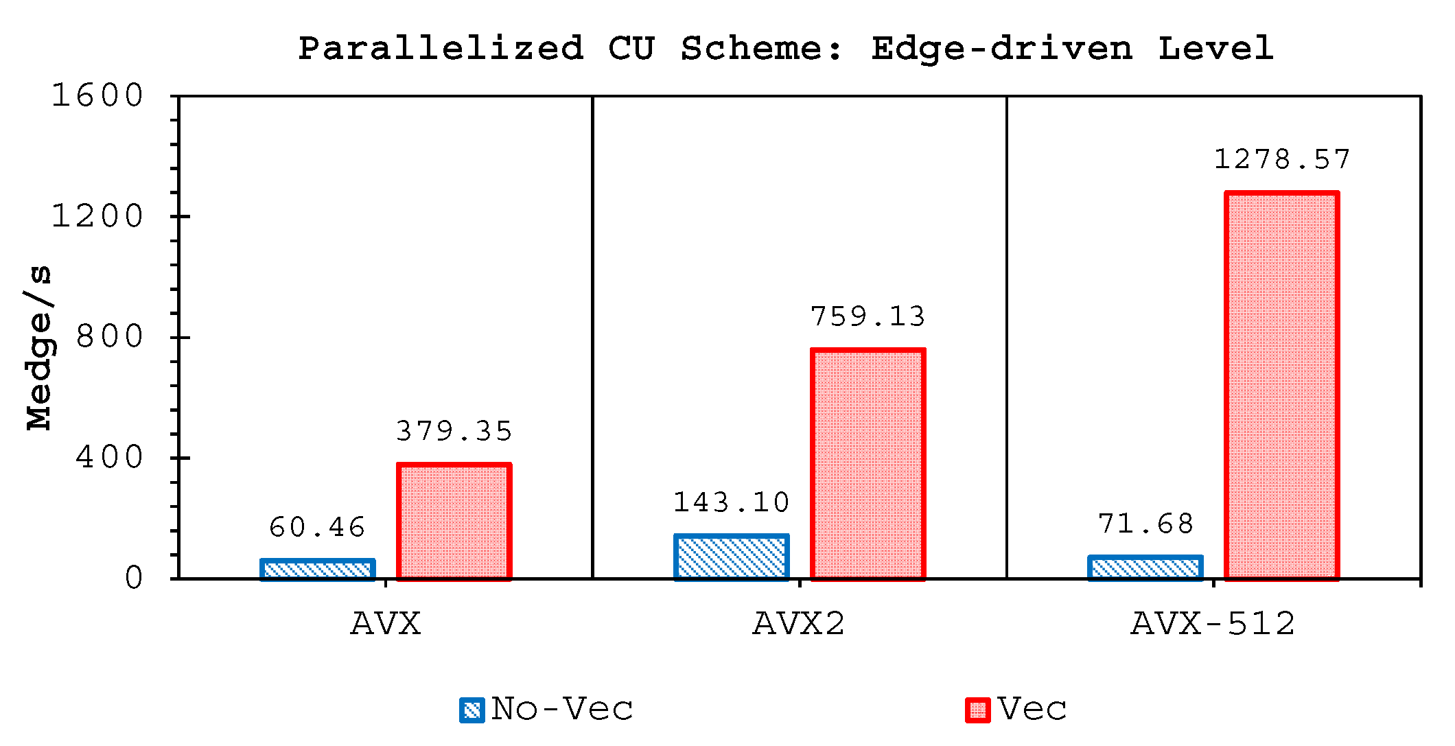
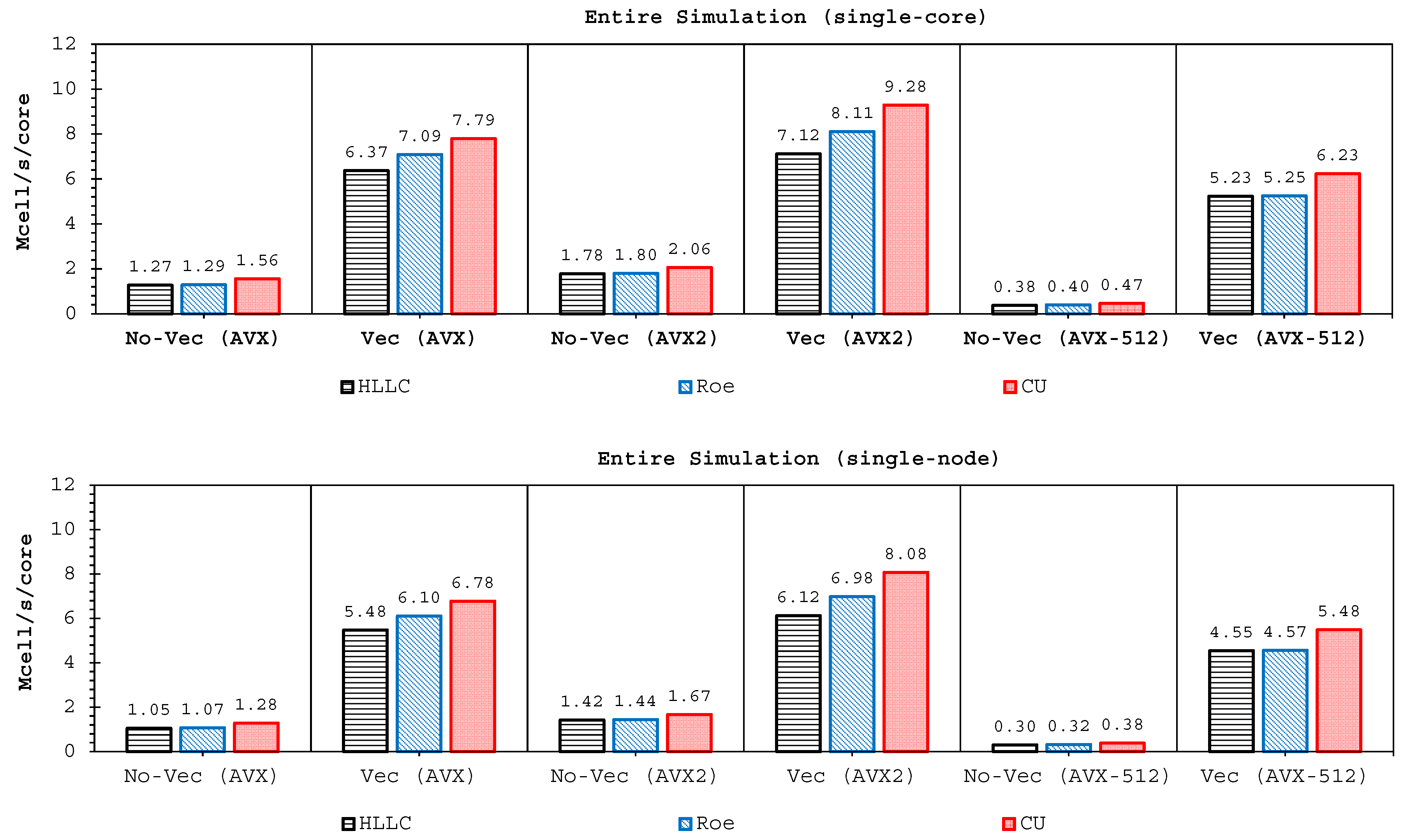
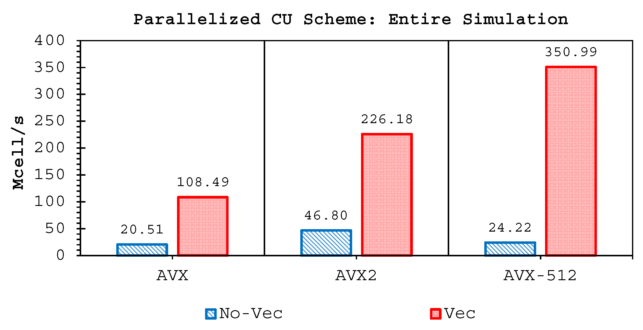
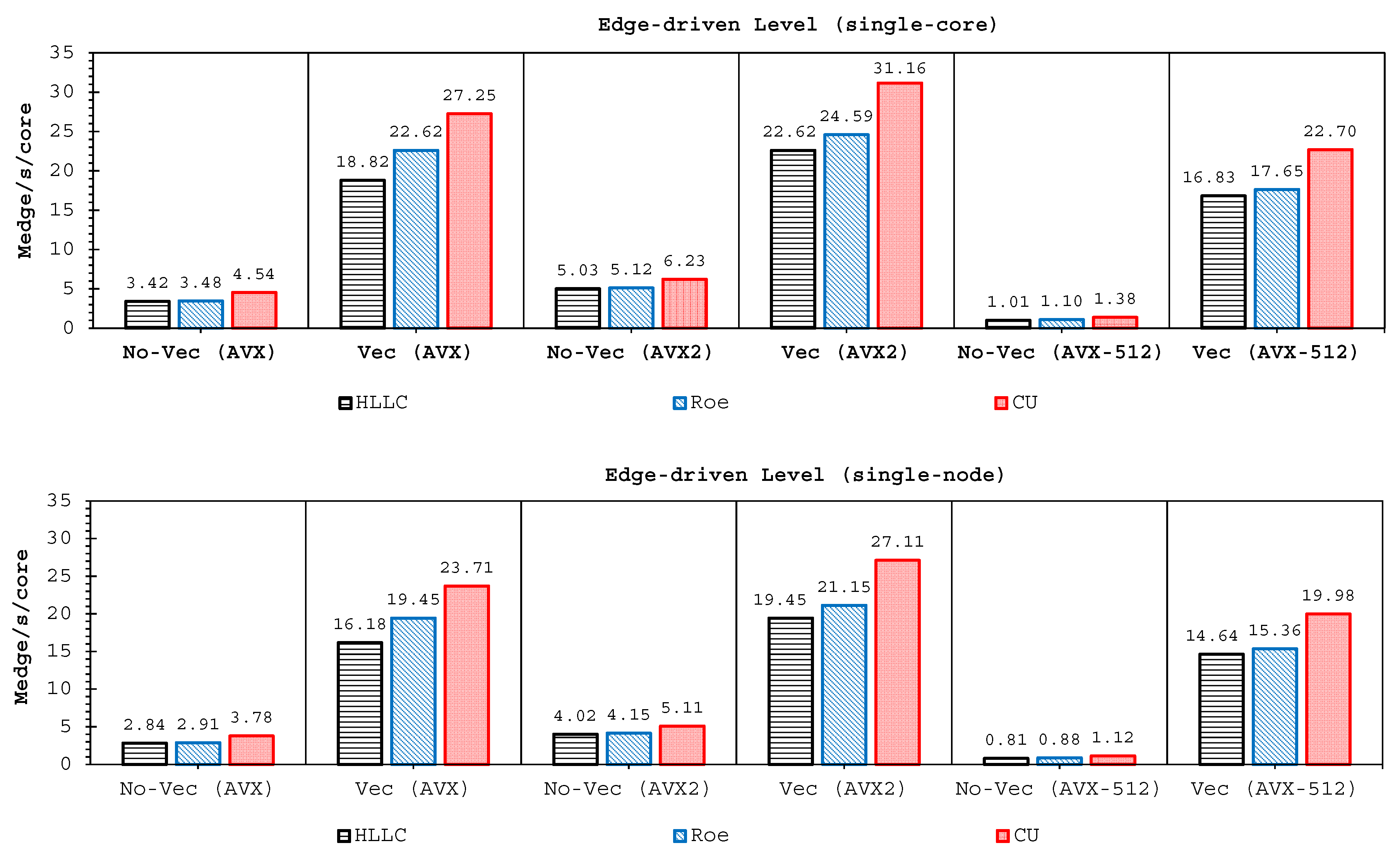
Two important findings have been shown by our simulations. Firstly, highly-efficient vectorization could be applied to the three solvers on all hardware used. This was achieved by guided vectorization, where a cell-edge reordering strategy was employed to ease the vectorization implementations and to support the aligned memory access patterns. Regarding single-core analysis, the vectorization was shown to be able to speed-up the performance of the edge-driven level up to 4.5–6.5× on the AVX/AVX2 machines for eight data per vector and 16.7× on the AVX-512 machine for 16 data per vector—and to accelerate the entire simulation as well by up to 4–5.5× on the AVX/AVX2 machine and 13.91× on the AVX-512 machine. The superlinear speed-up in the edge-driven level especially using the AVX-512 machine could be achieved probably due to improved cache usage, thus less expensive main memory accesses. Regarding single-node analysis, our code could reach in the edge-driven level the improvements of 75.7–121.8× on the AVX/AVX2 machine while on the AVX-512 machine it achieved up to 928.9× speed-up. For updating the entire simulation, our code was able to reach speed-ups of 68.8–109.6× and 774.6× on the AVX/AVX2 and AVX-512 machines, respectively. We observed an interesting phenomenon, where without vectorization the parallelized results of the AVX2 machine outperformed those of the AVX-512 machine in both the edge-driven level and the entire simulation with a factor of up to 2×; the parallelized-vectorized results of the AVX-512 machine became, however, faster by achieving an average factor of 1.6×. This clearly shows that our reordering strategy could efficiently exploit the vectorization support of such a vector-computing machine. Supporting the aligned memory access patterns, the reordering strategy employed has helped in gaining the performances of the “only” vectorized code by averagely 1.45× and 1.4× for the edge-driven level and updating the entire simulation, respectively.

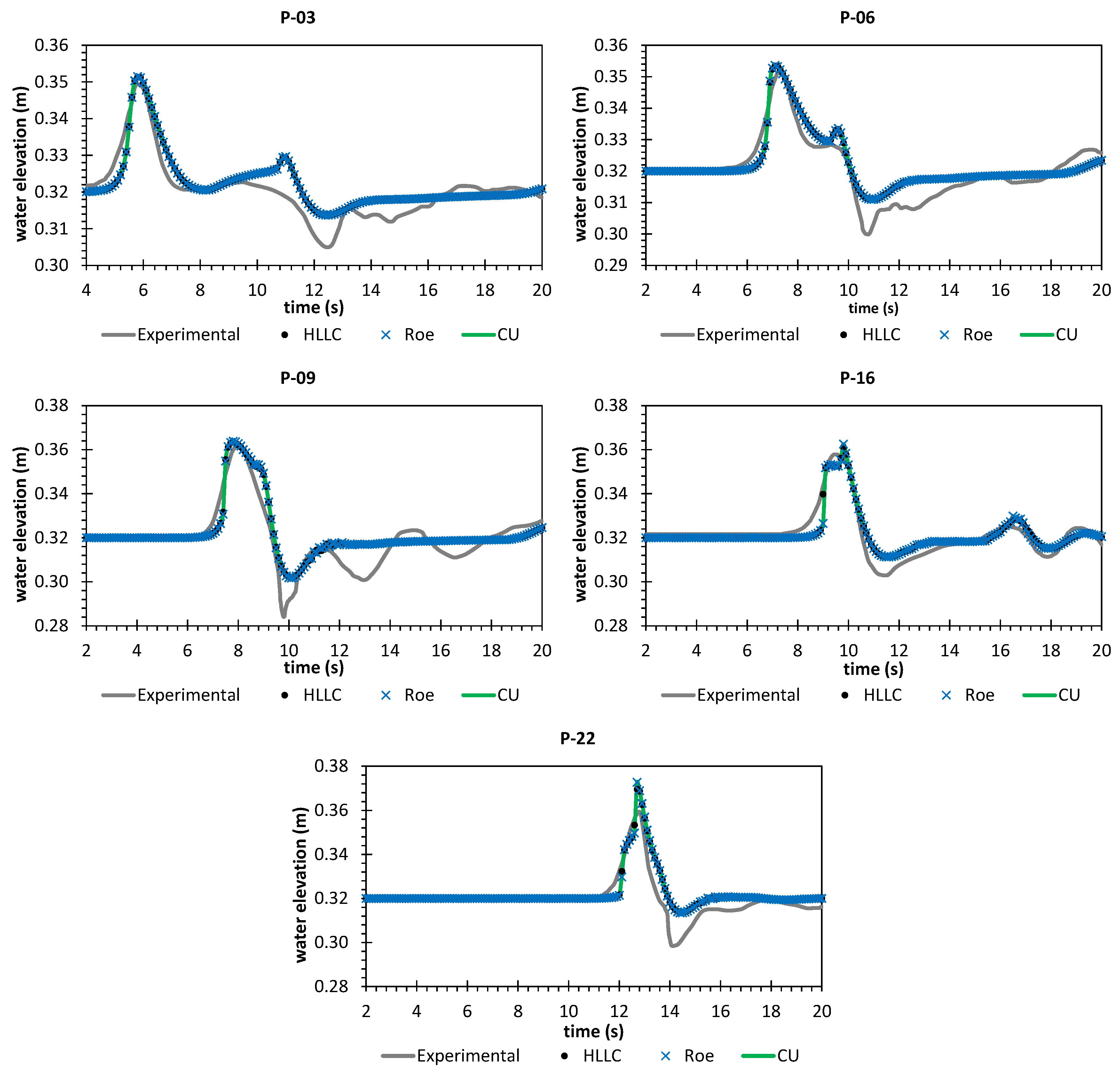
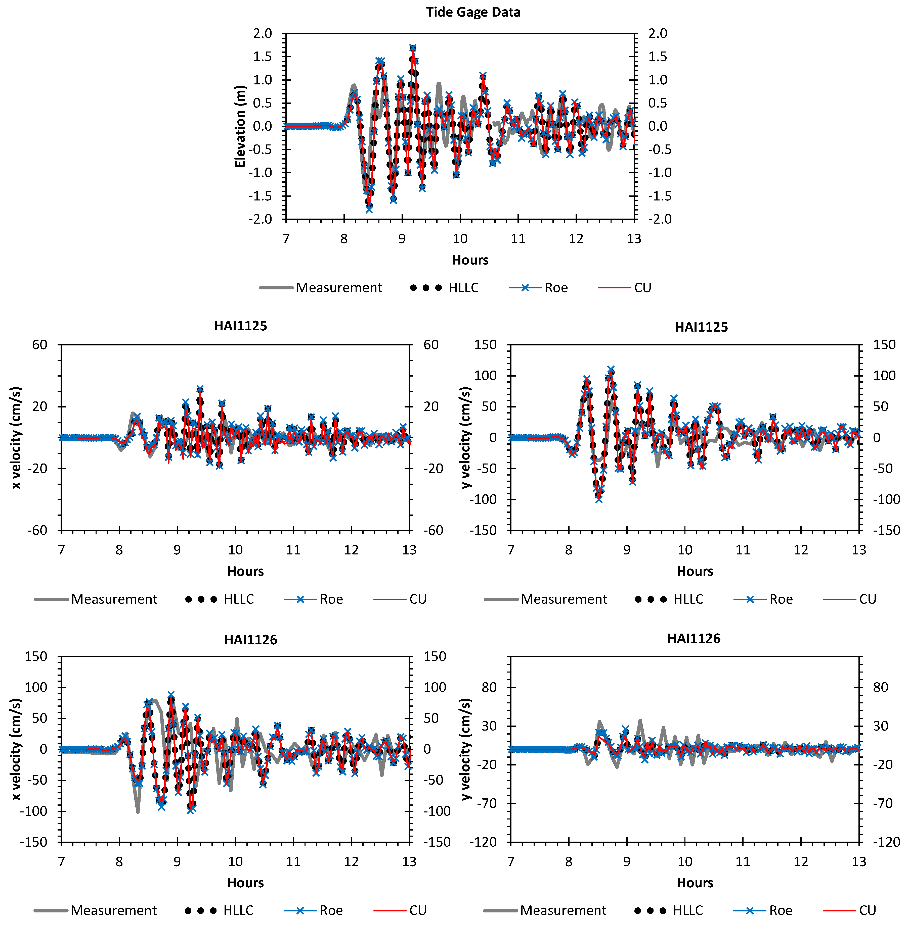
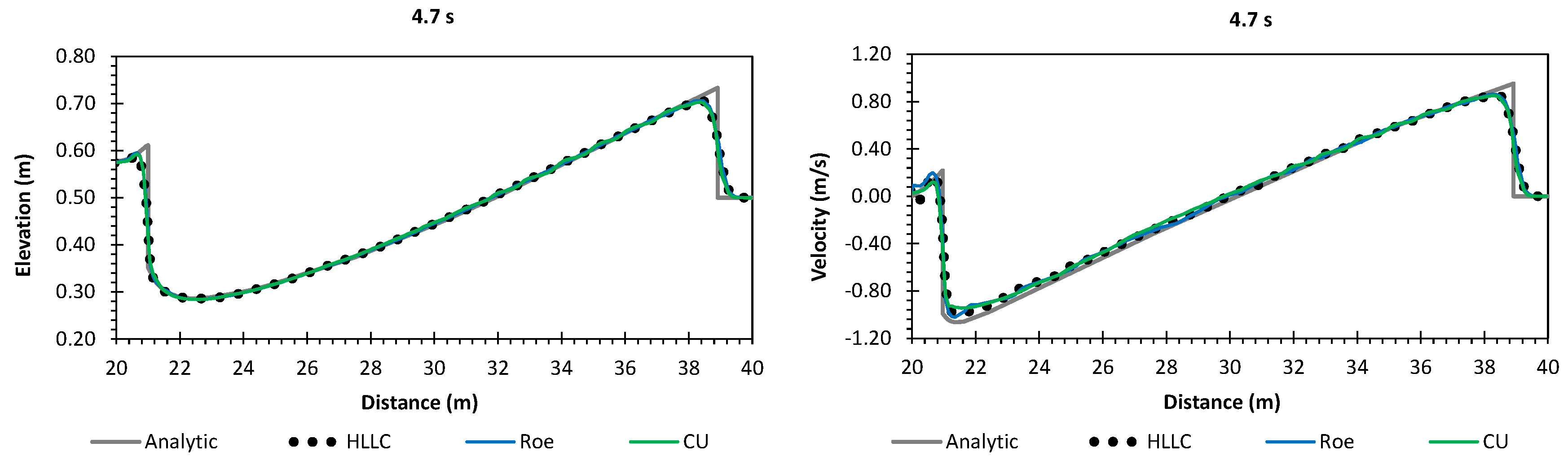
Secondly, we have shown that for the four cases simulated, strong agreements by all schemes were obtained between the numerical results and observed data, where no significant differences were shown for the accuracy. However, in the term of efficiency, the CU scheme was able to outperform the HLLC and Roe schemes with average factors of 1.4× and 1.25×, respectively. Although the vectorization was successful to significantly gain the performance of all solvers, the CU scheme still became the most efficient one among the others. According to this fact, we could conclude that the CU solver as a Riemann-solver-free scheme would in general be able to outperform the Riemann solvers (HLLC and Roe schemes) even for simulations on the next generation of modern hardware. This is because the computational procedures of the CU scheme are acceptably simple especially containing no complex branch statements ($\mathtt{if-then-else}$) such as required by the HLLC and Roe schemes.

Since simulating shallow water flows—especially complex phenomena that require performing long real-time computations as part of disaster planning such as dam-break or tsunami cases—on modern hardware nowadays and even in the future becomes more and more common, focusing simulations only on numerical accuracy but ignoring the performance efficiency is not an option anymore. Wasting the performance is obviously undesirable due to wasting too much time for such long real-time simulations. Modern hardware offers many features for gaining efficiency, one of which is vectorization that can be regarded as the “easiest” way for benefiting from the vector-level parallelism, is thus non-trivial. However, this is not obtained for free; one should at least understand and support—due to the sophisticated memory access patterns—the vectorization concept. The cell-edge reordering strategy employed here is one of the easiest strategies to utilize the vectorization feature of modern hardware that could easily be applied to any CCFV scheme for shallow flow simulations, together with guided vectorization instead of explicitly by low-level vectorization, which might be error-prone and time-consuming. It is worth pointing out that this strategy is also applicable to any compiler with vectorization support, e.g., Gfortran. We observed that the performance obtained with Intel compiler was typically 2–3× higher than that obtained with Gfortran, which we believe is due to the correspondence of Intel compiler and Intel hardware.

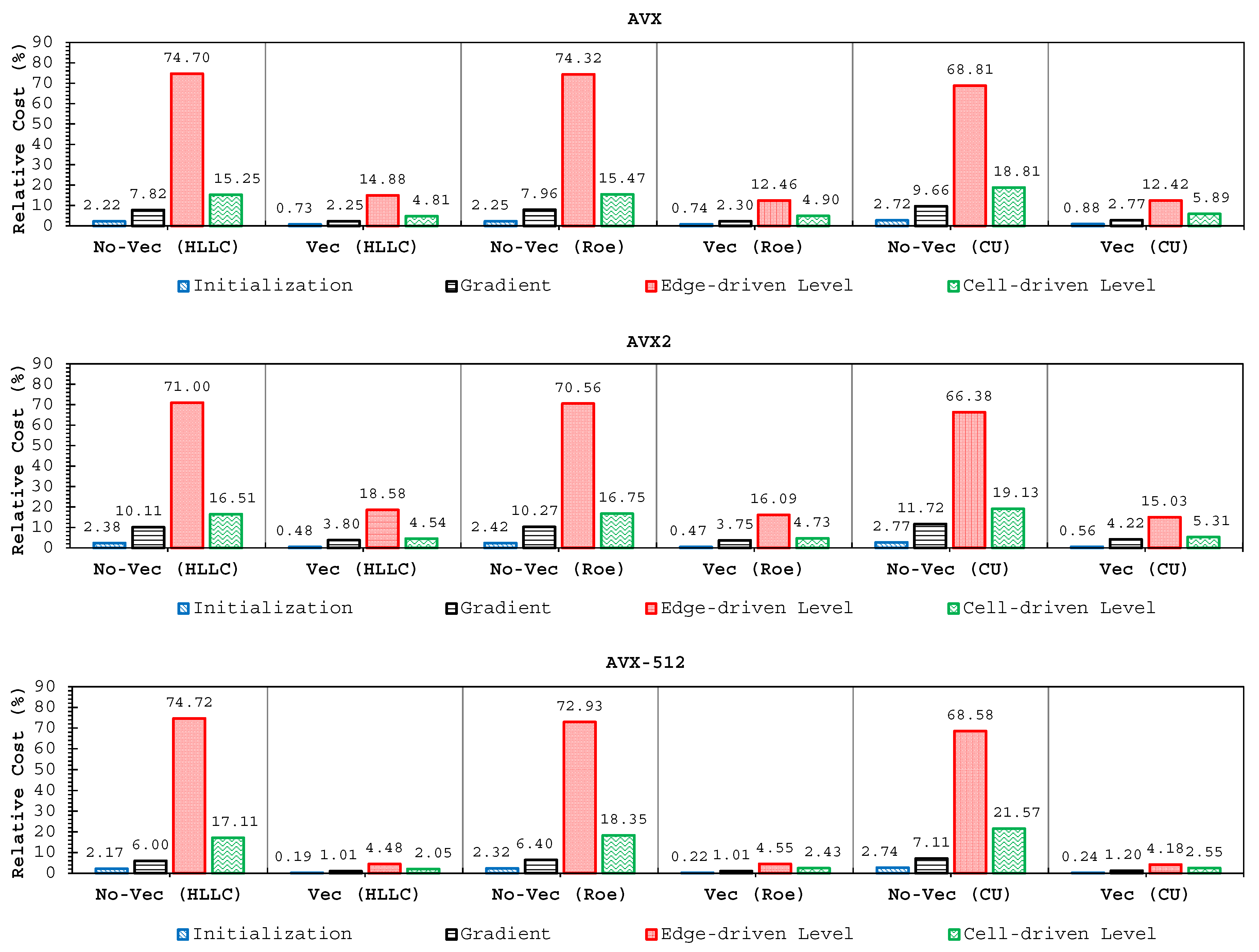
We have also shown that the edge-driven level, especially the reconstruction technique and solver computations, were the most time-consuming part, which required 65–75% of the entire simulation time. This shows that some more “aggressive” optimization techniques still become a hot topic for future studies to make shallow water simulations more efficient, particularly in the edge-driven level. Finally, we conclude that this study would be useful as a consideration for modelers who are interested in developing shallow water codes.

References

1. Cea, L.; Blade, E. A simple and efficient unstructured finite volume scheme for solving the shallow water equations in overland flow applications. Water Resour. Res. 2015, 51, 5464–5486. [Google Scholar] [CrossRef]
2. Hou, J.; Liang, Q.; Zhang, H.; Hinkelmann, R. An efficient unstructured MUSCL scheme for solving the 2D shallow water equations. Environ. Model. Softw. 2015, 66, 131–152. [Google Scholar] [CrossRef]
3. Duran, A. A robust and well-balanced scheme for the 2D Saint-Venant system on unstructured meshes with friction source term. Int. J. Numer. Methods Fluids 2015, 78, 89–121. [Google Scholar] [CrossRef]
4. Özgen, I.; Zhao, J.; Liang, D.; Hinkelmann, R. Urban flood modeling using shallow water equations with depth-dependent anisotropic porosity. J. Hydrol. 2016, 541, 1165–1184. [Google Scholar] [CrossRef]
5. Xia, X.; Liang, Q.; Ming, X.; Hou, J. An efficient and stable hydrodynamic model with novel source term discretization schemes for overland flow and flood simulations. Water Resour. Res. 2017, 53, 3730–3759. [Google Scholar] [CrossRef]
6. Roe, P. Approximate Riemann solvers, parameter vectors and difference schemes. J. Comput. Phys. 1981, 135, 250–258. [Google Scholar] [CrossRef]
7. Toro, E. Shock-Capturing Methods for Free-Surface Shallow Flow; John Wiley: Chichester, UK, 2001. [Google Scholar]
8. Harten, A.; Lax, P.; van Leer, B. On upstream differencing and Godunov-type schemes for hyperbolic conservation laws. SIAM Rev. 1983, 25, 35–61. [Google Scholar] [CrossRef]
9. Davis, S. Simplified second-order Godunov-type methods. SIAM J. Sci. Stat. Comput. 1988, 9, 445–473. [Google Scholar] [CrossRef]
10. Einfeldt, B. On Godunov-type methods for gas dynamics. SIAM J. Numer. Anal. 1988, 25, 294–318. [Google Scholar] [CrossRef]
11. Toro, E.; Spruce, M.; Speares, W. Restoration of the contact surface in the HLL-Riemann solver. Shock Waves 1994, 4, 25–34. [Google Scholar] [CrossRef]
12. Kurganov, A.; Noelle, S.; Petrova, G. Semi-discrete central-upwind schemes for hyperbolic conservation laws and Hamilton-Jacobi equations. SIAM J. Sci. Comput. 1994, 23, 707–740. [Google Scholar] [CrossRef]
13. Kurganov, A.; Petrova, G. A second-order well-balanced positivity preserving central-upwind scheme for the Saint-Venant system. Commun. Math. Sci. 2007, 5, 133–160. [Google Scholar] [CrossRef]
14. Horváth, Z.; Waser, J.; Perdigão, R.; Konev, A.; Blöschl, G. A two-dimensional numerical scheme of dry/wet fronts for the Saint-Venant system of shallow water equations. Int. J. Numer. Methods Fluids 2015, 77, 159–182. [Google Scholar] [CrossRef]
15. Beljadid, A.; Mohammadian, A.; Kurganov, A. Well-balanced positivity preserving cell-vertex central-upwind scheme for shallow water flows. Comput. Fluids 2016, 136, 193–206. [Google Scholar] [CrossRef]
16. Delis, A.; Nikolos, I. A novel multidimensional solution reconstruction and edge-based limiting procedure for unstructured cell-centered finite volumes with application to shallow water dynamics. Int. J. Numer. Methods Fluids 2013, 71, 584–633. [Google Scholar] [CrossRef]
17. Ginting, B.; Mundani, R.P. Artificial viscosity technique: A Riemann-solver-free method for 2D urban flood modelling on complex topography. In Advances in Hydroinformatics; Gourbesville, P., Cunge, J., Caignaert, G., Eds.; Springer Water: Singapore, 2018; pp. 51–74. [Google Scholar]
18. Bik, A.; Girkar, M.; Grey, P.; Tian, X. Automatic intra-register vectorization for the Intel architecture. Int. J. Parallel Program. 2002, 2, 65–98. [Google Scholar] [CrossRef]
19. Nuzman, D.; Rosen, I.; Zaks, A. Auto-vectorization of interleaved data for SIMD. In Proceedings of the 27th ACM SIGPLAN Conference on Programming Language Design and Implementation, Ottawa, ON, Canada, 10–16 June 2006; pp. 132–143. [Google Scholar] [CrossRef]
20. Bader, M.; Breuer, A.; Hölzl, W.; Rettenberger, S. Vectorization of an augmented Riemann solver for the shallow water equations. In Proceedings of the 2014 International Conference on High Performance Computing & Simulation (HPCS), Bologna, Italy, 21–25 July 2014; pp. 193–201. [Google Scholar] [CrossRef]
21. Ginting, B.; Mundani, R.P. Parallel flood simulations for wet-dry problems using dynamic load balancing concept. J. Comput. Civ. Eng. (ASCE) 2019, 33, 1–18. [Google Scholar] [CrossRef]
22. Ferreira, C.; Mandli, K.; Bader, M. Vectorization of Riemann solvers for the single- and multi-layer shallow water equations. In Proceedings of the 2018 International Conference on High Performance Computing & Simulation (HPCS), Orléans, France, 16–20 July 2018; pp. 415–442. [Google Scholar] [CrossRef]
23. Liu, J.Y.; Smith, M.; Kuo, F.A.; Wu, J.S. Hybrid OpenMP/AVX acceleration of a Split HLL finite volume method for the shallow water and Euler equations. Comput. Fluids 2015, 110, 181–188. [Google Scholar] [CrossRef]
24. Ginting, B.; Mundani, R.P.; Rank, E. Parallel simulations of shallow water solvers for modelling overland flows. In Proceedings of the 13th International Conference on Hydroinformatics (HIC 2018), EPiC Series in Engineering, Palermo, Italy, 1–6 July 2018; La Loggia, G., Freni, G., Puleo, V., De Marchis, M., Eds.; Volume 3, pp. 788–799. [Google Scholar] [CrossRef]
25. Ginting, B. Central-upwind scheme for 2D turbulent shallow flows using high-resolution meshes with scalable wall functions. Comput. Fluids 2019, 179, 394–421. [Google Scholar] [CrossRef]
26. Ginting, B. A two-dimensional artificial viscosity technique for modelling discontinuity in shallow water flows. Appl. Math. Model. 2017, 45, 653–683. [Google Scholar] [CrossRef]
27. Audusse, E.; Bouchut, F.; Bristeau, M.O.; Klein, R.; Perthame, B. A fast and stable well-balanced scheme with hydrostatic reconstruction for shallow water flows. SIAM J. Sci. Comput. 2004, 25, 2050–2065. [Google Scholar] [CrossRef]
28. Gallouët, T.; Hérard, J.M.; Seguin, N. Some approximate Godunov schemes to compute shallow-water equations with topography. Comput. Fluids 2003, 32, 479–513. [Google Scholar] [CrossRef]
29. Castro, M.; Gonzales-Vida, J.; Pares, C. Numerical treatment of wet/dry fronts in shallow flows with a modified Roe scheme. Math. Model. Methods Appl. Sci. 2006, 16, 897–931. [Google Scholar] [CrossRef]
30. Yu, H.; Huang, G.; Wu, C. Efficient finite-volume model for shallow-water flows using an implicit dual time-stepping method. J. Hydraul. Eng. (ASCE) 2015, 141, 1–12. [Google Scholar] [CrossRef]
31. Soarez-Frazão, S.; Zech, Y. Experimental study of dam-break flows against an isolated obstacle. J. Hydraul. Res. 2007, 45, 27–36. [Google Scholar] [CrossRef]
32. Yu, C.; Duan, J. Two-dimensional depth-averaged finite volume model for unsteady turbulent flow. J. Hydraul. Res. 2012, 50, 599–611. [Google Scholar] [CrossRef]
33. Briggs, M.; Synolakis, C.; Harkins, G.; Green, D. Laboratory experiments of tsunami runup on a circular island. Pure Appl. Geophys. 1995, 144, 569–593. [Google Scholar] [CrossRef]
34. Nikolos, I.; Delis, A. An unstructured node-centered finite volume scheme for shallow water flows with wet/dry fronts over complex topography. Comput. Methods Appl. Mech. Eng. 2009, 198, 3723–3750. [Google Scholar] [CrossRef]
35. Available online: https://coastal.usc.edu/currents_workshop/index.html (accessed on 25 September 2018).
36. Arcos, M.; LeVeque, R. Validating velocities in the GeoClaw tsunami model using observations near Hawaii from the 2011 Tohoku tsunami. Pure Appl. Geophys. 2014, 17, 849–867. [Google Scholar] [CrossRef]
37. Available online: https://sandstorm.cie.bgu.tum.de/wiki/index.php/Main_Page (accessed on 25 September 2018).
38. Available online: https://www.lrz.de (accessed on 25 September 2018).
Figure 1. Typical process in shallow flow modeling (with implementations of modern finite volume schemes).
Water 11 00639 g001
Figure 2. Vectorization for advancing the solution in the cell-driven level.
Water 11 00639 g002
Figure 3. Cell-edge reordering strategy [21] and an example of memory access patterns.
Water 11 00639 g003
Figure 4. Illustration of load distribution using static load balancing with vectorization support for the edge-driven level based on Figure 3.
Water 11 00639 g004
Figure 5. Case 1: results of the central-upwind (CU) scheme at 0.1, 0.4, 0.8, 1.6, 3.8, and 4.7 s.
Water 11 00639 g005
Figure 6. Case 1: comparison between analytical and numerical results at 4.7 s.
Water 11 00639 g006
Figure 7. Case 1: comparison between analytical and numerical results at 4.7 s (in detail).
Water 11 00639 g007
Figure 8. Case 2: sketch of domain and channel shape.
Water 11 00639 g008
Figure 9. Case 2: comparison of depths between observation and numerical results.
Water 11 00639 g009
Figure 10. Case 2: visualization of the flood propagation at 0, 1, 3, and 10 s using the CU scheme.
Water 11 00639 g010
Figure 11. Case 3: computational domain of solitary wave run-up.
Water 11 00639 g011
Figure 12. Case 3: numerical results using the CU scheme at 9, 11, and 13 s.
Water 11 00639 g012
Figure 13. Case 3: comparison between observation and numerical results.
Water 11 00639 g013
Figure 14. Case 4: bathymetry for simulation and the boundary condition.
Water 11 00639 g014
Figure 15. Case 4: comparison between observation and numerical results.
Water 11 00639 g015
Figure 16. Case 4: visualization of tsunami inundation using the CU scheme at 9.03, 9.53, and 11 h.
Water 11 00639 g016
Figure 17. Case 4: numerical result for the maximum velocity captured during the 13 h simulation time using the Harten-Lax-van Leer-Contact (HLLC), Roe, and CU schemes (top left, top right, bottom).
Water 11 00639 g017
Figure 18. Comparison of performance metrics in the edge-driven level.
Water 11 00639 g018
Figure 19. Single-node performance of the non-vectorized and vectorized CU scheme with parallelization (edge-driven level).
Water 11 00639 g019
Figure 20. Components of the entire simulations for all schemes.
Water 11 00639 g020
Figure 21. Comparison of performance metrics for the entire simulation.
Water 11 00639 g021
Figure 22. Single-node performance of the non-vectorized and vectorized CU scheme with parallelization (entire simulation).
Water 11 00639 g022