Uncertainty in Irrigation Technology: Insights from a CGE Approach


Abstract
1. Introduction
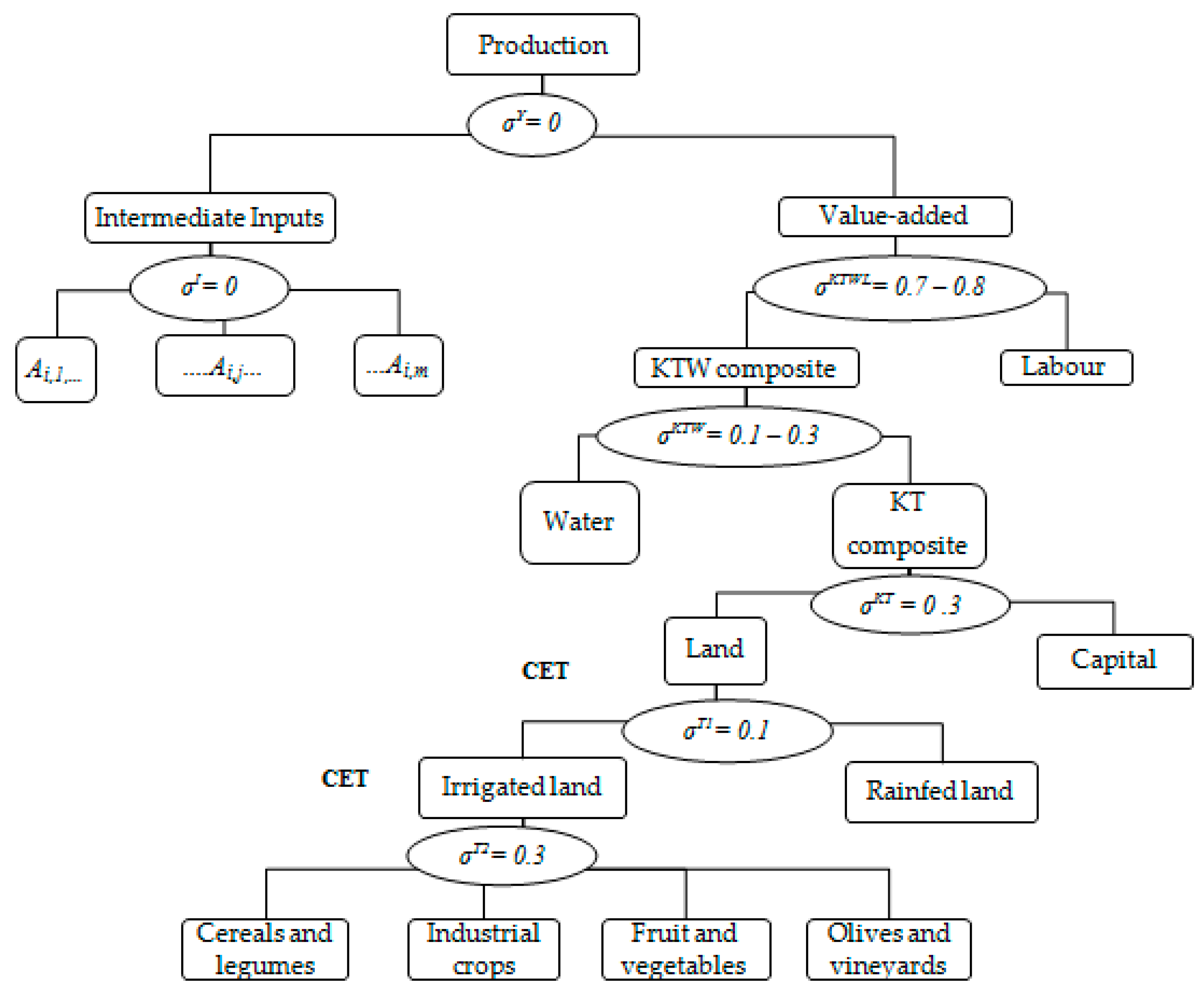
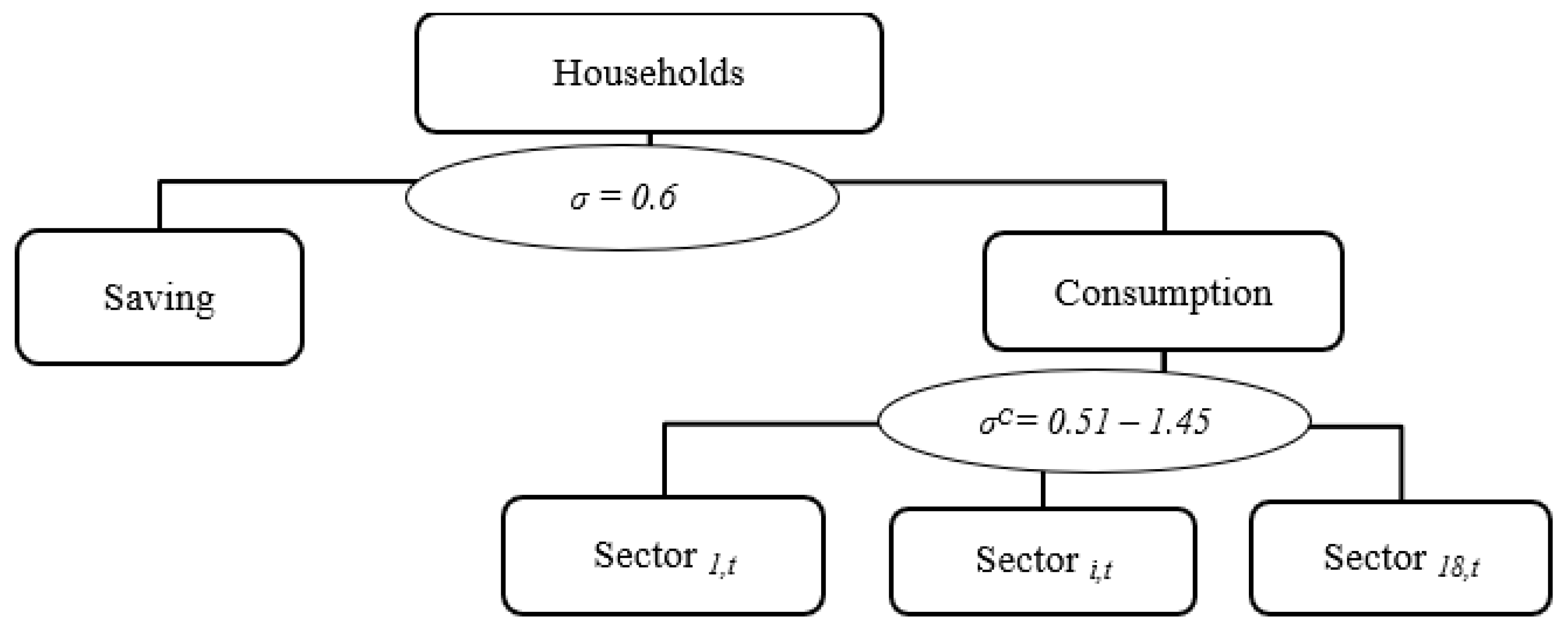
2. The Extended Model
2.1. Outline of the Model
2.2. An Extension to Include Uncertainty in CGE Models
- Scenario 1: The technological improvement never fails, and the five first alternatives (‘2020’, ‘2025’, ‘2030’, ‘2035’, and ‘2040’) are equally likely. This scenario can be identified with a high uncertainty on the date when the top efficiency is achieved as no one has a higher probability than the other, but it is certain that there will be technological progress. We call this uncertainty “high uncertainty”.
- Scenario 2: The technological improvement also never fails, but the five first alternatives follow a discrete stochastic distribution, normal or Gaussian, with the highest probability by ‘2030’—the probabilities are 0.01, 0.21, 0.56, 0.21, and 0.01. It can be identified with a normal distribution of the possible evolutions around the current modernization process which is expected to reach its top efficiency level (at 80%) by 2030. We thus call this uncertainty “normal distribution”.
- Scenario 3: The first five alternatives are equally likely but the large delay; the sixth has a probability of 90%. This level is an arbitrary assumption in order to capture a higher risk of failure in the technological process as an extreme scenario. We call this uncertainty “uncertainty including failure”.
3. Results
4. Concluding Remarks
Supplementary Materials
Author Contributions
Funding
Acknowledgments
Conflicts of Interest
References
- Kwon, C.H.; Chun, B.G. The effect of strategic technology adoptions by local firms on technology spillover. Econ. Model. 2015, 51, 13–20. [Google Scholar] [CrossRef]
- Heal, G.; Kriström, B. Uncertainty and Climate Change. Environ. Resour. Econ. 2002, 22, 3–39. [Google Scholar] [CrossRef]
- Baker, E.; Clarke, L.; Keisler, J.; Shittu, E. Uncertainty, Technical Change, and Policy Models; Technical Report 1028; College of Management, University of Massachusetts: Boston, MA, USA, 2007. [Google Scholar]
- Baker, E.; Shittu, E. Uncertainty and endogenous technical change in climate policy models. Energy Econ. 2008, 30, 2817–2828. [Google Scholar] [CrossRef]
- Qureshi, M.E.; Ahmad, M.; Whitten, S.M.; Kirbyc, M. A multi-period positive mathematical programming approach for assessing economic impact of drought in the Murray–Darling Basin, Australia. Econ. Model. 2014, 39, 293–304. [Google Scholar] [CrossRef]
- Luo, J.L.; Hu, Z.H. Risk paradigm and risk evaluation of farmers cooperatives’ technology innovation. Econ. Model. 2015, 44, 80–85. [Google Scholar] [CrossRef]
- Batabyal, A.A.; Belad, B. The effects of probabilistic innovations on Schumpeterian economic growth in a creative region. Econ. Model. 2016, 53, 224–230. [Google Scholar] [CrossRef]
- Poudel, B.N.; Paudel, K.P. An integrated approach to analyzing risk in bioeconomic models. Nat. Res. Model. 2018, 31, e12172. [Google Scholar] [CrossRef]
- Philip, J.M.; Sánchez-Chóliz, J.; Sarasa, C. Technological change in irrigated agriculture in a semi-arid region of Spain. Water Resour. Res. 2014, 50, 9221–9235. [Google Scholar] [CrossRef]
- Sánchez-Chóliz, J.; Sarasa, C. River Flows in the Ebro Basin: A Century of Evolution, 1913–2013. Water 2015, 7, 3072–3082. [Google Scholar] [CrossRef]
- Arrow, K.J.; Debreu, G. Existence of an Equilibrium for a Competitive Economy. Econometrica 1954, 22, 265–290. [Google Scholar] [CrossRef]
- Harrison, G.W.; Jensen, S.E.H.; Pedersen, L.H.; Rutherford, T.F. (Eds.) Using Dynamic General Equilibrium Models for Policy Analysis; North-Holland: Amsterdam, The Netherlands, 2000. [Google Scholar]
- Gerlagh, R.; Van der Zwaan, B.C.C. Gross world product and consumption in a global warming model with endogenous technological change. Resour. Energy Econ. 2003, 25, 35–57. [Google Scholar] [CrossRef]
- Dellink, R.; Van Ierland, E. Pollution abatement in the Netherlands: A dynamic applied general equilibrium assessment. J. Policy Model. 2006, 28, 207–221. [Google Scholar] [CrossRef]
- Böhringer, C.; Löschel, A.; Moslener, U.; Rutherford, T.F. EU climate policy up to 2020: An economic impact assessment. Energy Econ. 2009, 31 (Suppl. 2), S295–S305. [Google Scholar] [CrossRef]
- González-Eguino, M. The importance of the design of market-based instruments for CO2 mitigation: An AGE analysis for Spain. Ecol. Econ. 2011, 70, 2292–2302. [Google Scholar] [CrossRef]
- Elshennawy, A.; Robinson, S.; Willenbockel, D. Climate change and economic growth: An intertemporal general equilibrium analysis for Egypt. Econ. Model. 2016, 52, 681–689. [Google Scholar] [CrossRef]
- Gómez, C.M.; Tirado, D.; Rey-Maquieira, J. Water exchanges versus water works: Insights from a computable general equilibrium model for the Balearic Islands. Water Resour. Res. 2004, 40, 1–11. [Google Scholar] [CrossRef]
- Velázquez, E.; Cardenete, M.A.; Hewings, G.J.D. Precio del agua y relocalización sectorial del recurso en la economía andaluza. Una aproximación desde un modelo de equilibrio general aplicado. Estud. Econ. Apl. 2006, 24, 3. [Google Scholar]
- Berrittella, M.; Hoekstra, A.Y.; Rehdanz, K.; Roson, R.; Tol, R.S.J. The economic impact of restricted water supply: A computable general equilibrium analysis. Water Res. 2007, 41, 1799–1813. [Google Scholar] [CrossRef]
- Brower, R.; Hofkes, M.; Linderhof, V. General equilibrium modelling of the direct and indirect economic impacts of water quality improvements in the Netherlands at national and river basin scale. Ecol. Econ. 2008, 66, 127–140. [Google Scholar] [CrossRef]
- Van Heerden, J.H.; Blignaut, J.; Horridge, M. Integrated water and economic modelling of the impacts of water market instruments on the South African economy. Ecol. Econ. 2008, 66, 105–116. [Google Scholar] [CrossRef]
- Calzadilla, A.; Rehdanz, K.; Tol, R.S.J. Water scarcity and the impact of improved irrigation management: A computable general equilibrium analysis. Agric. Econ. 2011, 42, 305–323. [Google Scholar] [CrossRef]
- Calzadilla, A.; Rehdanz, K.; Roson, R.; Sartori, M.; Tol, R.S.J. The WSPC reference on natural resources and environmental policy in the era of global change. In Review of CGE Models of Water Issues; Bryant, T., Ed.; World Scientific: Singapore, 2017; pp. 101–124. ISBN 9789814713740. [Google Scholar]
- Brower, R.; Hofkes, M. Integrated hydro-economic modelling: Approaches, key issues and future research directions. Ecol. Econ. 2008, 66, 16–22. [Google Scholar] [CrossRef]
- Böhringer, C.; Löschel, A. Computable general equilibrium models for sustainability impact assessments: Status quo and prospects. Ecol. Econ. 2006, 60, 49–64. [Google Scholar] [CrossRef]
- Pratt, S.; Blake, A.; Swann, P. Dynamic general equilibrium model with uncertainty: Uncertainty regarding the future path of the economy. Econ. Model. 2013, 32, 429–439. [Google Scholar] [CrossRef]
- Böhringer, C.; Rutherford, T.F. Innovation, uncertainty and instrument choice for climate policy. In Proceedings of the the Annual Congress of the Verein für Socialpolitik, Munich, Germany, October 2007. [Google Scholar]
- Durand-Lasserve, O.; Pierru, A.; Smeers, Y. Uncertain long-run emissions targets, CO2 price and global energy transition: A general equilibrium approach. Energy Policy 2010, 38, 5108–5122. [Google Scholar] [CrossRef]
- Babiker, M.; Gurgel, A.; Paltsev, S.; Reilly, J. Forward-looking versus recursive-dynamic modeling in climate policy analysis: A comparison. Econ. Model. 2009, 26, 1341–1354. [Google Scholar] [CrossRef]
- Silvestre, J.; Clar, E. The demographic impact of irrigation projects: A comparison of two case studies of the Ebro basin, Spain, 1900–2001. J. Hist. Geogr. 2010, 36, 315–326. [Google Scholar] [CrossRef]
- Sánchez-Chóliz, J.; Sarasa, C. Water resources analysis in Riegos del Alto Aragón (Huesca) in the first decade of the 21st century. Econ. Agrar. Recur. Nat. 2013, 13, 95–122. [Google Scholar] [CrossRef]
- Berck, P.; Robinson, S.; Goldman, G.E. The Use of Computable General Equilibrium Models to Assess Water Policies; Department of Agricultural & Resource Economics, UC Berkeley: Berkeley, CA, USA, 1991. [Google Scholar]
- Goodman, D.J. More Reservoirs or Transfers? A Computable General Equilibrium Analysis of Projected Water Shortage in the Arkansas River Basin. J. Agric. Resour. Econ. 2000, 25, 698–713. [Google Scholar]
- Banse, M.; van Meijl, H.; Tabeau, A.; Woltjer, G. Will EU biofuel policies affect global agricultural markets? Eur. Rev. Agric. Econ. 2008, 35, 117–141. [Google Scholar] [CrossRef]
- Birur, D.; Hertel, T.; Tyner, W. Impact of Biofuel Production on World Agricultural Markets: A Computable General Equilibrium Analysis; GTAP Working Paper no. 53; Center for Global Trade Analysis, Purdue University: West Lafayette, IN, USA, 2008. [Google Scholar]
- Yang, J.; Huang, J.; Qiu, H.; Rozelle, S.; Sombilla, M.A. Biofuels and the Greater Mekong Subregion: Assessing the impacts on prices, production and trade. Appl. Energy 2009, 86, 37–46. [Google Scholar] [CrossRef]
- Armington, P. A theory of demand for products distinguished by place of production. Int. Monet. Fund Staff Pap. 1969, 19, 159–178. [Google Scholar] [CrossRef]
- Rutherford, T.F.; Meeraus, A. Mixed complementarity formulations of stochastic equilibrium models with recourse. In Proceedings of the GOR Workshop “Optimization under Uncertainty”, Bad Honnef, Germany, 20–21 October 2005. [Google Scholar]
- Rutherford, T.F. Applied general equilibrium modeling with MPSGE as a GAMS subsystem: An overview of the modeling framework and syntax. Comput. Econ. 1999, 14, 1–46. [Google Scholar] [CrossRef]
- MAGRAMA. 2008 Horizon National Irrigation Plan; Ministry of Agriculture Food and Environment: Madrid, Spain, 2008. [Google Scholar]
- Cazcarro, I.; Duarte, R.; Sánchez-Chóliz, J.; Sarasa, C. Water Rates and the Responsibilities of Direct, Indirect and End-Users in Spain. Econ. Syst. Res. 2011, 23, 409–430. [Google Scholar] [CrossRef]
- Sarasa, C. Irrigation Water Management: An Analysis Using Computable General Equilibrium Models. Ph.D. Thesis, University of Zaragoza, Zaragoza, Spain, 2014. [Google Scholar]


| Without Modernization | With Modernization | |||||||||||||||||||
|---|---|---|---|---|---|---|---|---|---|---|---|---|---|---|---|---|---|---|---|---|
| Period | % Difference Compared to the Base Period | Percentage-Points Difference between Non-Modernization and Modernization | ||||||||||||||||||
| Impact of Declining Water Supply | Scenario 1 | Scenario 2 | Scenario 3 | |||||||||||||||||
| Year in which the 80% level of efficiency is reached and expected values | ||||||||||||||||||||
| ‘2020’ | ‘2025’ | ‘2030’ | ‘2035’ | ‘2040’ | Expected Values | ‘2020’ | ‘2025’ | ‘2030’ | ‘2035’ | ‘2040’ | Expected values | ‘2020’ | ‘2025’ | ‘2030’ | ‘2035’ | ‘2040’ | ‘2100’ | Expected Values | ||
| 2002–2010 | −8.52 | 5.97 | 4.90 | 3.97 | 3.35 | 3.05 | 4.25 | 5.97 | 4.90 | 3.97 | 3.35 | 3.05 | 4.04 | 5.96 | 4.89 | 3.96 | 3.34 | 3.04 | 0.96 | 1.29 |
| 2011–2019 | −18.48 | 12.39 | 10.84 | 9.36 | 8.29 | 7.51 | 9.68 | 12.39 | 10.84 | 9.36 | 8.29 | 7.51 | 9.46 | 12.41 | 10.85 | 9.37 | 8.30 | 7.52 | 2.26 | 3.00 |
| 2020–2028 | −29.16 | 15.53 | 14.16 | 12.69 | 11.55 | 10.61 | 12.91 | 15.53 | 14.17 | 12.70 | 11.55 | 10.62 | 12.77 | 15.59 | 14.23 | 12.75 | 11.61 | 10.67 | 3.78 | 4.70 |
| 2029–2037 | −39.61 | 16.61 | 15.61 | 14.40 | 13.38 | 12.46 | 14.49 | 16.62 | 15.61 | 14.40 | 13.38 | 12.47 | 14.45 | 16.70 | 15.69 | 14.49 | 13.46 | 12.55 | 4.35 | 5.37 |
| Period | Percentage-points difference with the current expected alternative “2030” in Scenario 2 | |||||||||||||||||||
| ‘2020’ | ‘2025’ | ‘2030’ | ‘2035’ | ‘2040’ | Expected Values | ‘2020’ | ‘2025’ | ‘2030’ | ‘2035’ | ‘2040’ | Expected values | ‘2020’ | ‘2025’ | ‘2030’ | ‘2035’ | ‘2040’ | ‘2100’ | Expected Values | ||
| 2002–2010 | −12.49 | 2.00 | 0.94 | 0.00 | −0.61 | −0.92 | 0.28 | 2.00 | 0.93 | 0.00 | −0.62 | −0.92 | 0.08 | 1.99 | 0.92 | −0.01 | −0.63 | −0.93 | −3.00 | −2.68 |
| 2011–2019 | −27.84 | 3.03 | 1.48 | 0.00 | −1.07 | −1.85 | 0.32 | 3.03 | 1.48 | 0.00 | −1.07 | −1.85 | 0.10 | 3.05 | 1.49 | 0.01 | −1.06 | −1.84 | −7.10 | −6.36 |
| 2020–2028 | −41.85 | 2.83 | 1.47 | 0.00 | −1.15 | −2.08 | 0.21 | 2.84 | 1.47 | 0.00 | −1.14 | −2.08 | 0.08 | 2.90 | 1.53 | 0.06 | −1.09 | −2.02 | −8.92 | −8.00 |
| 2029–2037 | −54.02 | 2.21 | 1.20 | 0.00 | −1.03 | −1.94 | 0.09 | 2.21 | 1.20 | 0.00 | −1.02 | −1.94 | 0.04 | 2.30 | 1.29 | 0.08 | −0.94 | −1.86 | −10.05 | −9.03 |
| Probabilities | 0.20 | 0.20 | 0.20 | 0.20 | 0.20 | 0.01 | 0.21 | 0.56 | 0.21 | 0.01 | 0.02 | 0.02 | 0.02 | 0.02 | 0.02 | 0.90 | ||||
| Without Modernization | With Modernization | |||||||||||||||||||
|---|---|---|---|---|---|---|---|---|---|---|---|---|---|---|---|---|---|---|---|---|
| Year of the Largest Drought | % Difference Compared to the Base Year | Percentage-Points Difference between Non-Modernization and Modernization | ||||||||||||||||||
| Impact of Declining Water Supply | Scenario 1 | Scenario 2 | Scenario 3 | |||||||||||||||||
| Year in which the 80% Level of Efficiency Is Reached and Expected Values | ||||||||||||||||||||
| ‘2020’ | ‘2025’ | ‘2030’ | ‘2035’ | ‘2040’ | Expected Values | ‘2020’ | ‘2025’ | ‘2030’ | ‘2035’ | ‘2040’ | Expected Values | ‘2020’ | ‘2025’ | ‘2030’ | ‘2035’ | ‘2040’ | ‘2100’ | Expected Values | ||
| 2005 | −23.47 | 4.51 | 3.57 | 2.80 | 2.31 | 2.08 | 3.05 | 4.51 | 3.57 | 2.79 | 2.31 | 2.08 | 2.87 | 4.51 | 3.56 | 2.79 | 2.31 | 2.08 | 0.78 | 1.01 |
| 2014 | −33.67 | 11.61 | 10.02 | 8.55 | 7.52 | 6.79 | 8.90 | 11.61 | 10.02 | 8.56 | 7.52 | 6.79 | 8.66 | 11.64 | 10.04 | 8.58 | 7.55 | 6.81 | 1.83 | 2.54 |
| 2023 | −43.51 | 14.44 | 13.07 | 11.61 | 10.51 | 9.62 | 11.85 | 14.44 | 13.08 | 11.61 | 10.52 | 9.62 | 11.70 | 14.52 | 13.15 | 11.68 | 10.59 | 9.69 | 3.41 | 4.26 |
| 2032 | −52.99 | 15.23 | 14.23 | 13.07 | 12.09 | 11.24 | 13.17 | 15.24 | 14.23 | 13.08 | 12.09 | 11.24 | 13.12 | 15.35 | 14.34 | 13.18 | 12.20 | 11.34 | 3.71 | 4.67 |
| Percentage-points difference with the current expected alternative “2030” in Scenario 2 | ||||||||||||||||||||
| ‘2020’ | ‘2025’ | ‘2030’ | ‘2035’ | ‘2040’ | Expected Values | ‘2020’ | ‘2025’ | ‘2030’ | ‘2035’ | ‘2040’ | Expected Values | ‘2020’ | ‘2025’ | ‘2030’ | ‘2035’ | ‘2040’ | ‘2100’ | Expected Values | ||
| 2005 | −26.27 | 1.71 | 0.77 | 0.00 | −0.48 | −0.71 | 0.26 | 1.71 | 0.77 | 0.00 | −0.49 | −0.71 | 0.07 | 1.71 | 0.77 | 0.00 | −0.49 | −0.71 | −2.01 | −1.79 |
| 2014 | −42.23 | 3.05 | 1.46 | 0.00 | −1.03 | −1.77 | 0.34 | 3.06 | 1.46 | 0.00 | −1.03 | −1.77 | 0.10 | 3.08 | 1.49 | 0.02 | −1.01 | −1.74 | −6.72 | −6.01 |
| 2023 | −55.12 | 2.83 | 1.46 | 0.00 | −1.10 | −1.99 | 0.24 | 2.83 | 1.46 | 0.00 | −1.09 | −1.99 | 0.09 | 2.91 | 1.54 | 0.07 | −1.02 | −1.92 | −8.20 | −7.35 |
| 2032 | −66.06 | 2.16 | 1.15 | 0.00 | −0.99 | −1.84 | 0.10 | 2.16 | 1.15 | 0.00 | −0.98 | −1.83 | 0.04 | 2.27 | 1.26 | 0.10 | −0.88 | −1.74 | −9.36 | −8.41 |
| Probabilities | 0.20 | 0.20 | 0.20 | 0.20 | 0.20 | 0.01 | 0.21 | 0.56 | 0.21 | 0.01 | 0.02 | 0.02 | 0.02 | 0.02 | 0.02 | 0.90 | ||||
© 2019 by the authors. Licensee MDPI, Basel, Switzerland. This article is an open access article distributed under the terms and conditions of the Creative Commons Attribution (CC BY) license (http://creativecommons.org/licenses/by/4.0/).
Share and Cite
Sánchez Chóliz, J.; Sarasa, C. Uncertainty in Irrigation Technology: Insights from a CGE Approach. Water 2019, 11, 617. https://doi.org/10.3390/w11030617
Sánchez Chóliz J, Sarasa C. Uncertainty in Irrigation Technology: Insights from a CGE Approach. Water. 2019; 11(3):617. https://doi.org/10.3390/w11030617
Chicago/Turabian StyleSánchez Chóliz, Julio, and Cristina Sarasa. 2019. "Uncertainty in Irrigation Technology: Insights from a CGE Approach" Water 11, no. 3: 617. https://doi.org/10.3390/w11030617
APA StyleSánchez Chóliz, J., & Sarasa, C. (2019). Uncertainty in Irrigation Technology: Insights from a CGE Approach. Water, 11(3), 617. https://doi.org/10.3390/w11030617