Article

A New Empirical Approach to Calculating Flood Frequency in Ungauged Catchments: A Case Study of the Upper Vistula Basin, Poland

1
Department of Sanitary Engineering and Water Management, University of Agriculture in Krakow, Mickiewicza 24–28 Street, 30-059 Krakow, Poland
2
Department of Land Reclamation and Environmental Development, University of Agriculture in Krakow, Mickiewicza 24–28 Street, 30-059 Krakow, Poland
*
Author to whom correspondence should be addressed.
Water 2019, 11(3), 601; https://doi.org/10.3390/w11030601
Submission received: 5 March 2019 / Revised: 18 March 2019 / Accepted: 19 March 2019 / Published: 22 March 2019
(This article belongs to the Special Issue Flood Modelling: Regional Flood Estimation and GIS Based Techniques)

Abstract

:
The aim of the work was to develop a new empirical model for calculating the peak annual flows of a given frequency of occurrence (QT) in the ungauged catchments of the upper Vistula basin in Poland. The approach to the regionalization of the catchment and the selection of the optimal form of the empirical model are indicated as a novelty of the proposed research. The research was carried out on the basis of observation series of peak annual flows (Qmax) for 41 catchments. The analysis was performed in the following steps: statistical verification of data; estimation of Qmax flows using kernel density estimation; determination of physiographic and meteorological characteristics affecting the Qmax flow volume; determination of the value of dimensionless quantiles for QT flow calculation in the upper Vistula basin; verification of the determined correlation for the calculation of QT flows in the upper Vistula basin. Based on the research we conducted, we found that the following factors have the greatest impact on the formation of flood flows in the upper Vistula basin: the size of catchment area; the height difference in the catchment area; the density of the river network; the soil imperviousness index; and the volume of normal annual precipitation. The verification procedure that we performed made it possible to conclude that the developed empirical model functions correctly.

1. Introduction

One of the tasks of engineering hydrology is to determine the quantiles of peak annual flows with a certain exceedance probability (QT). These values constitute an important characteristic of the hydrological regime of rivers. The correct determination of these quantities has practical implications for designing hydraulic structures, for defining flood risk zones, and for certain aspects of effective water management throughout the catchment [1,2].
To determine the QT value, statistical methods are used, based on the density of continuous random variable, i.e., probability density functions such as: Pearson III, log-normal, Gumbel, log-Pearson III, and others [3,4,5]. To make QT predictions using statistical methods, access to historical observations of peak annual flows (Qmax) is required. These observations constitute an important source of information on the course of extreme flows over the centuries [6]. However, hydrometric observations, including adequately long sequences of Qmax values, are not always available for specific catchments (ungauged catchments)—a fact which precludes the use of statistical methods. Furthermore, currently available hydrometric data may not reflect the current physiographic conditions—such as land use in the catchment area—or the current meteorological conditions therein [7]. The reliability of hydrometric observations may also present a problem. The Qmax flows can be burdened with significant errors, for instance related to the extrapolation of the flow curve. Therefore, for ungauged catchments, so-called regional methods for the frequency of occurrence of peak flows are used, based on the correlation between the physiographic and meteorological characteristics of the catchment and the flood flows. This correlation is usually described by multiple regression equations [8,9,10].
The key stage in the development of regional methods for determining the occurrence of peak flows is catchment regionalization. This leads to obtaining homogeneous groups in terms of the impact of physiographic and meteorological factors of the catchment on flood flows therein. The methods of catchment regionalization, which are commonly used in hydrology, include the L-moments estimation method proposed by Hosking and Wallis as well as cluster analysis [11,12,13]. However, it should be noted that these methods have certain drawbacks. For the L-moments estimation method, a distribution function or a quantile function must exist in an analytical form, which is not always possible. Additionally, it is necessary to use the sample in the form of a distribution series, which may also not always be possible [14]. In the case of cluster analysis, the biggest problem is the adoption of the so-called cut-off point, which is decisive for the number of homogeneous groups.
The peak annual flows with a defined frequency of occurrence constitute the characteristics whose variable course is directly related to climate change. According to Hirabayashi et al. [15], events related to the occurrence and the course of floods will be more frequent and more intense, along with the changing climate. Therefore, in order to predict the risks associated with the occurrence of Qmax flows, analyses based on interrelated climate and hydrological models are increasingly employed [16]. This also applies to regional methods for estimating QT in ungauged catchments. Such models should be verified and updated periodically, which is related to the changeability of the natural mechanism that shapes the course of flood flows.
The empirical models for calculating QT currently used in Poland were developed in the 1980s. Bearing in mind the ongoing climate changes and the land use within the catchment areas, their application in the current form may raise justifiable reservations. Therefore, the goal of this paper is to develop a new empirical model for calculating QT flows in the upper Vistula catchments within Poland. The choice of this particular region was dictated by the fact that due to the morphoclimatic conditions prevailing therein, it is the most flood-prone area in all Poland [17]. As a novelty in the conducted research, an approach to the regionalization of the studied catchments is proposed. Until now, in Poland, such analyses have been conducted on the basis of grouping the catchments with respect to their geographical location or using methods of multidimensional statistical analysis. In this work, kernel density estimation was used for the purpose. In addition, the selection of variables for the model was based on the sensitivity of the fit measures and on substantive verification, rather than the stepwise regression applied previously in the Polish context.

2. Study Area

The research was carried out for 41 catchments located in the upper Vistula basin. As research catchments, the Carpathian (C_number) and non-Carpathian (SC_number) tributaries of the Vistula were selected, enclosed with the following water gauges: Wisła-Wisła (C_01), Wapiennica-Podkępie (C_02), Biała Przemsza-Niwka (SC_01), Bystra-Kamesznica (C_03), Żabniczanka-Żabnica (C_04), Skawa-Jordanów (C_05), Skawica-Skawica Dolna (C_06), Skawica-Zawoja (C_07), Stryszawka-Sucha Beskidzka (C_08), Wieprzówka-Rudze (C_09), Rudawa-Balice (SC_02), Raba-Rabka (G_10), Mszanka-Mszana Dolna (G_11), Lubieńka-Lubień (C_12), Krzczonówka-Krzczonów (C_13), Szreniawa-Biskupice (SC_03), Uszwica-Borzęcin (C_14), Dunajec-Nowy Targ (C_15), Kirowa Woda-Kościelisko Kiry (C_16), Lepietnica-Ludźmierz (C_17), Biały Dunajec-Zakopane Harenda (C_18), Biały Dunajec-Szaflary (C_19), Białka-Łysa Polana (C_20), Grajcarek-Szczawnica (C_21), Ochotnica-Tylmanowa (C_22), Kamienica-Nowy Sącz (C_23), Biała-Grybów (C_24), Bobrza-Słowik (SC_04), Mierzawa-Krzcięcice (SC_05), Mierzawa-Michałów (SC_06), Czarna-Raków (SC_07), Sękówka-Gorlice (C_25), Jasiołka-Jasło (C_26) Koprzywianka-Koprzywnica (SC_08), San-Zatwarnica (C_27), San-Dwernik (C_28), Czarny-Polana (C_29), Wetlina-Kalnica (C_30), Osława-Szczawne (C_31), Stobnica-Godowa (C_32), and Wisłok-Puławy (C_33). The location of the studied catchments within the upper Vistula basin is shown in Figure 1.
The upper Vistula basin constitutes 25% of the total area of the basin’s catchment and about 15% of Poland’s area. It is subdivided into three main physiographic units: Carpathian mountains, highlands, and plains. The research area varies in height, which is reflected in the mean annual sum of atmospheric precipitation. It ranges from 580 mm for the plains, up to 1540 mm for mountain catchments [18,19]. The research catchments adopted for analysis range in terms of their surface areas, from 23.39 km2 to 865.03 km2. The soil of the Carpathian basin is dominated by the impermeable soils: soils originating from medium and heavy tills, cherozemic soils and alfisols derived from clay loams and silt loams, soils derived from loams of different origin, soils derived from silts of different origin, as well as soils derived from silts, clays, and loams. In the case of the non-Carpathian catchments, substrates formed by medium permeable soils predominate: chernozems and chernozemic soils, sands and loamy and sands, soils made of loess, loess formations, clayey sands and light tills, as well as low-moor, high-moor, and transitional peats. In the studied Carpathian catchments, the main land cover is that of woodland and semi-natural ecosystems (on average, 55%), as well as arable land (on average, 39%). In turn, urbanized areas occupy, on average, 5% of the studied catchment area. The remaining part of the areas (1%) comprises wetlands and bodies of water. In the non-Carpathian catchments, arable land occupies on average 50% of the catchment area, and woodland occupies 45%. Urbanized areas constitute 4% of the catchment area on average, while 1% is covered by wetlands and bodies of water.

3. Materials and Methods

The purpose of the work was accomplished based on the observation series of Qmax flows in selected research catchments of the upper Vistula basin. The data covering the years 1971–2015 were obtained from the Institute of Meteorology and Water Management of the National Research Institute in Warsaw. Based on acquired hydrometric observations, the following tests were performed: statistical verification of Qmax flow observation series, estimation of Qmax distribution using kernel density estimation, determination of physiographic and meteorological characteristics affecting the flow size of Qmax, and the determination of dimensionless quantiles for calculating QT flows in the upper Vistula basin.

3.1. Statistical Verification of Data

Statistical verification of the data was performed by assessing the significance of the trend of the observation series of peak annual flows using the Mann–Kendall test. The zero hypothesis of the test (H0) assumes that there is no monotonic trend of the data, while the alternative hypothesis (H1) states that such a trend does exist. The calculations were carried out for the significance level of α = 0.05. The Mann–Kendall S statistic is determined based on the following formula [20]:
S = k = 1 n 1 j = k + 1 n sgn   ( x j x k )
where:
sgn ( x j x k ) = { 1   for   ( x j x k ) > 0 0   for   ( x j x k ) = 0 1   for   ( x j x k ) < 0
where:
n—number of elements of the time series
The normalised statistic Z calculated according to the formula:
Z = S sgn   ( S ) Var   ( S ) 1 / 2
where:
Var(S)—variance of S, derived from the equation:
Var ( S ) = 1 18 × ( n × ( n 1 ) × ( 2 × n + 5 ) )
If the value of the normalised Z statistic is less than the critical Zcrit value for the significance level of α = 0.05 (1.96) then the H0 hypothesis is acceptable. Otherwise, the H0 hypothesis is rejected in favour of the alternative. Catchments showing a statistically significant trend in the Qmax observation series were excluded from further analysis.

3.2. Assessment of Peak Flow Distributions Using Kernel Density Estimation

On the basis of kernel density estimation, a direct estimation of the function of peak flows was performed, which made it possible to evaluate the modality of the function for the studied random variables. In the case of obtaining the unimodal distribution density function, it was found that the studied area is homogeneous in terms of the formation of flood flows. Estimators were determined according to the following correlation [21]:
f ^ h ( x ) = 1 n h i = 1 n K ( x X i n )
where:
n—sample size;
h—smoothing parameter, i.e., the so-called bandwidth;
K—kernel density estimate;
Xi—sample element t.
Bandwidth h was determined according to the Silverman method [22]. Kernel density estimate K was adopted as the Gaussian kernel [23].

3.3. Determination of Physiographic and Meteorological Characteristics Affecting the Formation of Peak Flows

Determination of the impact of physiographic and meteorological characteristics of the catchment on the formation of peak annual flows in the upper Vistula basin was aimed at building a model for estimating the size of the variable representing peak flows in ungauged catchments of this water region. The Qmed flow (median of the observation series of Qmax) was assumed as an independent variable due to the resistance to single, extremely high flows occurring in the observation series [24]. The analysed catchment characteristics applicable to the construction of the empirical Qmed model are presented in Table 1.
Based on the values of individual physiographic and meteorological characteristics of the catchment, correlation matrices were determined in order to enable initial selection of predictors to the formulas allowing estimation of Qmed in ungauged catchments of the entire upper Vistula basin. A multiple regression was used to build the model, the linear form of which is expressed by the following equation [25]:
Y = a + b1x1 + b2x2 +…+ bnxn
where:
Y—dependent variable;
a—regression constant (intercept);
x1, x2xn—independent variables;
b1, b2bn—coefficients of regression.
The obtained form of the model for calculating Qmed flows in the ungauged catchments of the upper Vistula basin was verified in three stages: substantive, statistical, and against independent research material. By way of substantive verification, the so-called logic of the model was checked through the analysis of the correctness of regression coefficients’ signs. This was aimed at determining whether the model meets the prearranged expectations, and checking the model’s compliance with the assumptions that were the basis for the determination of that specific formula. Statistical verification of the model was carried out for the significance level of α = 0.05. It consisted of checking whether the following assumptions were met, regarding the significance of regression equation, the significance of partial regression coefficients, the evaluation of redundancy between independent variables, the verification of homoscedasticity of residues (residual scattering analysis), the residual autocorrelation study (using Durbin-Watson statistics), the normality of residual distribution, and the estimation of the expected value of the random component. Verification against the independent research material consisted of determining, by means of fixed forms of equations, the Qmed values in the catchments not included in the structure of the analysed models, and making a comparison between the observed and the calculated Qmed.
The analysis of the uncertainty of designated model forms for estimating Qmed flows in the upper Vistula basin was made by specifying the range of forecast (prediction). The calculations, with an assumed significance level of α = 0.05, were computed based on the following formula [26]:
Y ^ p ± t kryt × b .   s .
where:
Y ^ p —predictable value of the dependent variable;
tkryt—student t statistic with n – 2 degrees of freedom;
b. s.—standard error in matching, determined using the following formula:
b .   s . = MS Res × X 0 T ( X T X ) 1 X 0
where:
MSRes—square root of the model’s residuals;
X0—vector of independent variables;
X—matrix of independent variables adopted in the model’s structure.

3.4. Determination of the Values of Dimensionless Quantiles for the Calculation of Peak Annual Flows with a Defined Frequency of Occurrence

Determination of dimensionless quantile values to calculate QT in the catchments of the upper Vistula basin was conducted in two stages, first by determining the recommended statistical distribution for QT estimation, and second by determining dimensionless probability curves for the upper Vistula basin. The QT values were estimated using the statistical distributions recommended in Poland: Pearson type III, Weibull’s, and log-normal, based on the following formulae [27]:
Pearson III distribution:
Q T = ε + t ( λ ) α   ( m 3 · s 1 )
Weibull distribution:
Q T = ε + 1 α × [ ln ( p ) ] 1 / β   ( m 3 · s 1 )
Log-normal distribution:
QT = ε + exp(μ + σ × up) (m3·s−1)
where:
ε—lower sequence boundary;
λ, β—shape parameters;
α—scale parameter;
μ, σ—log-normal distribution parameters;
p—exceedance probability;
up—quantile of order p.
The lower sequence boundary of ε was determined graphically, whereas the parameters of distributions were determined using the maximum likelihood estimation method. The conformity assessment of the probability distributions function with the empirical distribution of the peak annual flows was conducted using the Kolmogorov test for the significance level of α = 0.05. The selection of the theoretical function with the best fit with the empirical distribution of the peak annual flows was made using the Akaike Information Criterion (AIC), based on the following correlations [28]:
AIC = 2 k = 1 N ln f ( x k ) + 2 k
where:
k = 1 N ln f ( x k ) —the logarithm of the likelihood function;
k—the number of estimated parameters.
To determine the recommended statistical distribution for the estimation of QT in the upper Vistula basin, the ranking method was used. The designated values of the AIC criterion were given ranks from 1 to 3, where 1 is the best fit, and 3 is the poorest fit between the theoretical distribution and the empirical distribution of the random variable in the given catchment. As a recommended function for the estimation of the QT quantiles in the upper Vistula basin, a distribution was assumed with the lowest rank value in relation to the entire water region covered by the study.
The determination of the dimensionless probability curve for estimating QT quantiles in the upper Vistula basin was based on the method proposed by Stachý and Fal [29], in which regional curves are estimated as arithmetic means of the dimensionless quantiles of probability distribution curves, thus arriving at the following:
μ p % = 1 k i = 1 k Q T Q med
where:
k—the number of catchments being tested.
Having determined the dimensionless curve of probability distribution for the whole river basin, we have examined the extent to which, for each studied catchment, the curves remained within the confidence interval determined for the dimensionless curve encompassing the upper Vistula water region. Since, in practice, when determining the QT volume, it is not so much the confidence interval that is of interest, but rather its upper boundary, the verification of the dimensionless curve was based on the upper boundary Q T μ β of the unilateral 84% interval confidence for the actual peak flows QT. As stated in the work by Stachý and Fal [29], the verification of dimensionless curves is carried out on the basis of quantile values from 1 to 10%. Thus, in the present work the testing included dimensionless quantile values of Q100/Qmed and Q10/Qmed.

3.5. Verification of the Determined Correlation for Estimating the Quantiles of the Peak Annual Flows with a Given Frequency of Occurrence

As a complement to the conducted research, we performed the verification of the established empirical correlation for calculating quantiles of QT flows against the currently used empirical formulas in the upper Vistula river basin: the Punzet formula and the spatial regression equation. It consisted of the determination of QT recommended by the statistical distribution and the empirical models, as well as in the determination of the mean absolute percentage error (MAPE) of estimating QT quantiles with empirical formulas in relation to the statistical method. The Punzet formula and the spatial regression equation are described with the following correlations [30]:
Punzet Formula:
QT = φT × Q2 (m3·s−1)
where:
φT—a function dependent on the probability (-);
Q2—peak flow with return period of T = 2 years.
The function dependent on the probability φT was calculated as:
φ T = 1 + 0.994 · t p 1.48 · c vmax 1 + 0.144 · t p 0.839
where:
tp—quantile in a standardized normal distribution (-);
cvmax—variation coefficient (-).
Peak flow with return period of T = 2 was determined according to the following formulas:
for mountain catchments:
Q2 = 0.002787 × A0.747 × P0.536 × N0.603 × I−0.075 (m3·s−1)
for upland catchments:
Q2 = 0.000178 × A0.872 × P1.065 × N0.07 × I0.089 (m3·s−1)
for flatland catchments:
Q2 = 0.00171 × A0.757 × P0.372 × N0.561 × I0.302 (m3·s−1)
where:
A—catchment area (km2);
P—mean annual precipitation (mm);
N—soil imperviousness index (%);
I—river slope indicator (‰).
Spatial equation regression:
QT = λT × Q100 (m3·s−1)
where:
λp%—quantile established for the dimensionless curves of regional peak flows;
Q100—peak flow with return period = 100 years which is determined according to following formula:
Q100 = α × A0.92 × H1001.11 × Φ1.07 × Ir0.10 × Ψ0.35 × (1 + JEZ)−2.11 × (1 + B)−0.47 (m3·s−1)
where:
α—regional parameter (-);
A—catchment area (km2);
H100—annual maximum daily with return period T = 100 years (mm);
Φ—runoff coefficient (-);
Ir—slope of the watercourse in (‰);
Ψ—mean slope of the catchment (‰);
JEZ—lake index (quotient of the total lakes area in the catchment to the total catchment area) (-);
B—swamp index (quotient of the total swamps area in the catchment to the total catchment area) (-).
Mean absolute percentage error for quantiles QT was computed from the formula [31,32]:
MAPE = 100 % N × t = 1 N | Q T Q T e Q T |   ( % )
where:
N—number of observations;
QT—peak flow of a determined frequency of occurrence, computed using statistical method (m3·s−1);
Q T e —peak flow of a determined frequency of occurrence, computed using the analysed empirical model (m3·s−1).

4. Results and Discussion

4.1. Statistical Verification of Data

Taking into account the increasing frequency of human interference in the natural water environment, which is affecting changes in the river regime, research into the invariance of hydrological conditions in the studied catchments is necessary for the considered measurement period. Therefore, statistical verification of the 
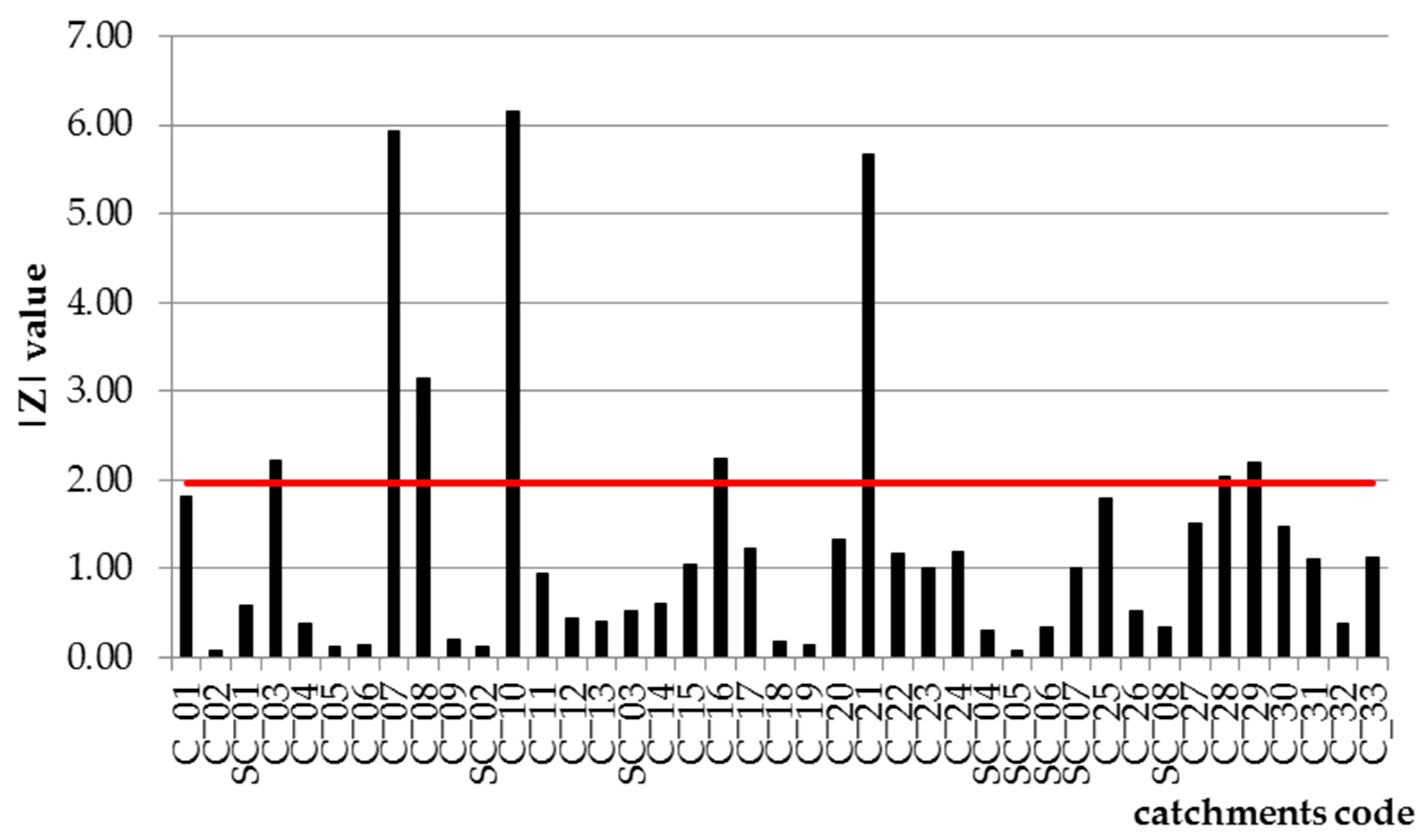
Qmax flow observation series versus the homogeneity and independence of data was carried out, using the Mann–Kendall test to examine the significance of the trend. The results of the analysis are presented in Figure 2.
Based on the obtained results, it was found that the majority of the studied rivers did not show statistically significant trends of the Qmax flows. This is evidenced by the size of normalized statistics |Z|, for which most values were lower than the critical value of this test for the significance level of α = 0.05 (Zcrit = 1.96). The following catchment areas constitute exceptions: Bystra-Kamesznica (C_03), Skawica-Zawoja (C_07), Stryszawka-Sucha (C_08), Raba-Rabka (C_10), Kirowa Woda-Kościelisko Kiry (C_16), Grajcarek-Szczawnica (C_21), San-Dwernik (C_28), and Czarny-Polana (C_29), for which the values of |Z| are bigger than Zcrit. Such results are attributed to the response of these catchments to the course of heavy rainfall of very strong intensity that occurred in Central and Eastern Europe in 1997 and 2010, causing flash floods in the upper Vistula basin [33]. In addition, as stated by Wyżga et al. [34], in recent years in the basin of the upper Vistula there had been changes in land use, which resulted in the modified occurrence of floods. For the remaining catchments, there were no statistically significant trends observed. This means that the studied variables are independent and that they derive from the same general population. Therefore, in the analysed multi-year period, no factor has appeared that would significantly affect the course of processes shaping flood flows from these catchments.
Similar research results related to the analysis of changes in the flood flows from the catchments of the upper Vistula river basin are presented in the papers [35,36], where in the majority of the studied cases there were also no statistically significant trends found in the observation series of flood flows in the upper Vistula basin. Bearing in mind that the observation series adopted for further analysis should meet the requirements of a simple random sample, the following catchments were excluded from further research: Bystra-Kamesznica, Skawica-Zawoja, Stryszawka-Sucha, Raba-Rabka, and Grajcarek-Szczawnica. On the other hand, catchments where a slight deviation from the assumed Zcrit was recorded were included in further analyses.

4.2. Estimation of the Distribution of Peak Annual Flows Using Kernel Estimates

In the present study, the estimation of the distribution of the density function in its empirical form was made for an observation series comprised of the Qmed values for the catchments, which were accepted for further analysis after the statistical verification. In the cases where the distribution showed multimodality, it was possible to conclude about the existence of many subpopulations of the examined feature. The results of calculations are presented in Figure 3.
Kernel density estimation of the Qmed flow density function, carried out for the tested catchments of the upper Vistula basin, clearly indicated the unimodal nature of the density function with the right-skewed distribution. It follows that the studied catchments located in different physiographic units of the upper Vistula river basin (Carpathian and non-Carpathian catchments) can be treated as areas with a homogeneous course of the analysed phenomenon. Hence the attempt to build a general form of a multiple regression model for determining Qmed throughout the whole area of the upper Vistula basin. However, it should be emphasized that the vast majority of the studied catchments are mountainous in nature, and therefore the course of kernel density function could be under strong pressure of flow-forming characteristics typical of catchments located in such areas. Furthermore, as stated in Santhosh and Srinivas [37], the choice of the method for estimating the smoothing parameter also has a significant impact on the result of kernel density estimation of the density function. An overly low value of the smoothing parameter may cause the estimator to exhibit multimodal features. However, at high values of this parameter, the estimator may be deprived of much information about the functional characteristics of the analysed random variable, which makes it more smooth, while indicating the unimodal distribution of this variable. According to Rutkowska et al. [38], regionalization of the catchment is based on its physiological characteristics, which have the greatest impact on the flood flows from such areas. This requires precise determination of numerical values describing these variables. In the case of using kernel estimates, it is possible to conduct an analysis only for the size of flows, without the necessity to provide any other information. A detailed analysis of the modality of kernel density function makes it possible to determine whether the given regions are homogeneous in terms of shaping the flood flows or not. For this reason, it has a certain advantage over the classical methods used for regionalization.

4.3. Determining the Form of the Equation for Calculating the Peak Flows in the Catchments of the Upper Vistula River Basin

The preliminary selection of physiographic and meteorological characteristics describing Qmed flows in the upper Vistula basin was made on the basis of the correlation matrix analysis, conducted for the initially determined values of these factors. It should be emphasized that due to the nature of statistical significance, it follows that if a significant number of determinations of correlation coefficients are performed, then statistically significant values may occur relatively frequently. There is no universal way to identify true (actual) correlations. Therefore, all results for which the strength of the correlation relationship is insufficient should be treated with caution. They should be verified in a subjective way, intuitively assessing the impact of these characteristics on the variable under study. With this in mind, final selection was made from the group of predictors (see Table 1) for the construction of the model in its final form: surface area of the catchment A, height difference in the catchment area ΔH, river network density D, arable land index Sfr, built-up index Sfu, soil imperviousness index N, and annual normal precipitation P. According to Węglarczyk [39], the number of predictors describing the dependent variable should not be overly high. This is due to the fact that each independent variable, in addition to information about the forecasted value, carries with it a certain degree of uncertainty, resulting from the observation series of this particular feature. Hence the need to determine the optimum number of independent variables, based on the quality of the model. 
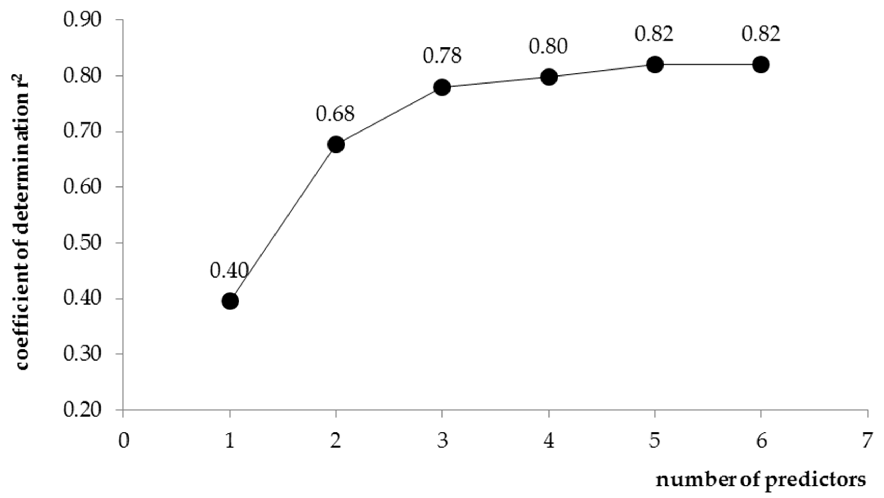
Figure 4 summarizes the values of statistics for a given number of independent variables of the analysed formula.
Based on the data presented in Figure 4, it was found that the values of the determination coefficient r2 increase significantly with the addition of further independent variables to the equation. This results from the very essence of this coefficient, as it is a non-decreasing function of the number of independent variables in multiple regression models. On the other hand, a markedly smaller increase in this characteristic was recorded after taking into account the fifth predictor in the equation. Furthermore, the addition of a sixth independent variable did not provide a significant improvement in the quality of the model. Therefore, as the final configuration of the formula for calculating the Qmed flows in the entire upper Vistula basin, a five-parameter form of the exponential equation was adopted:
Qmed = 7.388 × 10⁻⁷ × A0.755 × ΔH0.278 × D1.143 × N0.863 × P1.134 (m3·s−1)
where:
A—catchment area (km2);
ΔH—height difference in the catchment area (m a.s.l.);
D—river network density (km·km−2);
N—Boldakov’s soil imperviousness index (%);
P—annual normal precipitation in the catchment (mm).
While making the substantive verification of the established model form, it was found that it is logical. This is evidenced by the values of regression coefficients n for the predictors describing particular equations. When analysing Formula (22) in detail, it is concluded that the flow of Qmed increases with the increase of the catchment’s surface area, as well as the height difference of the catchment area, the density of the river network, the value of the soil imperviousness index, and the amount of normal annual precipitation within the catchment.
Statistical verification of the established model forms was made on the basis of the significance of the linear regression of the model, the significance of partial regression coefficients, the evaluation of redundancy between independent variables, the assumption of homoscedasticity of residuals, the lack of autocorrelation of residuals, the normality of distribution of residuals, and the evaluation of the expected value of a random component. Table 2 presents the results concerning the analysis of the significance of the linear regression of the model, and the significance of partial regression coefficients.
Based on the values summarized in Table 2, it has been found that the model form for calculating Qmed in the entire upper Vistula basin is characterized by a statistically significant value of the F statistic, for which the p-value is less than the assumed significance level of α = 0.05. In turn, statistically significant values of pi partial regression coefficients occur for the catchment area and river network density. Bearing in mind the analysis regarding the determination of the optimum number of predictors in the equations, it was decided that statistically insignificant parameters should be retained, because their removal decreases the quality of the examined models, reflected by a marked decrease in the value of the determination coefficient r2.
The evaluation of the redundancy of variables is based on the so-called tolerance factor. In cases when the value of that factor was higher than 0.1, it was concluded that there is no collinearity of independent variables. The results of this analysis are summarized in Table 3.
When analysing the values listed in Table 3, it was found that the tolerance for all variables is high (above 0.1). In addition, the values of coefficient r2c differ significantly from one. Thus, independent variables do not show redundancy in regression equations, which indicates the lack of their collinearity. Furthermore, the relatively high values of semi-partial correlations in the studied equation forms, for independent variables, indicate relatively high correlations with the dependent variable.
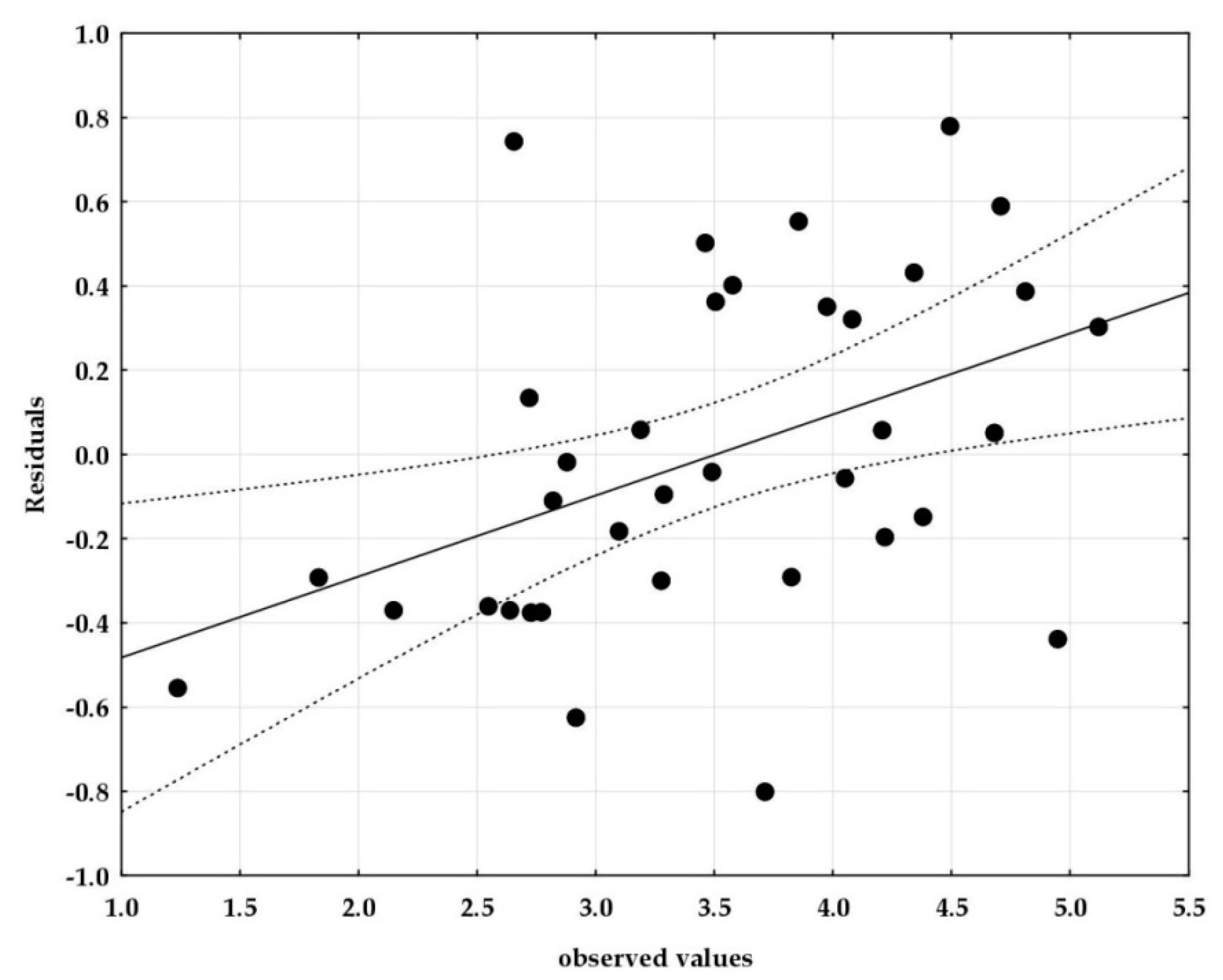
The assumption of constancy of the variance of the random component for individual values of independent variables (homoscedasticity) was verified using the scatter plots. Figure 5 is a graph of predicted values relative to residual values.
When analysing the values summarized in Figure 5, we noted the lack of heteroscedasticity (violation of the assumption of homoscedasticity) of the random variables being analysed. Points on the graph are arranged in the form of an evenly distributed cloud, and there are no clear systems of the points that form individual groups. Therefore, there is no reason to reject the assumption of constancy of the random component variance, for individual independent variables.
To verify the autocorrelation of the residuals of the models, the Durbin-Watson statistics were used. The results of the analysis are summarized in Table 4. Based on the results as seen in Table 4, the hypothesis was adopted that the random elements were not correlated.
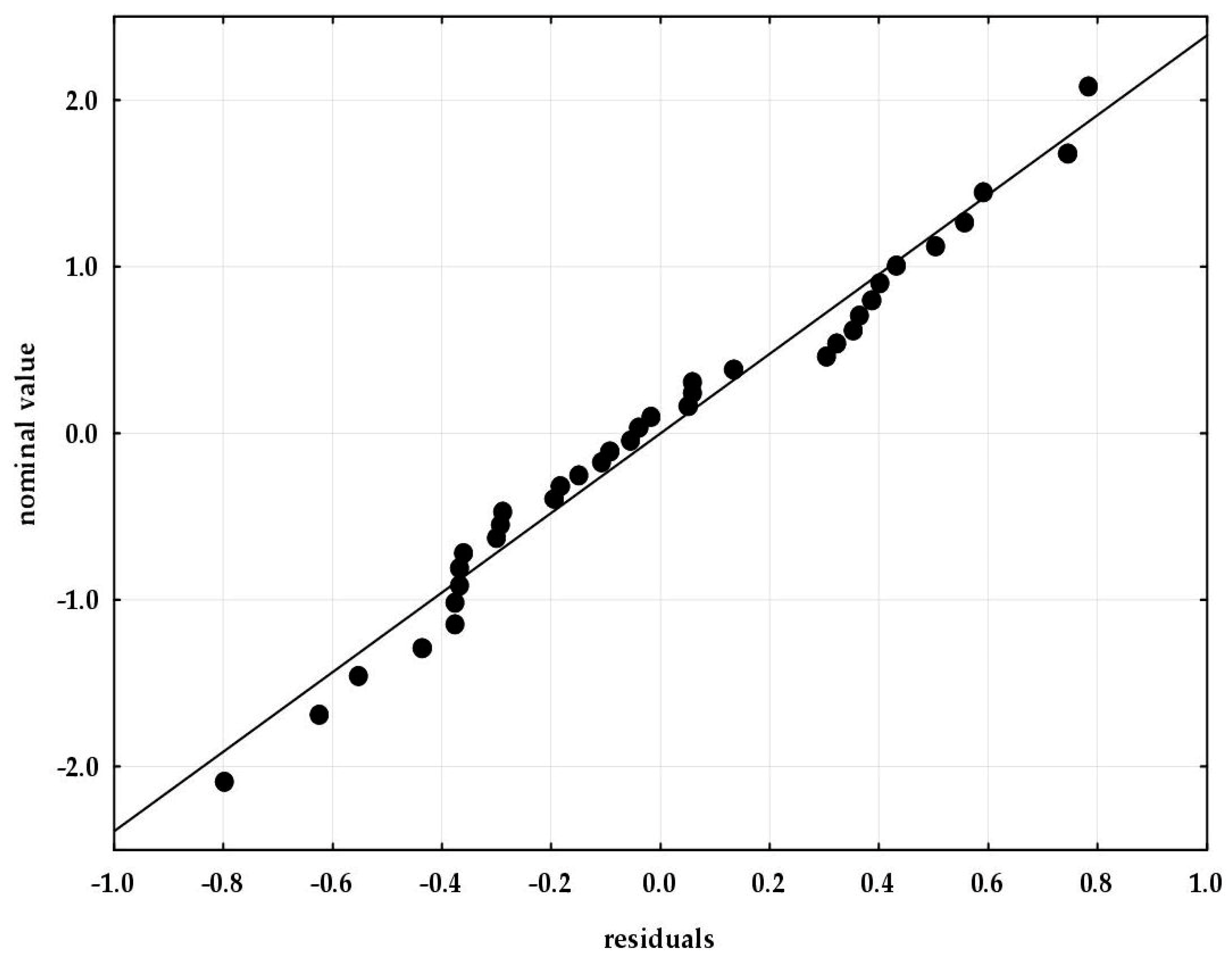
The normality of the distribution of residues was verified using the normality plot. Figure 6 presents a chart of nominal (expected) values relative to residual values obtained by applying the tested form of the empirical model. Based on the normality plot of the residuals, it was found that for the analysed equation, most points are arranged along a straight line. Hence the inference that in these cases the distribution of residues is consistent with the normal distribution.
The verification of the assumption about the zero value of the expected random component εi was made based on the analysis of average residuals for the studied forms of equations. The results are summarized in Table 5.
Based on the results summarized in Table 5, it was found that the average values of the residuals for the developed model are 0; therefore, the hypothesis with a zero value for the random component εi is true. This means that the distortions (random components) do not show any tendency of the empirical values of the dependent variable deviating from the theoretical values in any direction (either plus or minus).
Verification of the determined correlation for the forecast of Qmed flows in the catchments of the upper Vistula basin was made on the basis of independent hydrometric material for the following catchments: Przemsza-Piwoń, Skawinka-Radziszów (non-Carpathian catchments) and Stradomka-Stradomka, Niedziczanka-Niedzica, Jasiołka-Zboiska (Carpathian catchments). Additionally, the confidence interval was estimated by applying the Formulas (6) and (7), for the significance level of α = 0.05. The results are shown in Table 6.
Based on the results summarized in Table 6, it was found that the obtained form of the empirical model produces satisfying results. This is evidenced by the small differences between Qmed and Q med p . Therefore, it is recommended that Formula (22) be used in the ungauged basins of the upper Vistula river basin. This will eliminate the problem related to the choice of the appropriate regional equation if the river flows through several physiographic regions, and above all, through both Carpathians and non-Carpathian areas. Such rivers may demonstrate characteristics acquired in the upper course, even though their water gauge profile is far beyond the region’s reach. Regarding the analysis we have conducted, concerning the determination of the lower and upper boundaries of the confidence interval for the determined form of the empirical model, it can be stated that for the confidence level of 95%, the predicted Qmed values remain within the range described by Equation (6).

4.4. Determination of Dimensionless Quantiles’ Values for the Calculation of Peak Annual Flows with a Defined Frequency of Occurrence

Determination of the values of dimensionless μT quantiles was meant to facilitate the determination of QT flows, based on Formula (22). To determine the quantile values of μT, firstly, the best-fit probability distribution function to calculate the QT was indicated. Then the statistical distributions recommended in Poland were subjected to analysis: Pearson type III (PIII), Weibull, and log-normal.
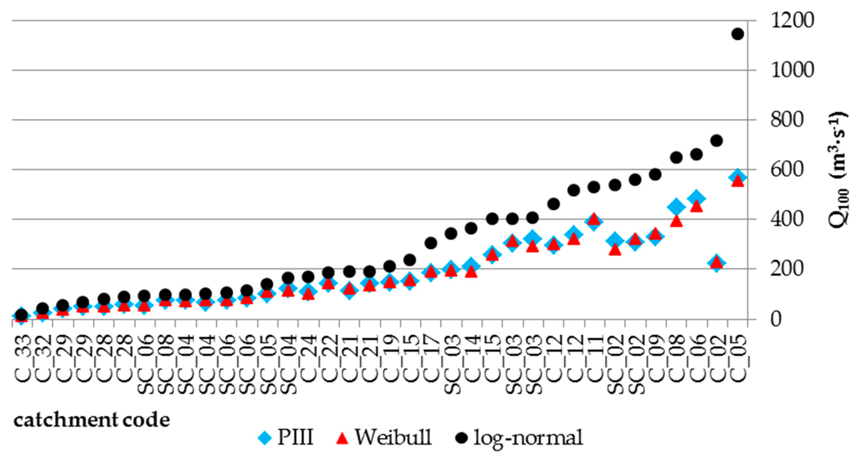
 Figure 7 presents Q100 values determined by the studied probability distributions.
Based on the results summarized in Figure 7, it was found that the highest Q100 values were obtained by means of the log-normal distribution. However, for the Pearson distribution type III and for the Weibull distribution, these values remained at similar levels. Obtaining the highest Q100 quantile values using the log-normal function is justified by the properties of this particular model. The log-normal function is fat-tailed to the right, which means that with the same row of the upper quantile, e.g., p ≤ 0.2, it generates much higher quantile values compared to other probability distributions [14]. Furthermore, the effects of the flood regime may also influence such results. The peak flows are rare (occurring once a year). However, their values are significant, and they stand out clearly from other data. Therefore, fat-tailed distributions can effectively describe empirical sequences of such variables.
The selection of the theoretical function best fitting the empirical distribution of the Qmax variable was made using the Akaike’s information criterion (AIC) ranking method. The results of the calculations are summarized in Table 7.
Based on the results summarized in Table 7, it was found that in a majority of cases (58% of all the studied catchments) the log-normal distribution best approximates the empirical Qmax sequences. However, for the Pearson distribution type III and for the Weibull distribution, the best fit was obtained in 9 and in 6 research catchments, respectively. Bearing in mind the obtained results and the sum of ranks, log-normal was adopted as the recommended statistical distribution for estimating QT quantiles in the upper Vistula basin. Kuczera obtained similar results, as quoted in his paper [40], where the author pointed out that the best theoretical distribution for the approximation of Qmax flows is the log-normal distribution. Strupczewski et al. [41] also found that the log-normal distribution best describes the empirical distributions of the analysed random variables.
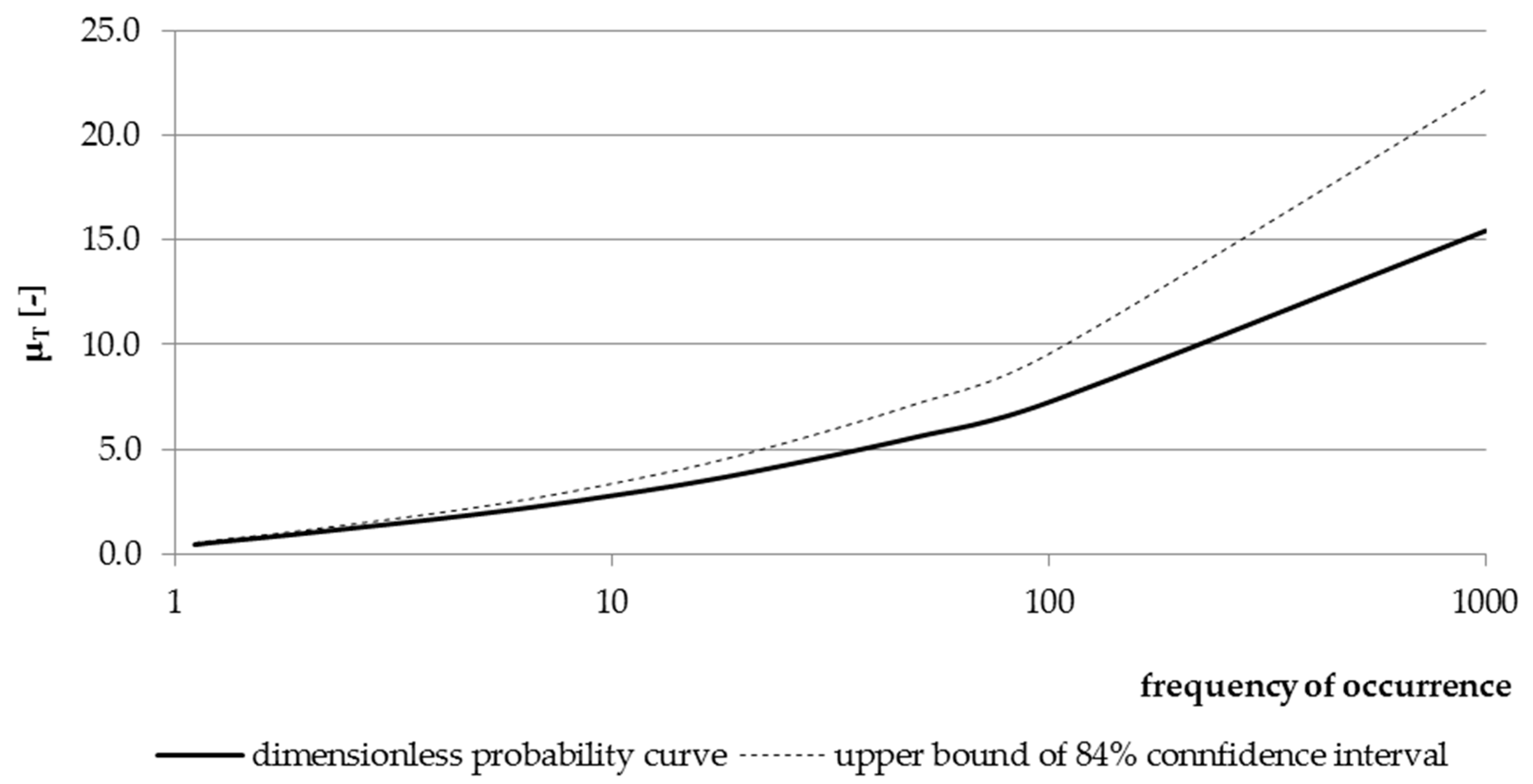
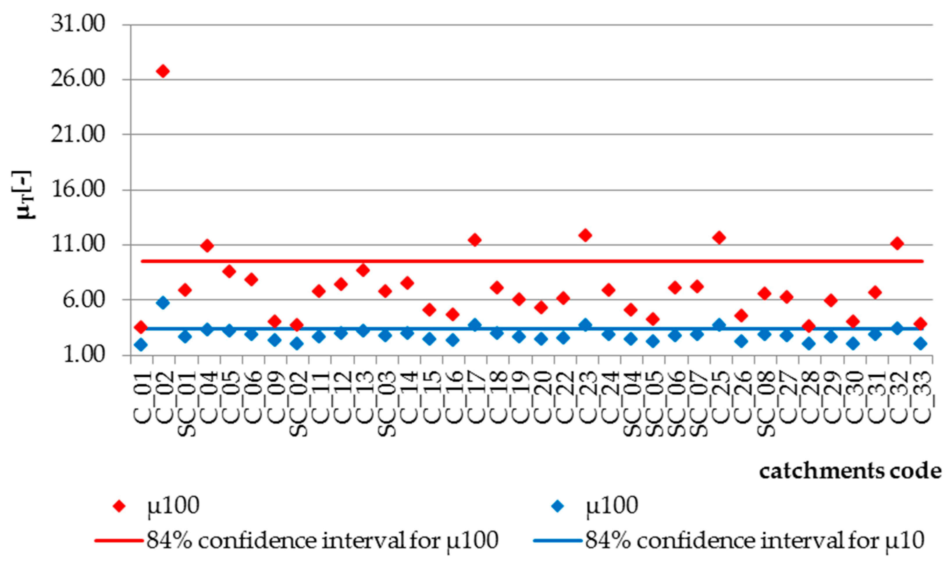
Based on the recommended statistical distribution, a non-dimensional probability curve was determined (see Figure 8). The curve was verified based on the results summarized in Figure 9. Verification of the non-dimensional probability curve, subject to log-normal distribution, produced satisfactory results. In the total number of 36 tested catchments of the entire upper Vistula basin, the Q10/Qmed quantile was outside the upper boundary of the confidence interval 4 times (11%), and the Q100/Qmed quantile, 6 times (17%). According to the definition of the upper boundary at 84% of the confidence interval, for 36 cases outside this limit, there may be 5 observations (16% of 36 cases). With a small number of observations, such a result can be considered acceptable. Therefore, the log-normal distribution was assumed as the basis for determining QT quantiles using the determined empirical correlation.
Bearing in mind the calculations we have carried out, the final form of the empirical model for estimating QT flows in the catchments of the ungauged upper Vistula basin was obtained as follows:
QT = Qmed × μT (m3·s−1)
where:
Qmed—median annual flow, determined by Formula (22) (m3·s−1);
μT—dimensionless value of distribution quantile for the assumed frequency of occurrence, taken from Figure 8 (-).
Thus, the developed empirical formula is recommended for use in catchments whose surface areas range from 50 to 600 km2.
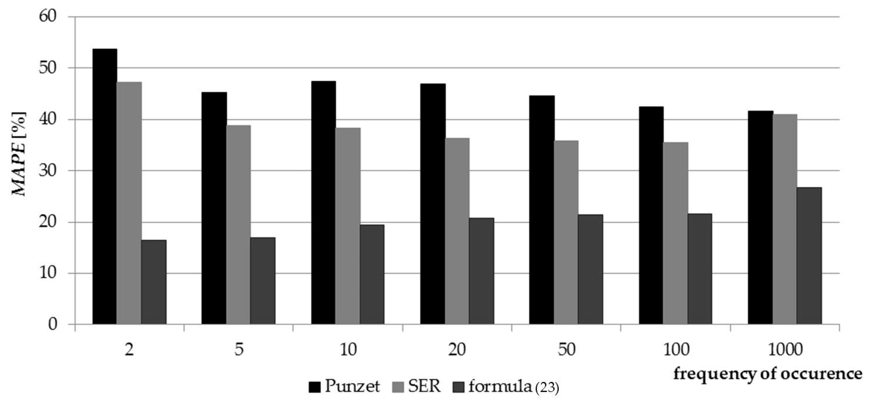
As a complement to the conducted research, verification of the established formula (23) for estimating QT quantiles was performed against the currently used empirical formulas in the upper Vistula basin: Punzet’s and the spatial equation of regression (SER). The results of the verification are presented in Figure 10. Based on the obtained results, it was found that compared to the Punzet and SER formula, the values obtained with Formula (23) present the lowest MAPE value for each QT quantile. Standard error of estimating QT using the Punzet formula is 46%; when using the area regression equation, it is 39%, and when using formula (23) it is 21%. Therefore, it is concluded that the developed equation can be a viable alternative to the currently used empirical formulas for calculating QT in ungauged catchments of the upper Vistula basin.

5. Conclusions

The aim of the work was to determine the form of a new empirical model for estimating quantiles of peak annual flows with a defined frequency of occurrence in ungauged catchments of the upper Vistula basin. Based on the research we conducted, it was found that in the majority of the catchments there are no statistically significant trends of peak annual flows. This is evidenced by the results of the analysis carried out with the application of the Mann–Kendall test, confirming the invariability of hydrological conditions and the stationarity of the characteristics affecting the volume of flood flows (values of Z statistics from the Mann–Kendall test for the analysed time series below 1.96). Kernel estimation of the distribution function of median flows in the upper Vistula basin clearly indicated the unimodal character of the empirical distribution function, which may indicate homogeneous conditions affecting the flood flows in the analysed multi-year period, in all of the studied catchments. Since the application of this method requires knowledge of only the factor for which calculations are made; hence, it may compete with other commonly used methods of regionalization. Based on the computations conducted in the study, it was demonstrated that the course of floods in the upper Vistula basin is most influenced by such factors as: surface area of the catchment, height difference in the catchment area, river network density, imperviousness of the soil, and normal annual precipitation. Based on the results obtained using the AIC criterion, it was found that among the probability distribution types tested for QT calculation in the upper Vistula basin, the empirical Qmax sequences were approximated best by the log-normal distribution. Verification of the established correlation for QT estimation in the upper Vistula basin showed that the formula functions properly, as evidenced by the MAPE values (standard error of QT estimating was 21% while for currently used empirical formulas in upper Vistula basin: Punzet and SER it was 46 and 39% respectively). The determined form of the empirical equation finds application in the entire upper Vistula basin, for the catchments with a surface area of 50 to 600 km2.

Author Contributions

Conceptualization, D.M., A.W.; methodology, D.M., A.W.; software, D.M., T.S.; validation, D.M., A.W.; formal analysis, D.M.; investigation, D.M., A.W.; resources, D.M., A.W.; data curation, D.M.; writing—original draft preparation, D.M.; writing—review and editing, D.M., A.W., T.S., G.K.; visualization, D.M., T.S., G.K.; supervision, A.W.

Funding

This research received no external funding.

Acknowledgments

The results are part of the Phd thesis: Impact of physiographic and meteorological factors on peak annual flows with set return period formation in the catchments of upper Vistula basin. This research was financed by Ministry of Science and Higher Education of the Republic of Poland.

Conflicts of Interest

The authors declare no conflict of interest.

References

  1. Li, T.; Guo, S.; Chen, L.; Guo, J. Bivariate flood frequency analysis with historical information based on copula. J. Hydrol. Eng. 2013, 18, 1018–1030. [Google Scholar] [CrossRef]
  2. Młyński, D.; Petroselli, A.; Wałęga, A. Flood frequency analysis by an event-based rainfall-runoff model in selected catchments of southern Poland. Soil Water Res. 2018, 13, 170–176. [Google Scholar] [Green Version]
  3. Bezak, N.; Brillyc, M.; Šraj, M. Flood frequency analyses, statistical trends and seasonality analyses of discharge data: A case study of the Litija station on the Sava River. J. Flood Risk Manag. 2016, 9, 154–156. [Google Scholar] [CrossRef]
  4. Bhagat, N. Flood frequency analysis using Gumbel’s distribution method: A case study of lower Mahi basin, India. J. Water Resour. Ocean Sci. 2017, 6, 51–54. [Google Scholar] [CrossRef]
  5. Abdulrazzak, M.; Elfeki, A.; Kamis, A.S.; Kassab, M.; Alamri, N.; Noor, K.; Chaabani, A. The impact of rainfall distribution patterns on hydrological and hydraulic response in arid regions: Case study Medina, Saudi Arabia. Arab. J. Geosci. 2018, 11, 679–697. [Google Scholar] [CrossRef]
  6. Machado, M.J.; Boterom, B.A.; López, J.; Francés, F.; Díez-Herrero, A.; Benito, G. Flood frequency analysis of historical flood data under stationary and non-stationary modeling. Hydrol. Earth Syst. Sci. 2015, 19, 2561–2576. [Google Scholar] [CrossRef]
  7. Ahn, K.H.; Palmer, R. Regional flood frequency analysis using spatial proximity and basin characteristics: Quantile regression vs. parameter regression technique. J. Hydrol. 2016, 540, 515–526. [Google Scholar] [CrossRef]
  8. Nyeko-Ogiramoi, P.; Willems, P.; Mutua, F.; Moges, S.A. An elusive search for regional flood frequency estimates in the River Nile basin. Hydrol. Earth Syst. Sci. 2012, 16, 3149–3163. [Google Scholar] [CrossRef] [Green Version]
  9. Haddad, K.; Rahman, A.; Stedinger, J.R. Regional flood frequency analysis using Bayesian generalized least squares: A comparison between quantile and parameter regression techniques. Hydrol. Process. 2012, 26, 1008–1021. [Google Scholar] [CrossRef]
  10. Haddad, K.; Rahman, A. Regional flood frequency analysis in eastern Australia: Bayesian GLS regression-based methods within fixed region and ROI framework—Quantile regression vs. parameter regression technique. J. Hydrol. 2012, 430, 142–161. [Google Scholar] [CrossRef]
  11. Alam, J.; Muzzammil, M.; Khan, M.K. Regional flood frequency analysis: Comparison of L-moment and conventional approaches for an Indian catchment. ISH J. Hydraul. Eng. 2016, 22, 247–253. [Google Scholar] [CrossRef]
  12. Cupak, A.; Wałęga, A.; Michalec, B. Cluster analysis in determination of hydrologically homogeneous regions with low flow. Acta Sci. Pol. Form. Circumiectus 2017, 16, 53–56. [Google Scholar] [CrossRef]
  13. Cupak, A. Initial results of nonhierarchical cluster methods use for fow flow grouping. J. Ecol. Eng. 2017, 18, 44–50. [Google Scholar] [CrossRef]
  14. Kochanek, K.; Feluch, W. The estimation of flood quantiles of the selected heavy-tailed distributions by means of the method of generalised moments. Prz. Geofiz. 2016, 3–4, 171–193. (In Polish) [Google Scholar]
  15. Hirabayashi, Y.; Mahendran, R.; Koirala, S.; Konoshima, L.; Yamazaki, D.; Watanabe, S.; Kim, H.; Kanae, S. Global flood risk under climate change. Nat. Clim. Chang. 2013, 3, 816–821. [Google Scholar] [CrossRef]
  16. Qin, X.S.; Lu, Y. Study of climate change impact on flood frequencies: A combined weather generator and hydrological modeling approach. J. Hydrometeorol. 2014, 3, 1205–1219. [Google Scholar] [CrossRef]
  17. Kundzewicz, Z.W.; Pińskwar, I.; Choryński, A.; Wyżga, B. Floods still pose a hazard. Aura 2017, 3, 3–8. (In Polish) [Google Scholar]
  18. Kundzewicz, Z.W.; Stoffel, M.; Niedźwiedź, T.; Wyżga, B. Flood Risk in the Upper Vistula Basin; Springer: Basel, Switzerland, 2016. [Google Scholar]
  19. Młyński, D.; Cebulska, M.; Wałęga, A. Trends, variability, and seasonality of Maximum annual daily precipitation in the upper Vistula basin, Poland. Atmosphere 2018, 9, 313. [Google Scholar] [CrossRef]
  20. Jeneiová, K.; Kohnová, S.; Sabo, M. Detecting trends in the annual maximum discharges in the Vah River Basin, Slovakia. Acta Silvatica et Lignaria Hungarica 2014, 10, 133–144. [Google Scholar] [CrossRef]
  21. Zhang, Y.; Wang, J. K-nearest neighbors and a kernel density estimator for GEFCom2014 probabilistic wind power forecasting. Int. J. Forecast. 2016, 32, 1074–1080. [Google Scholar] [CrossRef]
  22. Silverman, B.W. Density Estimation for Statistics and Data Analysis; Chapman & Hall: London, UK, 1986. [Google Scholar]
  23. Scailet, O. Density estimation using inverse and reciprocal inverse Gaussian kernels. J. Nonparametr. Stat. 2004, 16, 217–226. [Google Scholar] [CrossRef] [Green Version]
  24. Murphy, C.; Cunnane, C.; Das, S.; Mandal, U. Flood Frequency Estimation; Technical Research Reports; NNUI Galway: Galway, Ireland; NUI Maynnooth: Maynnooth, Ireland, 2014. [Google Scholar]
  25. Choubin, B.; Khalighi-Sigaroodi, S.; Malekian, A.; Kişi, Ö. Multiple linear regression, multi-layer perceptron network and adaptive neuro-fuzzy inference system for forecasting precipitation based on large-scale climate signals. Hydrol. Sci. J. 2016, 61, 1001–1009. [Google Scholar] [CrossRef]
  26. Keith, T.Z. Multiple Regression and Beyond; Routledge: New York, NY, USA, 2019. [Google Scholar]
  27. Młyński, D. Analysis of the form of probability distribution to calculate flood frequency in selected mountain river. Episteme 2016, 30, 399–412. (In Polish) [Google Scholar]
  28. Kim, H.; Kim, S.; Shin, H.; Heo, J. Appropriate model selection methods for nonstationary generalized extreme value models. J. Hydrol. 2017, 547, 557–574. [Google Scholar] [CrossRef]
  29. Stachý, J.; Fal, B. The principles of the probable floods evaluation. Prace Instytutu Badawczego Dróg i Mostów 1986, 3–4, 92–149. (In Polish) [Google Scholar]
  30. Młyński, D.; Wałęga, A.; Petroselli, A. Verification of empirical formulas for calculating annual peak flows witch specific return period in the upper Vistula basin. Acta Sci. Pol. Form. Circumeticus 2018, 17, 145–154. [Google Scholar] [CrossRef]
  31. Adewumi, A.A.; Owolabi, T.O.; Alde, I.O.; Olatunji, S.O. Estimation of physical, mechanical and hydrological properties of permeable concrete using computational intelligence approach. Appl. Soft Comput. 2016, 42, 342–350. [Google Scholar] [CrossRef]
  32. Kim, S.; Kim, H. A new metric of absolute percentage error for intermittent demand forecast. Int. J. Forecast. 2016, 32, 669–679. [Google Scholar] [CrossRef]
  33. Młyński, D.; Wałęga, A.; Petroselli, A.; Tauro, F.; Cebulska, M. Estimating Maximum Daily Precipitation in the Upper Vistula Basin, Poland. Atmosphere 2019, 10, 43. [Google Scholar] [CrossRef]
  34. Wyżga, B.; Kundzewicz, Z.W.; Ruiz-Villanueva, V.; Zawiejska, J. Flood generation mechanisms and changes in principal drivers. In Flood Risk in the Upper Vistula Basin; Kundzewicz, Z., Stoffel, M., Niedźwiedź, T., Wyżga, B., Eds.; Springer: Cham, Switzerland, 2016. [Google Scholar]
  35. Walega, A.; Młyński, D.; Bogdał, A.; Kowalik, T. Analysis of the course and frequency of high water stages in selected catchments of the upper Vistula basin in the south of Poland. Water 2016, 8, 394. [Google Scholar] [CrossRef]
  36. Kundzewicz, Z.W.; Stoffel, M.; Kaczka, R.J.; Wyżga, B.; Niedźwiedź, T.; Pińskwar, I.; Ruiz-Villanueva, V.; Łupikasza, E.; Czajka, B.; Ballesteros-Canovas, J.A.; et al. Floods at the northern foothills of the Tatra mountains—A Polish-Swiss research project. Acta Geophys. 2014, 62, 620–641. [Google Scholar] [CrossRef]
  37. Santhosh, D.; Srinivas, V. Bivariate frequency analysis of floods using a diffusion based kernel density estimator. Water Resour. Res. 2013, 49, 8328–8343. [Google Scholar] [CrossRef]
  38. Rutkowska, A.; Żelazny, M.; Kohnová, S.; Łyp, M.; Banasik, K. Regional l-moment-based flood frequency analysis in the upper Vistula river basin, Poland. Pure Appl. Geophys. 2017, 174, 701–721. [Google Scholar] [CrossRef]
  39. Węglarczyk, S. Eight reasons to revise the formulas used in calculation of the maximum annual flows with a set exceedance probability in Poland. Gospodarka Wodna 2015, 11, 323–328. (In Polish) [Google Scholar]
  40. Kuczera, G. Robust flood frequency models. Water Resour. Res. 1982, 18, 315–324. [Google Scholar] [CrossRef]
  41. Strupczewski, W.G.; Singh, V.P.; Mitosek, H.T. Non-stationary approach to at site flood frequency modeling. III. Flood analysis for Polish rivers. J. Hydrol. 2001, 248, 152–167. [Google Scholar] [CrossRef]
Figure 1. Location of studied catchment areas in upper Vistula basin, set against digital elevation model.
Water 11 00601 g001
Figure 2. Results of the Mann–Kendall test of trend significance for the studied catchments.
Water 11 00601 g002
Figure 3. The course of the estimated kernel density function of Qmed flows for the studied catchments of the upper Vistula basin.
Water 11 00601 g003
Figure 4. Impact of the number of predictors on the value of the coefficient of determination for the analysed form of the model for estimating Qmed throughout the upper Vistula basin.
Water 11 00601 g004
Figure 5. Diagram of the predicted values versus residual values for the model for estimating Qmed in the upper Vistula basin.
Water 11 00601 g005
Figure 6. Diagram of normal distribution of residuals for the model for estimating Qmed in the upper Vistula basin.
Water 11 00601 g006
Figure 7. Values of Q100 for the studied catchments, determined using the analyses statistical distributions.
Water 11 00601 g007
Figure 8. Dimensionless probability curve of annual peak flows for the catchments of upper Vistula river basin.
Water 11 00601 g008
Figure 9. Verification of the dimensionless probability curve for the upper Vistula river basin.
Water 11 00601 g009
Figure 10. MAPE values for the estimation of QT quantiles for the analysed empirical formulae.
Water 11 00601 g010
Table 1. Physiographic and meteorological characteristics of the catchment applicable to the construction of the empirical Qmed model.
Type of the CharacteristicsCharacteristicsSymbolUnit
geometricMaximum length of the catchmentLmaxkm
Surface area of the catchmentAkm2
Catchment circumference O in kmOkm
Average width of the catchmentBxkm
morphometricMinimum heightHminm a.s.l.
Average heightHavem a.s.l.
Maximum heightHmaxm a.s.l.
Height differences in the catchmentΔHm a.s.l.
Average slope in the catchmentJ-
hydrographic network-relatedLength of the main watercourseLkm
Length of the dry valleylkm
Slope of the watercourseI-
Density of the river networkDkm/km2
related to land use in the catchmentForest coverage indexSfl-
Agricultural area indexSfr-
Built-up indexSfu-
lithologicalSoil imperviousness indexN%
meteorologicalNormal annual rainfallPmm
Table 2. Results of the significance analysis of linear regression model, and the significance of the component coefficients of regression for the model for estimating Qmed throughout the upper Vistula basin.
VariableFpn*Standard Error of n*nStandard Error of btpi
a25.1610.000 −14.1184.301−3.2830.003
A0.7590.1030.7550.1027.3950.000
ΔH0.1810.1490.2780.2291.2140.234
D0.5000.1311.1430.2993.8230.001
N0.1930.1190.8630.5311.6250.115
Pn0.3030.1591.1340.5941.9080.066
F—Fisher-Snedecor distribution; pp value for the regression model; a—value of the absolute term; n*—normalised coefficient of regression; n—coefficient of regression; t—quotient b/(standard effort of b); pip value for partial coefficients of regression models.
Table 3. Results of the collinearity analysis of independent variables in the studied forms of the model for determining Qmed in the upper Vistula basin.
VariableTolerancer2cPartial CorrelationSemi-Partial Correlation
A0.6100.3900.8040.592
ΔH0.2880.7120.2160.097
D0.3750.6250.5720.306
N0.4550.5450.2840.130
P0.2540.7460.3290.153
r2c—value of the coefficient of determination between the given variable and all other independent variables.
Table 4. Results of the autocorrelation analysis of residuals, conducted using Durbin-Watson test (source: own study).
NkdldgD
3651.181.802.321
N—number of cases; k—number of variables in the equation; dl, dg—threshold values of the Durbin-Watson statistic; D—Durbin-Watson statistic.
Table 5. Analysis of outlier residuals for the studied forms of the models for estimating Qmed in the upper Vistula basin.
Residuals εi
minimum−0.802
maximum0.780
average (mean)0.000
median−0.050
Table 6. Values Qmed and confidence intervals for the values obtained from the adopted empirical model.
River-ProfileQmed (m3·s−1) Q med p ( m 3 · s 1 ) Lower Boundary of Confidence Interval (m3·s−1)Upper Boundary of Confidence Interval (m3·s−1)
Przemsza-Piwoń14.809.155.0016.61
Skawinka-Skawina67.4065.9150.9184.77
Stradomka-Stradomka87.6063.8347.4984.77
Niedziczanka-Niedzica42.8035.2426.3139.25
Jasiołka-Zboiska58.7061.1244.2683.93
Qmed—median of annual peak flows, determined on the basis of the observation series; Q med p —flow calculated according to Formula (22).
Table 7. Ranks of statistical distributions used for estimating QT in the studied catchments within the upper Vistula basin (source: own study).
DistributionRank
123Σ of ranks
PIII924366
W6121884
L-N2111465

