Article

Mapping Riparian Vegetation Functions Using 3D Bispectral LiDAR Data

UMR 6554 LETG Rennes, Place du Recteur Henri le Moal, CS 24037, 35043 Rennes CEDEX, France
*
Author to whom correspondence should be addressed.
Water 2019, 11(3), 483; https://doi.org/10.3390/w11030483
Submission received: 11 February 2019 / Revised: 25 February 2019 / Accepted: 28 February 2019 / Published: 7 March 2019
(This article belongs to the Special Issue Riparian Vegetation in River Functioning)

Abstract

:
Riparian zones experience many anthropic pressures and are the subject of European legislation to encourage their monitoring and management, to attenuate these pressures. Assessing the effectiveness of management practices requires producing indicators of ecological functions. Laser Detection and Ranging (LiDAR) data can provide valuable information to assess the ecological status of riparian zones. The objective of this study was to evaluate the potential of LiDAR point clouds to produce indicators of riparian zone status. We used 3D bispectral LiDAR data to produce several indicators of a riparian zone of a dammed river in Normandy (France). The indicators were produced either directly from the 3D point clouds (e.g., biomass overhanging the channel, variation in canopy height) or indirectly, by applying the Random Forest classification algorithm to the point clouds. Results highlight the potential of 3D LiDAR point clouds to produce indicators with sufficient accuracy (ca. 80% for the number of trunks and 68% for species composition). Our results also reveal advantages of using metrics related to the internal structure of trees, such as penetration indexes. However, intensity metrics calculated using bispectral properties of LiDAR did not improve the quality of classifications. Longitudinal analysis of the indicators revealed a difference in attributes between the reservoir and areas downstream from it.

1. Introduction

Riparian zones provide multiple ecosystem services, such as sediment bank stabilization, water flux regulation, flood prevention, and habitat provision [1]. The riparian zone describes the area that interacts with the river, i.e., that can be flooded by the river and can provide materials to the river. Since riparian zones intersect land and water, they are exceptionally rich in biodiversity [2]. They function as ecological corridors and provide a high diversity of habitats for birds and other animal species [3]. However, riparian zones are subject to many anthropic pressures, such as land cover modification (urbanization, deforestation, etc.) and flow regulation. For example, in Europe, 90% of riparian zones have disappeared or are degraded [4]. As a consequence, river ecosystems are the focus of management and restoration projects [5].
The effectiveness of river management and restoration projects is insufficiently monitored [6], in part due to the difficulty in producing indicators that can assess the effectiveness of management practices. Indicators can be defined as a metric or a combination of metrics to assess the status or a change in status. These indicators form the foundation of an assessment [7]. However, producing indicators can be difficult for river systems. This is particularly true for riparian vegetation. The linear shape and structural complexity of riparian vegetation may limit the production of indicators for monitoring and raising several methodological issues [8]. To be effective, monitoring indicators need to have certain characteristics and must be meaningful for the processes considered; simple to produce and understandable to managers, spatialized at the scale of the entire river (large scale), produced quickly (e.g., immediately after a flood or dam removal) and, produced with high temporal frequency (to finely assess the river’s response to management practices) [5]. These indicators must be produced before management practices occur, to document the initial state of the system, and after they occur, to monitor their effects. The indicators produced need to correspond with the objectives of management or restoration [9]. This requires producing a wide range of indicators related to all functions that riparian vegetation provide.
Remote sensing is a tool increasingly used to map the status of ecosystems. Over the past decade, a large body of research has focused on building this framework, and several studies used remote sensing data to produce precise maps of riparian zone attributes [10,11,12,13,14,15]. Since many riparian functions are related to the three dimensional (3D) structure of vegetation, indicators reflecting the latter have been produced using the new generation of remote sensing data, such as that from Airborne Laser Scanning (ALS) or Laser Detection and Ranging (LiDAR). Doing so remains challenging, however, due to the complexity of riparian zones (i.e., high species biodiversity, stratification, and variability in the size of riparian patches) Better methodological frameworks are thus required to map 3D riparian vegetation characteristics at a large scale [8].
Laser scanning consists of sending laser pulses from an aircraft-mounted laser and recording the information acquired each time the pulse touches a surface. Since the laser pulse is narrow (a few cm), it can penetrate surfaces such as tree canopies and return 3D information. Therefore, LiDAR data are widely used in forestry to estimate forest inventory components such as tree species [16], aboveground biomass [17,18], diameter at breast height (DBH) [19], and stem density. Most of these studies focused on non-riparian forests, especially large coniferous forests [16]. Riparian vegetation differs from these forests, usually having high structural complexity due to high species richness and vertical stratification [16].
Only a few studies have focused on riparian attributes and LiDAR data [20], and most of them used only 2D products of LiDAR data, such as digital elevation models (DEM) and canopy height models (CHM). For example, Akasaka, et al. [10,15,21] used CHM to characterize the variance in canopy height. Riedler, et al. [15] used CHM to count the number of old trees, assuming that taller and larger trees were older. Akasaka, et al. [10] measured the volume of open area under the tree canopy using stream width, height from the water surface to the lowest tree, and longitudinal distance from upstream to downstream (20 m). Antonarakis, et al. [11] used LiDAR data to estimate the vegetative fluid resistance of large riparian stems. They were able to extract tree crowns using a CHM. Straatsma, et al. [22] used LiDAR data to map vegetation roughness. These studies did not take full advantage of all LiDAR data information, especially stratification and spectral information. Using only the highest (top of the canopy) and lowest (ground) returns of LiDAR data, they ignored the information between these points.
In addition to elevation information, LiDAR data provide information about the intensity of energy absorbed by the objects in the wavelength of the laser. LiDAR usually records intensity information in the near-infrared (NIR) channel because it penetrates canopies the most [16]. Intensity is related to the spectral properties of objects, such as chlorophyll content for vegetation, but is also strongly influenced by other parameters, such as scan angle and flight altitude, which can make analyzing this information difficult. The new generation of LiDAR can record information in multiple wavelengths simultaneously, which allows one to normalize the intensity and cancel the bias due to scan angle and flight altitude. Since this type of LiDAR is relatively new, few studies have focused on the advantages of using two or more channels in LiDAR studies [23,24], and no studies have focused on structurally complex riparian buffers.
Consequently, the objectives of this study were (1) to develop spatialized indicators of riparian functions using 3D bispectral LiDAR data and (2) to test the effect of LiDAR intensity on the accuracy of the indicators. Hence, we mapped species composition, herbaceous stratum density, and shrub stratum density, number of trunks per tree, canopy stratification, and the area and biomass of leaves overhanging the channel.

2. Materials and Methods

2.1. Study Site

The study was conducted along the Sélune River, France (Figure 1). The Sélune River flows 91 km from Saint-Cyr-du-Bailleul to the Mont-Saint-Michel Bay in Normandy. The climate is oceanic, with precipitation throughout the year. The growing season runs from April–August. The Sélune watershed covers 1009 km2 and is predominantly agricultural. Two dams are located on the Sélune River—Vezins and La Roche-qui-Boit—that form a 19 km-long reservoir. Both will be removed by the French Government in 2020 to restore river connectivity and because they no longer produce electricity profitably. Riparian zones along the Sélune River take three forms: narrow buffer strips, floodplain forest, and hillslope forest (in the reservoir). Tree lines (80% of riparian trees along the Sélune River) are located upstream and downstream of the reservoir.
All trees in the riparian zone were considered (Figure 1). The riparian zone was composed of the floodplain (extracted from the DEM according to the Alber and Piégay [25] method), a floodplain forest, buffer strips, and a hillslope forest (an arbitrary 30 m wide buffer along the river).

2.2. General Framework

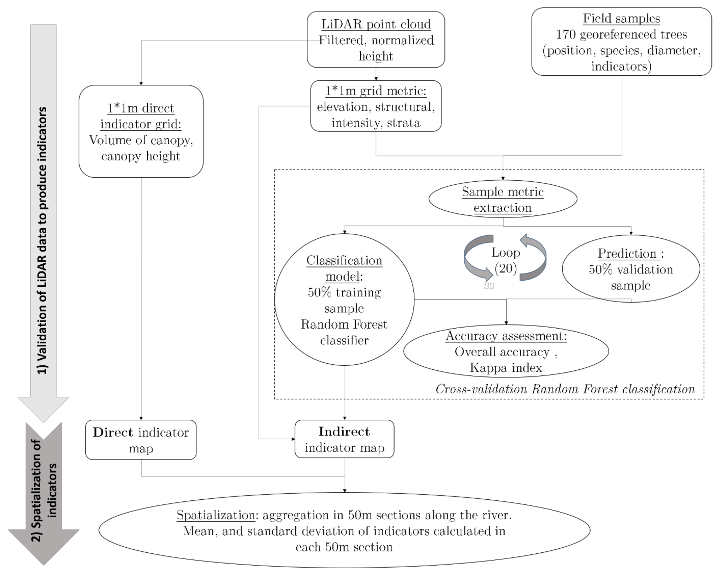
The general framework of the study (Figure 2) had two steps. The first step was to validate the use of LiDAR data to produce riparian indicators. The indicators were produced either directly from the LiDAR data or indirectly, by supervised classification of the LiDAR data. The second step consisted of spatializing these indicators and analyzing their longitudinal profile among 50 m-long sections of the riparian zone, upstream and downstream of the La Roche-qui-Boit dam. LiDAR data were validated using the entire LiDAR swath, while the indicators were spatialized only for the La Roche-qui-Boit reservoir and downstream.

2.3. LiDAR Data

The LiDAR data were acquired in June 2015 and January 2017. The data were collected with an Optech ALS Titan mounted on an aircraft flying at 400 m and in the green and NIR channels (532 and 1150 nm, respectively) (Figure 1). The sensor can record up to five discrete points per laser pulse with a high point density (Table 1).

2.4. Field Data

Seven sites along the Sélune River were investigated in the summer of 2016 and 2017. Two sites were located downstream, and five were located along the reservoir. Two sites were composed of narrow buffer strips and five were composed of floodplain forest or hillslope forest. We inventoried 170 trees of the sites’ eight main species: willow, alder, oak, ash, chestnut, lime, beech, and poplar. Tree locations were recorded with a DGPS Trimble GeoExplorer GeoXT 2005 (Trimble, Sunnyvale, California, CA, USA) with 75 cm mean horizontal accuracy. Under each tree, we recorded the crown diameter in two directions (perpendicular and parallel to the river), the number of trunks (two classes: more than two, or less than three trunk), density of the shrub stratum (three classes: low, moderate, and high), density and of the herbaceous stratum (three classes: low, moderate, and high). Among the indicators, each class contained 14–147 trees (Table 2). To validate the elevations recorded by the LiDAR sensor (Teledyne Optech, Toronto, ON, Canada), a tacheometer was used to record elevations of a bare soil site in March 2015.

2.5. Methods

2.5.1. Preprocessing and Validation of Elevation Extracted from the Bare Soil LiDAR Point Cloud

Point clouds for June 2015 and January 2017 were filtered using FUSION software (version 3.5, 2015, USDA Forest service, Pacific Northwest Station, Portland, OR, USA) [26]. The ground and other surface points were extracted with FUSION software to create a DEM (representing the terrain elevation), a digital surface model (representing the terrain elevation and that of aboveground features), and a CHM with a 50 cm spatial resolution. The last returns were considered ground points and were used to generate the DEM. The point clouds were normalized from ground points using LAStools© software (Version 120628, rapidlasso GmbH, Gilching, Germany) [27].
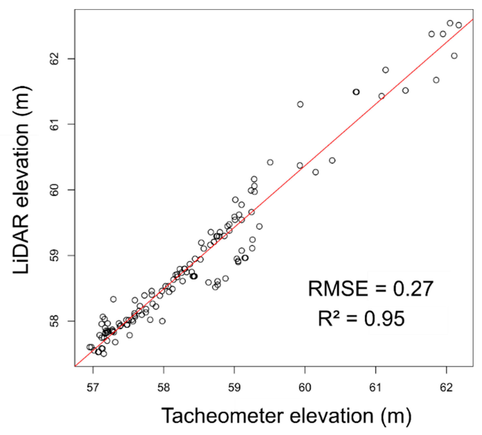
Compared to the tacheometer measurements, the elevation of the bare soil site estimated from the LiDAR point cloud had an R² of 95% and an RMSE of 0.27 m (Figure 3), suggesting a mean difference of 27 cm between true elevation (tacheometer) and LiDAR elevation. Since the study focused on riparian forest properties, the elevations the LiDAR recorded were considered sufficiently accurate.

2.5.2. Indicators of Riparian Functions

Eight indicators were extracted from LiDAR data due to their relevance in characterizing riparian function and status (Table 3). The indicators were chosen to cover a wide range of functions performed by riparian forests. The indicators were produced either directly from LiDAR data (e.g., stratification, biomass overhanging the channel) or indirectly by supervised classification of the LiDAR data (e.g., species composition, density of understory strata, and number of tree trunks).

2.5.3. Direct Indicators

Variation in canopy height can provide information about the canopy’s vertical structure [21]. The vertical structure of the canopy is strongly correlated with its species composition (some species are taller than others) and the stratification of vegetation (a homogeneous canopy is less stratified than a heterogeneous canopy). To assess vertical canopy information, the maximum, mean and standard deviation of elevation were calculated. The spatial variation in vertical structure is also related to riparian functions: a canopy’s mean height and spatial variation are related to species richness because they influence habitat diversity [1].
The overhanging character of vegetation is a crucial indicator of river status. It provides shade to the channel as well as biomass that can be used as habitats and nutrients for fish [32]. Michez et al. [21] developed an index of the area of vegetation overhanging a channel. This index is related to the continuity of the riparian corridor, the biomass overhanging the channel, and the shading it provides. It is only a 2D index, however, and biomass can be described using a 3D index. In the same way that studies estimate aboveground biomass of forests as the volume of vegetation in a given area, it is possible to estimate the biomass overhanging a river channel by calculating the volume of overhanging vegetation.
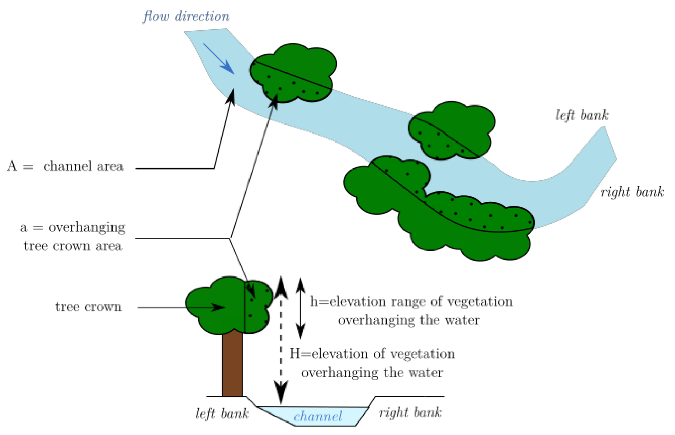
River channel area (A) was estimated using the BD TOPO® database (from the Institut Géographique National). Vegetation polygons were extracted by filtering the CHM. Overhanging vegetation polygons were extracted by intersecting the vegetation polygon with the channel polygon. Overhanging area index was calculated as the percentage of channel area overhung by vegetation. The potential volume of vegetation was estimated using the height of vegetation overhanging the channel in 1 × 1 m grid cells (H). This estimate of biomass can be biased, however, since it assumes that vegetation fills the entire space between the water surface and the maximum vegetation height. Therefore, the “true” volume of vegetation was estimated as the area of vegetation (i.e., tree crowns) overhanging the channel (a) times the elevation range of points overhanging the channel in 1 × 1 m grid cells (h) (Figure 4).

Indirect Indicators

Four indicators of riparian status were produced indirectly using supervised classification: species composition, herbaceous and shrub strata densities, and number of trunks. Species composition is correlated with habitat provision, bank stabilization, and flood regulation; for example, willow is a pioneer species that helps to stabilize banks [31]. Understory strata provide multiple functions; for example, herbaceous cover influences flood regulation [29,33] and sediment fixation [33]. Riparian tree trunks help to regulate floods by resisting flood water [33]. These indicators were produced by applying classification models to several metrics calculated from the LiDAR point cloud.
Sixteen metrics were calculated from each point cloud (leaf-on and leaf-off) (Table 4) to classify riparian species, herbaceous and shrub strata densities, and number of trunks. Leaf-on and leaf-off metrics were calculated for each 1 × 1 m grid cell using the June 2015 and January 2017 data, respectively. We divided the metrics into four categories: vertical canopy structure, strata densities, signal penetration, and spectral intensity. Elevation statistics provide information about the canopy’s vertical structure, while strata densities are related to point density in vegetation strata. Signal penetration provides information about tree biomass and density, while intensity recorded by the laser provides information about the canopy’s spectral properties.
The density of points in different strata provides information about their densities of branches and leaves. Two strata were chosen: herbaceous (0.1 cm to 1 m above the ground) and shrub (1–3 m above the ground). Ground points were excluded from the former because they can indicate short grass or bare soil. They were calculated as the percentage of points in each cell located in each stratum:
P e r c _ s h r u b = n 3 n 1 p
P e r c _ h e r b a c e o u s = n 1 n 0.001 p
where n is the number of points below the given elevation (in m), and p is the total number of points in a given cell.
Internal structure is an important characteristic of trees. Point distribution is an acceptable proxy for tree structure and has shown its utility for classification of forest species [16,39,40]. Based on the assumption that LiDAR penetrates the canopy, the laser penetration index (LPI) was used to quantify the degree of penetration [35]. LPI can be described as the number of ground points in a given cell divided by the total number of points in the cell.
The leaf area index (LAI), which characterizes the plant canopy, is widely used to distinguish species or estimate plant physiology [34,41]. Using the Beer–Lambert law, LiDAR data can provide information about the gap fraction, which is related to LAI [34]. We used the proxy for LAI of Solberg et al., [34] calculated from LiDAR data, which equals the logarithm of the number of tree points divided by the number of ground points under the tree crown. The larger the leaves are, the less the laser penetrates the canopy and reaches the ground, yielding a high index value.
The number of discrete returns of each pulse was used to characterize canopy structure. Signal penetration (P) equals the number of first returns divided by the total number of returns in a given grid cell. The mean and standard deviation of the number of returns per point (mean_N and SD_N, respectively) were also calculated. They are proxies for the degree of canopy opening: the denser the canopy, the less the LiDAR signal penetrates it.
Ratios of intensity in the green and NIR channels were calculated under leaf-on and leaf-off conditions to assess the canopy’s spectral properties. Intensity provides valuable information about the tree canopy [23,42], even though it depends on flight altitude, atmospheric conditions, and scan angle. Consequently, intensity can be difficult to interpret and analyze. However, using the ratios of two channels normalizes the intensity and decreases the influence of the flight altitude and scan angle [23].
GNDVI = i n i r i g r e e n i n i r + i g r e e n
ratio = i n i r i n i r + i g r e e n
where inir and igreen is pixel intensity in the NIR and green channel, respectively.
Random Forest [43] is a powerful algorithm used for classification [14,44] that is based on classification and regression trees but adapted to large numbers of variables and samples. It tests several of these trees with a fixed number (mtry) of randomly selected variables, called a forest, and tests their classification power. The final classification is the combination of all trees. The “randomForest” package of R software (version 3.4.1, Vienna University of Economics and Business, Vienna, Austria) [45] was used to classify riparian functions with the 32 metrics extracted from the two point clouds. Half of the samples were used for training, and the other half were used for validation. Cross-validation was performed to increase robustness of the algorithm: training and validation samples were randomly selected and used in the classification. The value of mtry was set automatically by cross-validating the training samples. Classifications were iterated 20 times using different samples. Mean overall accuracy and Kappa indices were calculated for the classification. Another advantage of the Random Forest algorithm is that it can be used to calculate the mean decrease accuracy index for each metric [43]. This index indicates the decrease in classification accuracy that would occur if the metric was removed from the dataset, allowing the metrics to be ranked according to their importance to the classification. A mean decrease accuracy index was then calculated for each indicator over the 20 classifications.

2.5.4. Longitudinal Characterization of the River

Statistics of each indicator of riparian status were calculated for 50 m sections of the interaction zone along the river: mean canopy elevation, mean standard deviation of point elevation, mean number of tree species, main tree species in the species composition, potential volume of vegetation overhanging the river, percentage of area of vegetation overhanging the river, percentage of trees with more than two trunks (class two), and mean densities of herbaceous and shrub strata (class one to three).

3. Results

3.1. Using an Indirect Approach to Map Riparian Functions

3.1.1. Metric Selection

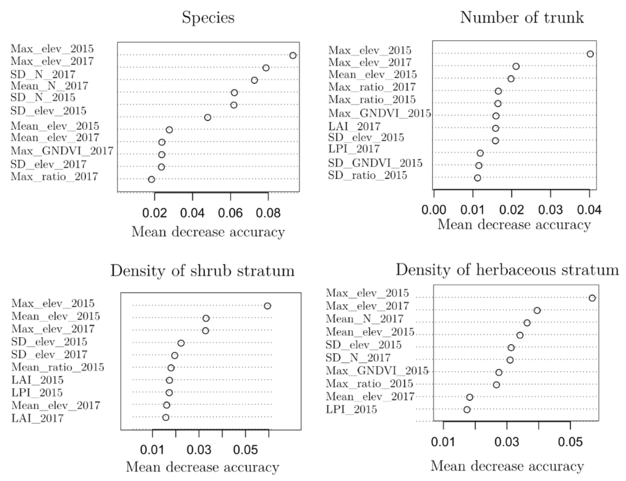
All 32 metrics were kept in the Random Forest model for the classification (Figure 5). However, the algorithm used certain metrics more frequently than others. For each indicator, the mean decrease accuracy index ranged from 0–0.1, which means that the most important variable decreased classification accuracy by only 10%. This highlights the potential complementarity of all of the metrics.
For the four indicators, the elevation metrics of both dates (leaf-on and leaf-off) were kept as the most important (i.e., highest mean decrease accuracy indexes). For species composition, six metrics were kept as important. The standard deviation and mean number of returns for the leaf-off condition were kept as the 3rd and 4th most important metric, respectively. Elevation metrics for the two dates were kept as the most important metrics for the number of trunks and shrub stratum density classifications. For herbaceous stratum density, the mean number of returns in 2017 was kept as the 3rd most important metric. The standard deviation of the number of returns in 2017 was kept as the 6th most important metric, and the maximum of GNDVI in 2015 was kept as the 7th most important metric.

3.1.2. Classification Results

The Random Forest algorithm and calculated metrics provided good results for classifying riparian indicators. Overall accuracy of species composition was 67%, while those of the other indicators were 73–88% (Table 5). Number of trunks had the highest overall accuracy (88%), as well as the lowest Kappa index (30%). Strata density was classified well, with 73% and 78% overall accuracy for the herbaceous and shrub stratum, respectively. As a test, removing the intensity metrics from the Random Forest model indicated that they had slightly influenced classification results, increasing overall accuracy and the Kappa index by six and two percentage points, respectively.

3.2. Longitudinal Characterization of the Sélune River

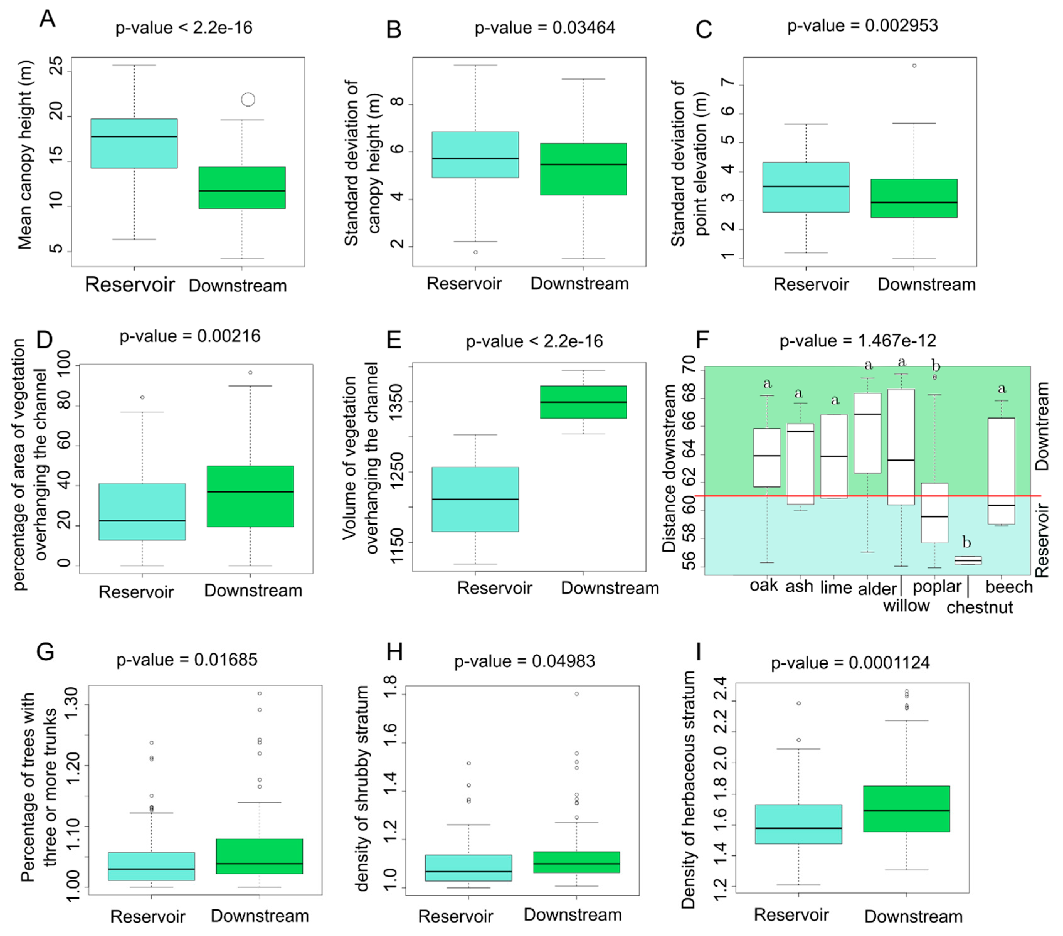
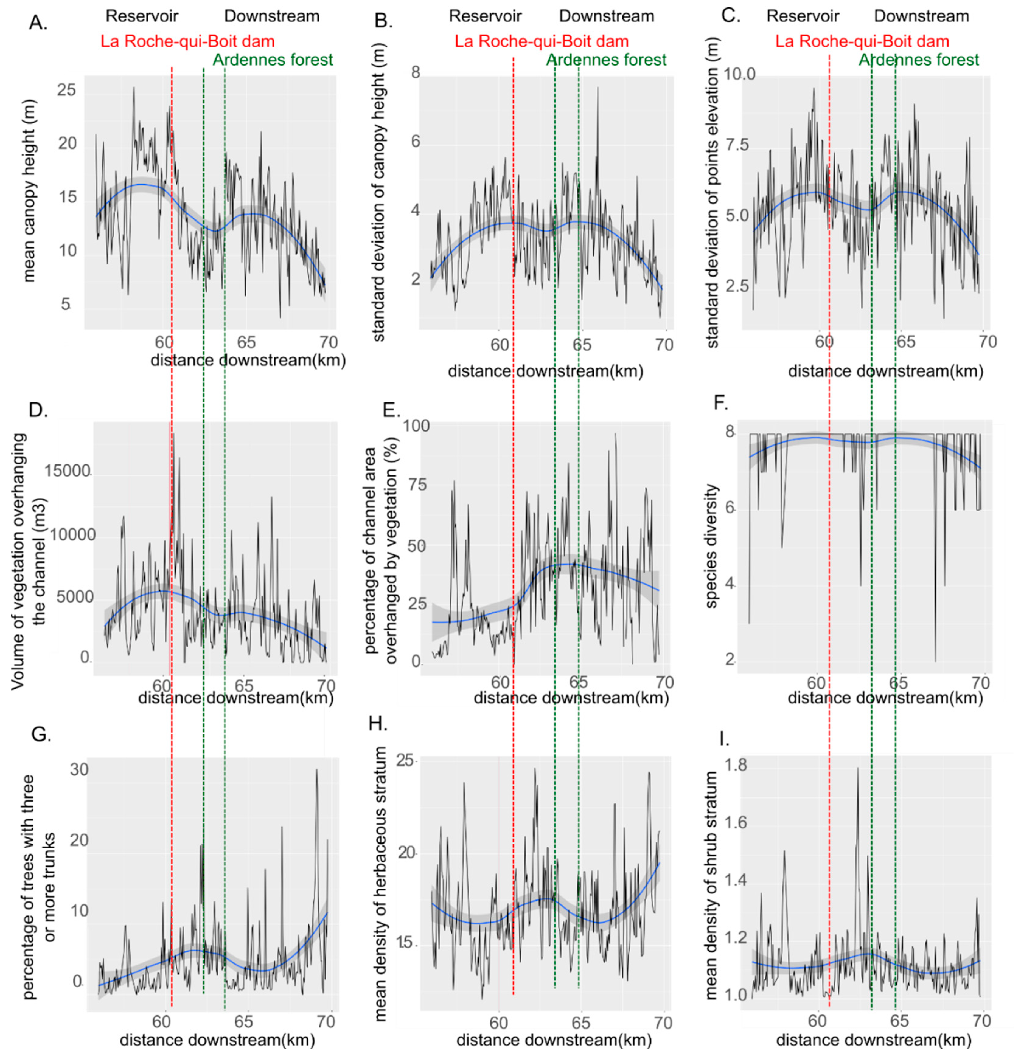
Riparian canopy was significantly taller in the reservoir (ca. 15 m) than downstream of it (Figure 6A and Figure 7A). The canopy was taller in the Ardennes forest (up to 20 m) than in the portion immediately downstream from the La-Roche-qui-Boit dam. However, the standard deviation of canopy height did not differ significantly between the reservoir and the downstream portion of the river (Figure 6B and Figure 7B). Conversely, vertical canopy structure was more diverse (i.e., higher standard deviation of point elevation) immediately upstream of the dam (Figure 6C) and downstream from it in the Ardennes forest (Figure 7C). Finally, high variability in all indicators was observed among the 50 m sections (Figure 7A–C).
The mean percentage of channel area covered by vegetation was significantly higher downstream of the dam (50% in the Ardennes forest) than upstream of the dam (10% in the reservoir) (Figure 6D and Figure 7D). Wide channel width in the reservoir and narrow channel width downstream (Figure 1) resulted in a different status for these two portions of the river, decreasing from an open channel to a narrower and shaded channel. The volume of vegetation showed a similar trend, with significantly higher volume (and thus biomass) overhanging the channel in the downstream portion (Figure 6E). The 50 m sections contained a mean of 7000 m3 of biomass. Mean volume was higher near the La Roche-qui-Boit dam (12,000 m3) than in the Ardennes forest (Figure 7E).
The river channel was composed mainly of oak, willow, and poplar, followed by chestnut and beech. Significant differences in species composition were observed along the channel (Figure 6F). Poplar and chestnut were located mainly in the reservoir upstream of the dam. Downstream, the Ardennes forest was composed mainly of oak and beech. No difference in species richness was observed among the 50 m sections (Figure 7F). Species richness varied greatly in particular locations along the length of the river sampled, suggesting diversity in local conditions.
The number of trunk differed significantly upstream and downstream of the dam (Figure 6G and Figure 7G). The percentage of trees with three or more trunks area was slightly higher in the main reservoir near the Vezins dam (ca. 20%) than downstream of it (ca. 10%).
Shrub stratum density did not differ significantly between upstream and downstream portions (Figure 6H). The 50 m sections had a mean shrub stratum density value of 1.5 (Figure 6H); however, high local variations were observed (Figure 7H). Conversely, herbaceous stratum density varied along the river. The herbaceous stratum was significantly denser in the reservoir than elsewhere (Figure 6I). Herbaceous stratum density was low in the Ardennes forest (less than 2), unlike the higher density in the open area upstream of the Ardennes forest (ca. 2.5) (Figure 7I).

4. Discussion

4.1. Contribution of LiDAR Data to Riparian Vegetation Assessment

4.1.1. 3D LiDAR Data and Indicator Production

High-precision elevation information (20 cm) was used to derive accurate CHM to calculate indicators of riparian functions. Riparian canopy vertical structure was then assessed with high precision. Similarly, LiDAR data were used to map the area and biomass overhanging the river, as done by Michez et al. [21]. The LiDAR data provided additional 3D information about biomass that would not have been available with classic optical imagery. Normalized Difference Vegetation Index (NDVI) is a good indicator of biomass, but it can become saturated and can underestimate forest biomass [46,47,48].
Maximum elevation was the most important metric for the indicator classifications. This result assumes that a simple CHM with high point density is sufficient to produce indicators of riparian status such as species composition. This result can be explained by the difference in height of certain species, such as willow (ca. 8 m) and oak or poplar (ca. 20 m) (Figure 8). Other important metrics were elevation statistics (mean and standard deviation of elevation) because the point distribution can vary according to the species or number of trunks. Willows have distinctive ball-shaped crowns with a regular point distribution, while oaks have crowns with points concentrated at the top of the tree. Similarly, point distribution differs according to stratum density. The same tree will have different point distributions (mean point elevation and standard deviation) regardless of whether the shrub stratum density is high. Simple elevation statistics alone seemed sufficient to produce indicators of riparian status. More studies are required to better analyze the influence of each metric type (CHM, elevation statistics, internal structure, signal penetration) on classification results.
Signal penetration metrics (LAI, LPI, and P) were the second most important metrics in all classifications, except for species composition classification. This highlights potential advantages of extracting more information instead of using only the CHM. Internal canopy structure seems to provide additional information useful for describing riparian forest attributes. This agrees with Lin and Hyyppä [40], who used internal canopy structure to map forest species. The indicator of biomass derived in this study assumes that canopy density is homogeneous. Information related to canopy density, such as LAI or signal penetration, could be used to weight volume information and better estimate aboveground biomass. Since aboveground biomass equals the sum of the biomass of leaves, trunks, and branches, estimating trunk and branch biomass is useful for generating a more accurate estimate. Trunk biomass can be estimated indirectly using DBH or directly using the gap in the point cloud that corresponds to the trunk [49].

Characteristics of Titan LiDAR: Bispectrum and Intensity

Beyond the advantages of using more than a CHM to extract riparian indicators, this study analyzed the potential of new LiDAR data, including multi-temporal acquisition (leaf-off and leaf-on) and bispectral information. This agrees with Brandtberg [50] and Kim et al. [51], who used both leaf-on and leaf-off datasets to classify forest species.
Conversely, inclusion of intensity metrics had no influence on classification accuracy (maximum increase of 6 percentage points), possibly because intensity was not corrected. Since intensity can vary due to a variety of parameters (scan angle, degree of signal penetration, atmospheric conditions), it is difficult to extract accurate intensity information even when using intensity ratios. Therefore, the bispectral properties of Titan are not useful for producing intensity indicators of riparian status, except for increasing point density (from both the NIR and green channels). This result does not agree with that of Antonarakis et al. [52], who used intensity and vertical canopy structure to map riparian land cover, especially poplar populations (natural, planted, and young), with greater than 80% accuracy. They did not distinguish different vegetation species, however, focusing only on poplars. Although they were able to distinguish poplars with greater than 80% accuracy, more “difficult” classes such as mature natural poplars were classified with only 66% accuracy.

4.1.2. Indirect Attributes: Specific Classification Issues

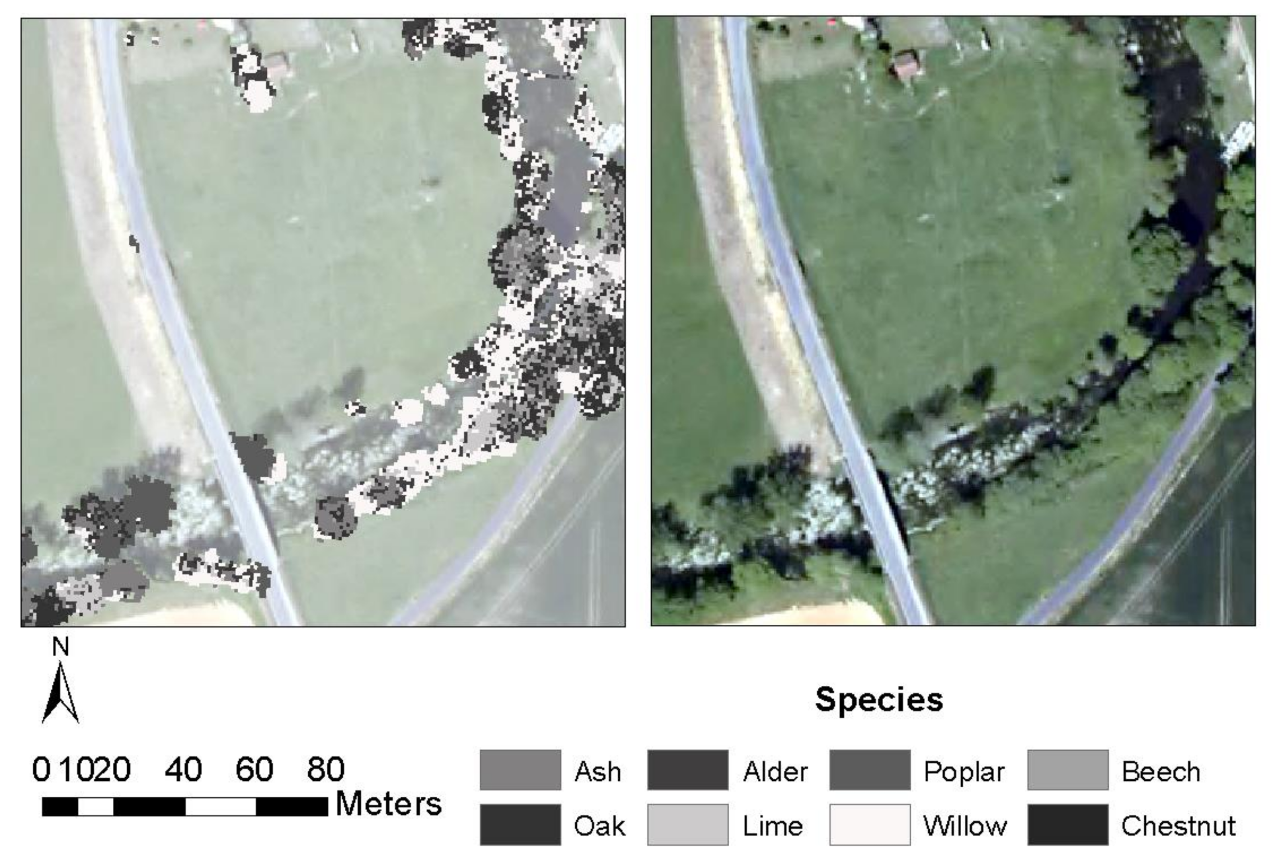
Random Forest classification models predicted the indicators of riparian properties well (≥67% accuracy). This confirms the utility of using Random Forest models to assess riparian structure. This result agrees with that of Michez et al. [14], who used Random Forest to map riparian tree species with unmanned aerial vehicles and LiDAR data with more than 80% accuracy. The maps we produced, however, had some errors. For example, several trees were classified as two or more species (Figure 9) because the top of the crown was classified as a “tall” tree such as poplar, and the external part of the crown was classified as another species. These errors can occur due to overfitting of the Random Forest algorithm, even when using cross-validation. Indeed, the Random Forest algorithm fit the training data closely, and if the predicted data have variability that is not present in the training data, the Random Forest algorithm cannot classify all of the predicted data correctly. This highlights the difficulty in building models that consider all variability observed in the field. For large areas, inventorying the entire area is not possible, or would require expensive and time-consuming effort. The results show the challenge of classifying pixel-based objects such as tree crowns. One solution is to classify tree crowns as objects instead of pixels; however, identifying trees in deciduous forests still requires field research, for no remote sensing method has yet distinguished deciduous trees well.

4.2. Longitudinal Characterization of Riparian Vegetation along a Dammed River

4.2.1. Two Compartments: The Reservoir and Downstream of the Reservoir

Longitudinal analyses revealed that riparian properties differed between the reservoir and the portion of the river downstream from it. Not surprisingly, the reservoir was more open, with lower biomass overhanging the river than that in other areas. Species composition was also significantly different in the reservoir, which contained more poplar and chestnut. The percentage of multi-trunk trees and herbaceous stratum density were significantly lower in the reservoir. The vertical structure of the canopy also differed along the river.

4.2.2. High Local Variation in Indicators

Each indicator of riparian status had high local variability, indicating that geomorphological properties of the river may have had little influence. This could be due to the particular status of the river. The river has low energy and low slope (0.02%), which results in low water and sediment transport and low geomorphological dynamics. The river is also part of a managed agricultural landscape, except for the reservoir, which is located in deep gorges. Therefore, anthropic pressure and management may influence riparian structure more than typical geomorphological variables. The type of riparian zone explained the variations better than the longitudinal distance. For example, the downstream portion of the river has buffer strips composed of tree lines, which included more willow and alder. This increase in willow in the tree lines could increase the percentage of multi-trunk trees in these parts of the river. Most willows inventoried in the field had multiple trunks, which create the particular ball shape of the species. In addition, the Ardennes forest downstream of the dam had taller trees, with greater diversity in height and greater canopy stratification than the other sections of the river. This could be due to the protected status of the forest, which belongs to the ZNIEFF (Natural area of ecological, floristic and faunistic interest) network of natural environments. Since it is a fairly old forest, it is logical that older trees are taller and are highly stratified in the tree lines of the river. This indicates that the longitudinal analyses may not have been a suitable approach to analyze riparian status patterns in a managed landscape such as the Sélune River. A finer analysis that focuses on specific riparian types may be more appropriate.

4.3. Perspective for Restoration

Previous studies of dam removal showed that it leads to exposure of dewatered sediments and creation of new riparian zones in the reservoir [53,54,55]. Consequently, the new riparian zones will likely have higher density of herbaceous and shrub strata and higher species diversity than the current area, which has mostly willow, taller vegetation overhanging the river, and higher biomass.
One issue is the behavior of the newly created floodplain, which will always be restricted by the gorges in the current reservoir. Assuming that riparian vegetation will colonize all dewatered sediments, the future riparian zone will most likely be disconnected from the agricultural landscape, which will decrease interactions between the hillslope forest and the river. According to the riparian properties observed downstream, it is likely that future riparian zones will have attributes similar to those in the Ardennes forest. Alternately, they may take a different form, with a higher density of willow that is less connected to the agricultural landscape. Future studies are required to assess the response of indicators when monitoring the evolution in riparian vegetation after dam removal.

5. Conclusions

From a methodological viewpoint, this study revealed the potential of LiDAR data to map indicators of riparian zones. LiDAR data provide direct information about riparian attributes related to elevation, such as biomass overhanging the river and the vertical structure of riparian forest. Extracting metrics related to vertical canopy structure, signal penetration, strata density, and spectral intensity help map other indicators, such as species composition and the density of herbaceous and shrub strata. These indicators are valuable for describing riparian forests before and after dam removal and for assessing the restoration.
From a thematic viewpoint, results revealed that attributes differed between the reservoir and the two sub-compartments traditionally observed with dams: upstream and downstream of the dam. Dam removal will obviously change this configuration and probably remove these differences. The Ardennes forest, observed as a specific downstream compartment, could represent the future riparian zone in the reservoir after dam removal. We focused only on the pre-restoration status of the river, however. Future studies could include the indicators produced in this study to assess the success of restoration.

Author Contributions

Conceptualization, M.L., L.H.-M. and S.D.; Data curation, M.L.; Formal analysis, M.L.; Funding acquisition, L.H.-M. and S.D.; Investigation, M.L. and S.D.; Methodology, M.L., L.H.-M. and S.D.; Project administration, S.D.; Software, M.L.; Supervision, L.H.-M. and S.D.; Validation, M.L. and S.D.; Visualization, M.LL; Writing—original draft, M.L.; Writing—review & editing, L.H.-M. and S.D.

Funding

This research was funded by the Bretagne Region and Agence de l’eau Seine Normandie for Ph.D. The Nantes Rennes LiDAR platform was funded by the Region Bretagne and the Region Pays de la Loire with European Regional Development Fund (ERDF).

Acknowledgments

The authors thank Flore Penninchx and Antoine Ba for help in the field work and data processsing. We would also like to thank Emmanuel Gouraud from GEOFIT Company, Dimitri Lague from University of Rennes 1 (Géosciences Rennes UMR 6118) and Jean Nabucet from University of Rennes 2 (LETG UMR 6554) for LiDAR data acquisition and preprocessing. We thank Mickaël and Michelle Corson for English editing.

Conflicts of Interest

The authors declare no conflict of interest. The funders had no role in the design of the study; in the collection, analyses, or interpretation of data; in the writing of the manuscript, or in the decision to publish the results.

References

  1. Naiman, R.J.; Decamps, H.; McClain, M.E. Riparia: Ecology, Conservation, and Management of Streamside Communities; Elsevier Academic Press: Burlington, ND, USA, 2010; ISBN 0-08-047068-8. [Google Scholar]
  2. Naiman, R.J.; Decamps, H.; Pollock, M.M. The Role of Riparian Corridors in Maintaining Regional Biodiversity. Ecol. Appl. 1993, 3, 209–212. [Google Scholar] [CrossRef] [PubMed] [Green Version]
  3. Tabacchi, E.; Correll, D.L.; Hauer, R.; Pinay, G.; Planty-Tabacchi, A.-M.; Wissmar, R.C. Development, maintenance and role of riparian vegetation in the river landscape. Freshw. Biol. 1998, 40, 497–516. [Google Scholar] [CrossRef]
  4. Flood risks and environmental vulnerability—Exploring the synergies between floodplain restoration, water policies and thematic policies. Available online: https://www.eea.europa.eu/publications/flood-risks-and-environmental-vulnerability (accessed on 9 August 2017).
  5. González, E.; Sher, A.A.; Tabacchi, E.; Masip, A.; Poulin, M. Restoration of riparian vegetation: A global review of implementation and evaluation approaches in the international, peer-reviewed literature. J. Environ. Manag. 2015, 158, 85–94. [Google Scholar] [CrossRef] [PubMed] [Green Version]
  6. Morandi, B.; Kail, J.; Toedter, A.; Wolter, C.; Piégay, H. Diverse Approaches to Implement and Monitor River Restoration: A Comparative Perspective in France and Germany. Environ. Manag. 2017, 60, 931–946. [Google Scholar] [CrossRef] [PubMed]
  7. Müller, F.; Hoffmann-Kroll, R.; Wiggering, H. Indicating ecosystem integrity—theoretical concepts and environmental requirements. Ecol. Model. 2000, 130, 13–23. [Google Scholar] [CrossRef]
  8. Dufour, S.; Muller, E.; Straatsma, M.; Corgne, S. Image Utilisation for the Study and Management of Riparian Vegetation: Overview and Applications. In Fluvial Remote Sensing for Science and Management; Carbonneau, P.E., Piégay, H., Eds.; John Wiley & Sons, Ltd.; Editorial office: Oxford, UK, 2012; pp. 215–239. ISBN 978-1-119-94079-1. [Google Scholar]
  9. Tullos, D.D.; Collins, M.J.; Bellmore, J.R.; Bountry, J.A.; Connolly, P.J.; Shafroth, P.B.; Wilcox, A.C. Synthesis of Common Management Concerns Associated with Dam Removal. JAWRA J. Am. Water Res. Assoc. 2016, 52, 1179–1206. [Google Scholar] [CrossRef]
  10. Akasaka, T.; Akasaka, M.; Yanagawa, H. Relative importance of the environmental factors at site and landscape scales for bats along the riparian zone. Landsc. Ecol. Eng. 2010, 6, 247–255. [Google Scholar] [CrossRef]
  11. Antonarakis, A.S.; Richards, K.S.; Brasington, J.; Bithell, M.; Muller, E. Retrieval of vegetative fluid resistance terms for rigid stems using airborne lidar. J. Geophys. Res. Biogeosci. 2008, 113, G02S07. [Google Scholar] [CrossRef]
  12. Johansen, K.; Phinn, S.; Witte, C. Mapping of riparian zone attributes using discrete return LiDAR, QuickBird and SPOT-5 imagery: Assessing accuracy and costs. Remote Sens. Environ. 2010, 114, 2679–2691. [Google Scholar] [CrossRef]
  13. Michez, A.; Piégay, H.; Jonathan, L.; Claessens, H.; Lejeune, P. Mapping of riparian invasive species with supervised classification of Unmanned Aerial System (UAS) imagery. Int. J. Appl. Earth Obs. Geoinf. 2016, 44, 88–94. [Google Scholar] [CrossRef]
  14. Michez, A.; Piégay, H.; Lisein, J.; Claessens, H.; Lejeune, P. Classification of riparian forest species and health condition using multi-temporal and hyperspatial imagery from unmanned aerial system. Environ. Monit. Assess. 2016, 188, 146. [Google Scholar] [CrossRef] [PubMed]
  15. Riedler, B.; Pernkopf, L.; Strasser, T.; Lang, S.; Smith, G. A composite indicator for assessing habitat quality of riparian forests derived from Earth observation data. Int. J. Appl. Earth Obs. Geoinf. 2015, 37, 114–123. [Google Scholar] [CrossRef]
  16. Fassnacht, F.E.; Latifi, H.; Stereńczak, K.; Modzelewska, A.; Lefsky, M.; Waser, L.T.; Straub, C.; Ghosh, A. Review of studies on tree species classification from remotely sensed data. Remote Sens. Environ. 2016, 186, 64–87. [Google Scholar] [CrossRef]
  17. Jochem, A.; Hollaus, M.; Rutzinger, M.; Höfle, B. Estimation of Aboveground Biomass in Alpine Forests: A Semi-Empirical Approach Considering Canopy Transparency Derived from Airborne LiDAR Data. Sensors 2010, 11, 278–295. [Google Scholar] [CrossRef] [PubMed] [Green Version]
  18. Kronseder, K.; Ballhorn, U.; Böhm, V.; Siegert, F. Above ground biomass estimation across forest types at different degradation levels in Central Kalimantan using LiDAR data. Int. J. Appl. Earth Obs. Geoinf. 2012, 18, 37–48. [Google Scholar] [CrossRef]
  19. Yao, W.; Krzystek, P.; Heurich, M. Tree species classification and estimation of stem volume and DBH based on single tree extraction by exploiting airborne full-waveform LiDAR data. Remote Sens. Environ. 2012, 123, 368–380. [Google Scholar] [CrossRef]
  20. Hall, R.K.; Watkins, R.L.; Heggem, D.T.; Jones, K.B.; Kaufmann, P.R.; Moore, S.B.; Gregory, S.J. Quantifying structural physical habitat attributes using LIDAR and hyperspectral imagery. Environ. Monit. Assess. 2009, 159, 63. [Google Scholar] [CrossRef] [PubMed]
  21. Michez, A.; Piégay, H.; Lejeune, P.; Claessens, H. Multi-temporal monitoring of a regional riparian buffer network (> 12,000 km) with LiDAR and photogrammetric point clouds. J. Environ. Manag. 2017, 202, 424–436. [Google Scholar] [CrossRef] [PubMed]
  22. Straatsma, M.W.; Baptist, M.J. Floodplain roughness parameterization using airborne laser scanning and spectral remote sensing. Remote Sens. Environ. 2008, 112, 1062–1080. [Google Scholar] [CrossRef]
  23. Yu, X.; Hyyppä, J.; Litkey, P.; Kaartinen, H.; Vastaranta, M.; Holopainen, M. Single-Sensor Solution to Tree Species Classification Using Multispectral Airborne Laser Scanning. Remote Sens. 2017, 9, 108. [Google Scholar] [CrossRef]
  24. Hopkinson, C.; Chasmer, L.; Gynan, C.; Mahoney, C.; Sitar, M. Multisensor and Multispectral LiDAR Characterization and Classification of a Forest Environment. Can. J. Remote Sens. 2016, 42, 501–520. [Google Scholar] [CrossRef]
  25. Alber, A.; Piégay, H. Spatial disaggregation and aggregation procedures for characterizing fluvial features at the network-scale: Application to the Rhône basin (France). Geomorphology 2011, 125, 343–360. [Google Scholar] [CrossRef]
  26. McGaughey, R.J. FUSION/LDV: Software for LIDAR Data Analysis and Visualization; US Department of Agriculture, Forest Service, Pacific Northwest Research Station: Seattle, WA, USA, 2009; p. 123.
  27. Isenburg, M. LAStools—Efficient Tools for LiDAR Processing. Version 120628; 2015; Available online: https://rapidlasso.com/ (accessed on 10 January 2019).
  28. Davies-Colley, R.J.; Meleason, M.A.; Hall, R.M.J.; Rutherford, J.C. Modelling the time course of shade, temperature, and wood recovery in streams with riparian forest restoration. N. Z. J. Mar. Freshw. Res. 2009, 43, 673–688. [Google Scholar] [CrossRef] [Green Version]
  29. Kouwen, N. Effect of Riparian Vegetation on Flow Resistance and Flood Potential. J. Hydraul. Eng. 2000, 126, 954. [Google Scholar] [CrossRef]
  30. Darby, S.E.; Thorne, C.R. Predicting Stage-Discharge Curves in Channels with Bank Vegetation. J. Hydraul. Eng. 1996, 122, 583–586. [Google Scholar] [CrossRef]
  31. Hupp, C.R. Riparian Vegetation Recovery Patterns Following Stream Channelization: A Geomorphic Perspective. Ecology 1992, 73, 1209–1226. [Google Scholar] [CrossRef]
  32. Shirvell, C.S. Role of Instream Rootwads as Juvenile Coho Salmon (Oncorhynchus kisutch) and Steelhead Trout (O. mykiss) Cover Habitat Under Varying Streamflows. Can. J. Fish. Aquat. Sci. 1990, 47, 852–861. [Google Scholar] [CrossRef]
  33. Tabacchi, E.; Lambs, L.; Guilloy, H.; Planty-Tabacchi, A.-M.; Muller, E.; Décamps, H. Impacts of riparian vegetation on hydrological processes. Hydrol. Process. 2000, 14, 2959–2976. [Google Scholar] [CrossRef]
  34. Solberg, S.; Næsset, E.; Hanssen, K.H.; Christiansen, E. Mapping defoliation during a severe insect attack on Scots pine using airborne laser scanning. Remote Sens. Environ. 2006, 102, 364–376. [Google Scholar] [CrossRef]
  35. Barilotti, A.; Sepic, F.; Abramo, E.; Crosilla, F. Improving the morphological analysis for tree extraction: a dynamic approach to lidar data. In Proceedings of the ISPRS Workshop on Laser Scanning 2007 and SilviLaser 2007, Espoo, Finland, 12–14 September 2007. [Google Scholar]
  36. Li, J.; Hu, B.; Noland, T.L. Classification of tree species based on structural features derived from high density LiDAR data. Agric. For. Meteorol. 2013, 171–172, 104–114. [Google Scholar] [CrossRef]
  37. Lindberg, E.; Eysn, L.; Hollaus, M.; Holmgren, J.; Pfeifer, N. Delineation of Tree Crowns and Tree Species Classification From Full-Waveform Airborne Laser Scanning Data Using 3-D Ellipsoidal Clustering. IEEE J. Sel. Top. Appl. Earth Obs. Remote Sens. 2014, 7, 3174–3181. [Google Scholar] [CrossRef] [Green Version]
  38. Nie, S.; Wang, C.; Zeng, H.; Xi, X.; Li, G. Above-ground biomass estimation using airborne discrete-return and full-waveform LiDAR data in a coniferous forest. Ecol. Indic. 2017, 78, 221–228. [Google Scholar] [CrossRef]
  39. Koenig, K.; Höfle, B. Full-Waveform Airborne Laser Scanning in Vegetation Studies—A Review of Point Cloud and Waveform Features for Tree Species Classification. Forests 2016, 7, 198. [Google Scholar] [CrossRef]
  40. Lin, Y.; Hyyppä, J. A comprehensive but efficient framework of proposing and validating feature parameters from airborne LiDAR data for tree species classification. Int. J. Appl. Earth Obs. Geoinf. 2016, 46, 45–55. [Google Scholar] [CrossRef]
  41. Kwak, D.-A.; Lee, W.-K.; Lee, J.-H.; Biging, G.S.; Gong, P. Detection of individual trees and estimation of tree height using LiDAR data. J. For. Res. 2007, 12, 425–434. [Google Scholar] [CrossRef]
  42. Vauhkonen, J.; Korpela, I.; Maltamo, M.; Tokola, T. Imputation of single-tree attributes using airborne laser scanning-based height, intensity, and alpha shape metrics. Remote Sens. Environ. 2010, 114, 1263–1276. [Google Scholar] [CrossRef]
  43. Breiman, L. Random Forests. Mach. Learn. 2001, 45, 5–32. [Google Scholar] [CrossRef] [Green Version]
  44. Naidoo, L.; Cho, M.A.; Mathieu, R.; Asner, G. Classification of savanna tree species, in the Greater Kruger National Park region, by integrating hyperspectral and LiDAR data in a Random Forest data mining environment. ISPRS J. Photogramm. Remote Sens. 2012, 69, 167–179. [Google Scholar] [CrossRef]
  45. Team, R.C. R: A Language and Environment for Statistical Computing; R Foundation for Statistical Computing: Vienna, Austria, 2015; ISBN 3-900051-07-0. [Google Scholar]
  46. Mutanga, O.; Skidmore, A.K. Narrow band vegetation indices overcome the saturation problem in biomass estimation. Int. J. Remote Sens. 2004, 25, 3999–4014. [Google Scholar] [CrossRef]
  47. Wang, Q.; Adiku, S.; Tenhunen, J.; Granier, A. On the relationship of NDVI with leaf area index in a deciduous forest site. Remote Sens. Environ. 2005, 94, 244–255. [Google Scholar] [CrossRef]
  48. Zhu, X.; Liu, D. Improving forest aboveground biomass estimation using seasonal Landsat NDVI time-series. ISPRS J. Photogramm. Remote Sens. 2015, 102, 222–231. [Google Scholar] [CrossRef]
  49. Harikumar, A.; Bovolo, F.; Bruzzone, L. An Internal Crown Geometric Model for Conifer Species Classification with High-Density LiDAR Data. IEEE Trans. Geosci. Remote Sens. 2017, 55, 2924–2940. [Google Scholar] [CrossRef]
  50. Brandtberg, T. Classifying individual tree species under leaf-off and leaf-on conditions using airborne lidar. ISPRS J. Photogramm. Remote Sens. 2007, 61, 325–340. [Google Scholar] [CrossRef]
  51. Kim, S.; McGaughey, R.J.; Andersen, H.-E.; Schreuder, G. Tree species differentiation using intensity data derived from leaf-on and leaf-off airborne laser scanner data. Remote Sens. Environ. 2009, 113, 1575–1586. [Google Scholar] [CrossRef]
  52. Antonarakis, A.S.; Richards, K.S.; Brasington, J. Object-based land cover classification using airborne LiDAR. Remote Sens. Environ. 2008, 112, 2988–2998. [Google Scholar] [CrossRef]
  53. Auble, G.T.; Shafroth, P.B.; Scott, M.L.; Roelle, J.E. Early Vegetation Development on an Exposed Reservoir: Implications for Dam Removal. Environ. Manag. 2007, 39, 806–818. [Google Scholar] [CrossRef] [PubMed] [Green Version]
  54. Orr, C.H.; Stanley, E.H. Vegetation development and restoration potential of drained reservoirs following dam removal in Wisconsin. River Res. Appl. 2006, 22, 281–295. [Google Scholar] [CrossRef]
  55. Shafroth, P.B.; Friedman, J.M.; Auble, G.T.; Scott, M.L.; Braatne, J.H. Potential Responses of Riparian Vegetation to Dam Removal. BioScience 2002, 52, 703–712. [Google Scholar] [CrossRef]
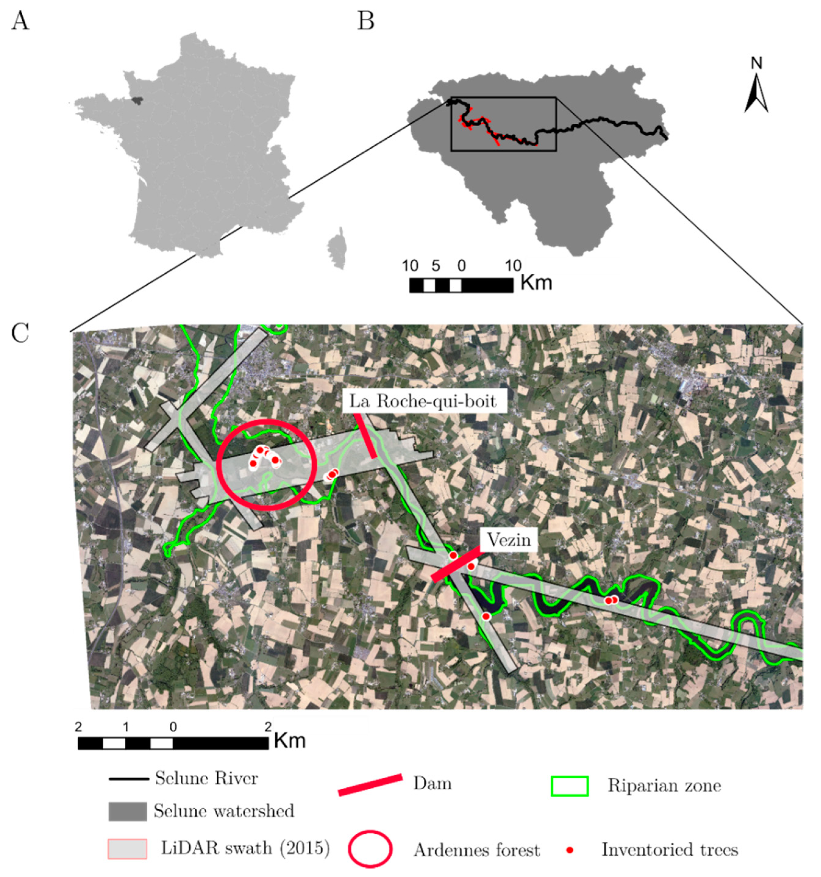
Figure 1. (A) Location of the Sélune watershed, (B) location of the study site, (C) location of the riparian zone and inventoried trees based on dam location and the Laser Detection and Ranging (LiDAR) swath.
Water 11 00483 g001
Figure 2. General framework of the study, applied to each indicator.
Water 11 00483 g002
Figure 3. Comparison of tacheometer elevation and LiDAR elevation (m) for a bare soil site.
Water 11 00483 g003
Figure 4. Estimation of the area and volume of vegetation overhanging the channel.
Water 11 00483 g004
Figure 5. Influence of metrics on classifications of riparian status indicators according to the mean decrease accuracy index (10 best metrics). See Table 4 for definitions of the metric abbreviations.
Water 11 00483 g005
Figure 6. Indicators of riparian functions upstream or downstream from the La Roche-qui-Boit dam. (A) mean canopy height, (B) standard deviation of canopy height, (C) standard deviation of point elevation, (D) percentage of channel area with overhanging vegetation, (E) volume of vegetation overhanging the channel, (F) main tree species, (G) percentage of multi-trunk trees, (H) density of the shrub stratum, (I) density of the herbaceous stratum Whiskers indicate 1.5 times the interquartile range.
Water 11 00483 g006
Figure 7. Longitudinal variation in indicators of riparian functions. The blue line corresponds to a loess smoothing function, with 95% confidence intervals represented in the gray region. (A) mean canopy height, (B) standard deviation of canopy height, (C) standard deviation of point elevation, (D) percentage of channel area with overhanging vegetation, (E) volume of vegetation overhanging the channel, (F) tree species diversity, (G) percentage of multi-trunk trees, (H) density of the shrub stratum, (I) density of the herbaceous stratum.
Water 11 00483 g007
Figure 8. 3D point cloud representation of tree species.
Water 11 00483 g008
Figure 9. Map of riparian tree species, indicating the challenge of multiple species in a single tree canopy.
Water 11 00483 g009
Table 1. LiDAR data characteristics.
ParameterConfiguration
Channel532 nm visible1064 nm near infra-red
Aircraft altitude400 m
Point density>45 points/m2
Scan angle20°
Scan frequency0–210 kHz
Pulse repetition frequency50–300 kHz
Beam divergence0.7 mrad (1/e)0.35 mrad (1/e)
Laser range precision5; <0.008 m
Accuracy (z)2.3; <5–10 cm
Table 2. Number of trees inventoried for each riparian indicator.
IndicatorAttributeClass NumberNumber of Trees
species compositionoak120
ash219
lime315
alder428
willow514
poplar631
chestnut721
beech821
number of trunksOne or two1147
more than 2223
density of shrub stratumlow1116
moderate230
high324
density of herbaceous stratumlow180
moderate269
high321
Table 3. Indicators of riparian function calculated in the study.
IndicatorMetricFunctionValidation Method
Mean canopy heightCanopy height modelSpatial heterogeneity, related to species richness [1]Elevation validation using tacheometer data
Standard deviation of canopy heightCanopy height model
Vertical canopy structureStandard deviation of point elevationVertical heterogeneity, related to habitat [3]
Area of vegetation overhanging the riverArea of vegetationShading effect, water temperature regulation [28]
Volume of vegetation overhanging the riverArea × height of vegetation
Tree species compositionSupervised classificationBiodiversity [1]Direct: field data
Density of the herbaceous stratumSupervised classification<1 m: Flood regulation, bank stabilization [29]
Density of the shrub stratumSupervised classification1–3 m: Flood regulation, habitat [30]
Number of trunksSupervised classificationFlood regulation [31]
Table 4. Metrics calculated from each of the LiDAR point clouds leaf-on (June 2015) and leaf-off (January 2017).
Type of MetricMetricAbbreviationReference
Vertical canopy structureMaximum elevationMax_elev[12,15,21]
Mean elevationMean_elev[12,15,21]
Standard deviation of elevationSD_elev[12,15,21]
Strata densitiesDensity of the herbaceous stratum: percentage of points below 1 mPerc_herbaceous--
Density of the shrub stratum: percentage of points from 1–3 mPerc_shrub--
Signal penetration Leaf area indexLAI[34]
Signal penetrationLPI[35]
Signal penetrationP[36]
Mean number of returns per pointMean_N[37]
Standard deviation of the number of returns per pointSD_N[37,38]
IntensityMean of the ratio of NIR and greenMean_ratio[23]
Maximum of the ratio of NIR and greenMax_ratio[23]
Variance of the ratio of NIR and greenVar_ratio[23]
Mean of the GNDVIMean_GNDVI[23]
Maximum of the GNDVIMax_GNDVI[23]
Variance of the GNDVIVar_GNDVI[23]
Table 5. Overall accuracy and Kappa indices for classifications of riparian function indicators using the Random Forest algorithm.
IndicatorAll MetricsWithout Intensity MetricsDifference Using Intensity Metrics
Overall Accuracy (%)Kappa (%)Overall Accuracy (%)Kappa (%)Overall Accuracy (Percentage Points)Kappa (Percentage Points)
Species composition67616255+5+6
Density of the herbaceous stratum73557253+1+2
Density of the shrub stratum78347837+0−3
Number of trunks88308831+0−1