Water Price Prediction for Increasing Market Efficiency Using Random Forest Regression: A Case Study in the Western United States

Abstract

The existence of water markets establishes water prices, promoting trading of water from low- to high-valued uses. However, market participants can face uncertainty when asking and offering prices because water rights are heterogeneous, resulting in inefficiency of the market. This paper proposes three random forest regression models (RFR) to predict water price in the western United States: a full variable set model and two reduced ones with optimal numbers of variables using a backward variable elimination (BVE) approach. Transactions of 12 semiarid states, from 1987 to 2009, and a dataset containing various predictors, were assembled. Multiple replications of k-fold cross-validation were applied to assess the model performance and their generalizability was tested on unused data. The importance of price influencing factors was then analyzed based on two plausible variable importance rankings. Results show that the RFR models have good predictive power for water price. They outperform a baseline model without leading to overfitting. Also, the higher degree of accuracy of the reduced models is insignificant, reflecting the robustness of RFR to including lower informative variables. This study suggests that, due to its ability to automatically learn from and make predictions on data, RFR-based models can aid water market participants in making more efficient decisions.

1. Introduction

Water crises, as a consequence of ever growing water demand and climate change, are now recognized as a major global challenge. Recognition of this challenge has led to increasing adoption of water markets in many of the world’s arid and semiarid regions to facilitate water transfer across competing demand [1]. The existence of water markets provides water users with clear price signals and opportunity costs that potentially enhance the economic efficiency of water use [2,3]. In a perfectly competitive market, price acts to equalize the marginal benefits from water use across users while maximizing social welfare [4]. Consequently, water prices condense information about the value of water rights that is helpful to both market participants and outsiders [5]. However, perfectly competitive water markets rarely exist in reality due to distortions such as regulatory limitations, information asymmetries, and unclear property rights, resulting in inefficient water use at the margins [6,7]. One barrier to water market participants making more efficient decisions is that few of them have sufficient and reliable information on water price, simply because the value of water rights varies with different attributes and alters with changing environmental and economic conditions. Thus, a clear understanding of water price determination and improved water price prediction can help the water markets achieve a higher degree of efficiency by allowing participants to make pragmatic purchasing and selling decisions [8,9].

Despite the benefits of studying water market price, it often faces significant challenges due to the complex relationships between price and its associated influencing factors [10]. The conventional statistical methods, such as regression analysis, have been used to measure these relationships, with emphasis either on price prediction of water transfer [11], or on explanation of water price determination [5,12,13,14,15,16]. Recently, with rapid growing requirements for big data analysis, machine-learning algorithms have become increasingly popular in studies of water resources management and hydrological sciences, due to their ability to automatically learn from and make predictions on data without explicit construction of physical or statistical models [17,18,19]. However, few applications have been reported on water rights trade issues. Although some studies attempted to use an artificial neural network (ANN) to predict price in water markets [9,20], there are still difficulties in addressing the overfitting problems [21,22].

The random forests regression (RFR) algorithm was proposed and applied to quantify complex nonlinear relationships without leading to the obvious overfitting risk [23]. RFR has been demonstrated to be more computationally cost-effective than many popular machine-learning algorithms [24]. It has been widely used for predictions of stock price [25,26,27], gold price [28], copper price [29], electricity price [30,31], property sale price [32], car resale price [33], etc. Furthermore, it has also been frequently used to handle water resources management and hydrological problems, such as reservoir inflow forecasting [19], reservoir operation [34], seasonal streamflow prediction [35,36], urban water consumption and demand prediction [37,38], flood mapping [39] and forecasting [40], drought prediction [41], weather prediction [42,43] and downscaling of precipitation [44,45]. However, to the best of our knowledge, its application on water rights trade issues has never been reported so far.

In this paper, we investigate methods of predicting the water rights price in the western United States water markets by using three RFR-based models. One is a full variable set model with all collected variables (RFR-full) and the other two are the reduced ones with optimal numbers of variables using a backward variable elimination (BVE) approach. Instead of aiming to predict the average price in water markets as conducted by other studies (e.g., [9,20]), the RFR models developed in this study have the capability to predict the price for individual water rights, considering that the water rights are heterogonous (e.g., sales vs. leases). The results showed that the RFR models had good predictive capabilities for water rights prediction, therefore can be used to help water market participants in making more efficiency decisions.

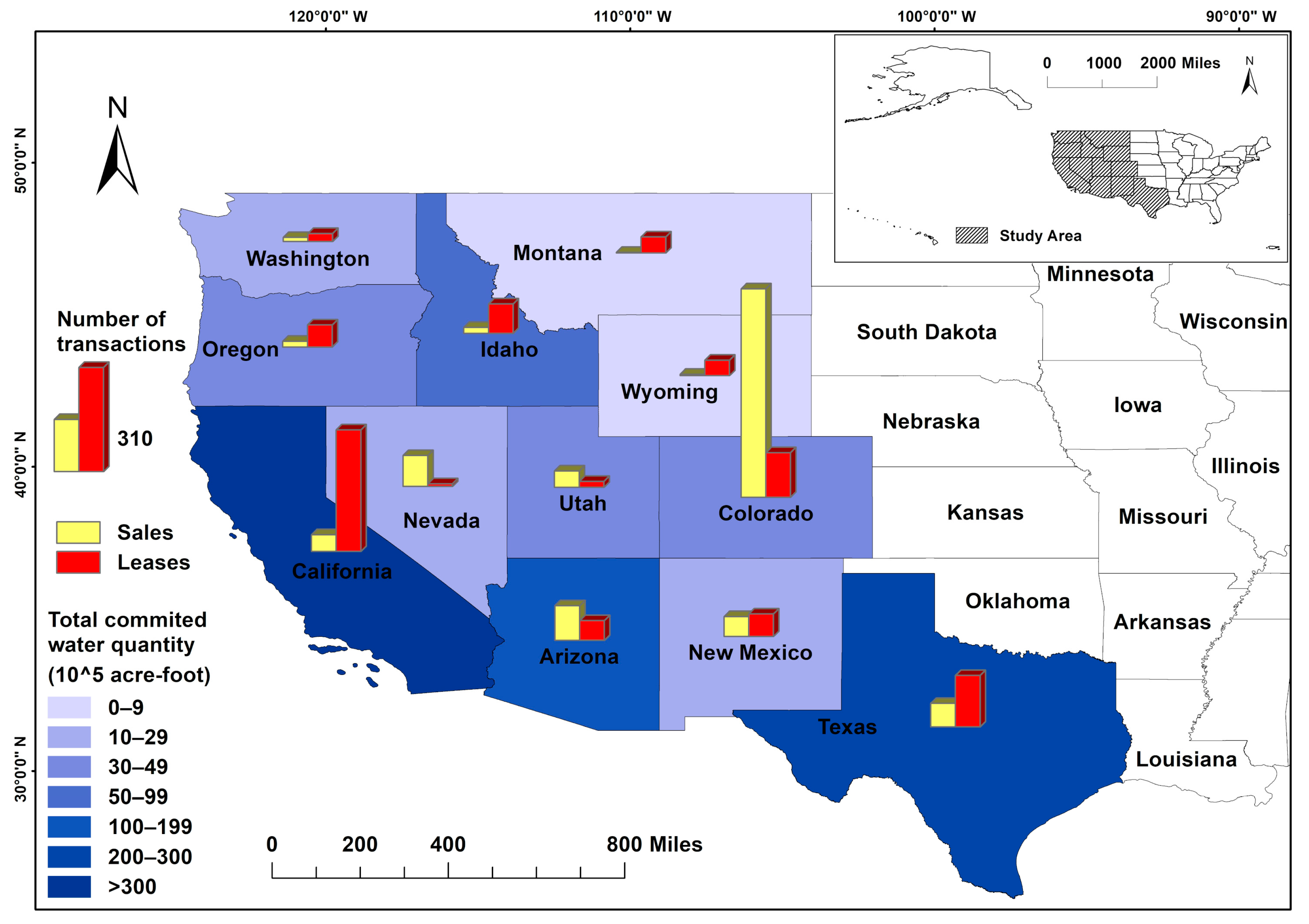
2. Study Area and Data

The study area consists of 12 states in the semiarid western United States (Figure 1). The transaction data, which spans a 23-year period, from 1987 to 2009, and includes over 4400 transactions, was originally recorded in the monthly trade journal Water Strategist and organized by Zach Donohew and Gary Libecap of the Bren School of Management at the University of California, Santa Barbara (http://www.bren.ucsb.edu/news/water_transfers.htm). Several important transaction attributes were used as predictor variables in the RFR models (

Table 1. Water rights price predictor variables and their descriptions.

Predictor Name	Predictor Description
Transaction Attributes
Direction	Prior and destination purposes of transferred water rights
Duration	Length of a contract (perpetual for sales)
Quantity	Committed volume of water sold in acre-foot
State	The state in which a transaction was made
Economics & Demographic
PerCapIn	Per capita income
PopGrow	Population growth rate
RealGDP	Real gross domestic product
IPI-Constrct	National total construction index
IPI-Other	National industry production index excluding constructions
CrpProdn	Value of crop production
FarmIn	Net farm income
Meteorological & Hydrologic
PrecipWtr	Mean precipitable water
Precip	Mean precipitation
MeanTemp	Mean temperature
MaxTemp	Mean of monthly maximum temperatures
MinTemp	Mean of monthly minimum temperatures
SnowDep	Snow depth
SWE	Snow water equivalent
CDD	Cooling degree days
HDD	Heating degree days
PDSI	Palmer drought severity index
PHDI	Palmer hydrological drought index
PMDI	Palmer modified drought index
P Z-index	Palmer Z-index
Land Uses
UrbLnd	Size of urban land use
IndusLnd	Size of industry land use
CrpLnd	Size of total cropland
EnvLnd	Size of environmental land use
GrassLnd	Size of grassland for pasture

). First is the Direction, which is classified by the prior and destination purposes of the transferred water rights. The second variable is the Duration, which is also termed as contractual form or transfer type in other literature (e.g., [46,47]). We classified duration as sale (permanent transfer), one-year lease, mid-term lease (2–10 years) and long-term lease (more than 10 years). The third attribute Quantity captures the quantity of water traded in unit of acre-foot (AF). Following Brewer et al. [46], we applied the committed water quantity, which projects the annual amount of water forward for the duration of the multi-year leases and considers the fact that the sales are perpetual. The committed quantity allowed us to make a comparison between water sales and leases in terms of unit price (in dollars per committed AF). The last attribute variable State represents the location where a transaction was made.

Other potential predictor variables of water price were also assembled for this study. The candidate variables were selected based on our knowledge and previous works (e.g., [5,11,16,48]). Population growth data for each state were obtained from the U.S. Census Bureau. Per capita income and real gross domestic product (GDP) data were collected from the U.S. Bureau of Economic Analysis. The value of crop production data and land use data were obtained from the US Department of Agriculture (USDA), while the two industry production indices were collected from the Organization for Economic Co-operation and Development. Because the land use data were updated every five years, linear interpolation was used to construct the synthetic annual land use data. Several seasonal state-level meteorological and hydrologic variables were constructed to capture the response of water price to the changing weather conditions. Specifically, the snow data were averaged over the mountain observations with seasonal delay from USDA-NRCS SNOTEL sites. The precipitation and temperature-related variables were computed from monthly observations, and the precipitable water and drought indices were calculated from daily data at 2.5 degree global grid. These data were gathered from the National Oceanic and Atmospheric Administration.

Some adjustments were made to the data assembly. Firstly, all monetary data were converted to the year 2009 dollar using the consumer price index provided by the U.S. Bureau of Labor Statistics. Secondly, crop production value, net farm income and land use data were normalized respectively using the Z-score for each state, so that their values were adjusted to a notionally common scale across states. Finally, trading data with missing price or unknown direction were excluded. The simple statistics of the adjusted prices from the remaining 2821 observations are summarized in Tables S1 and S2.

3. Methods

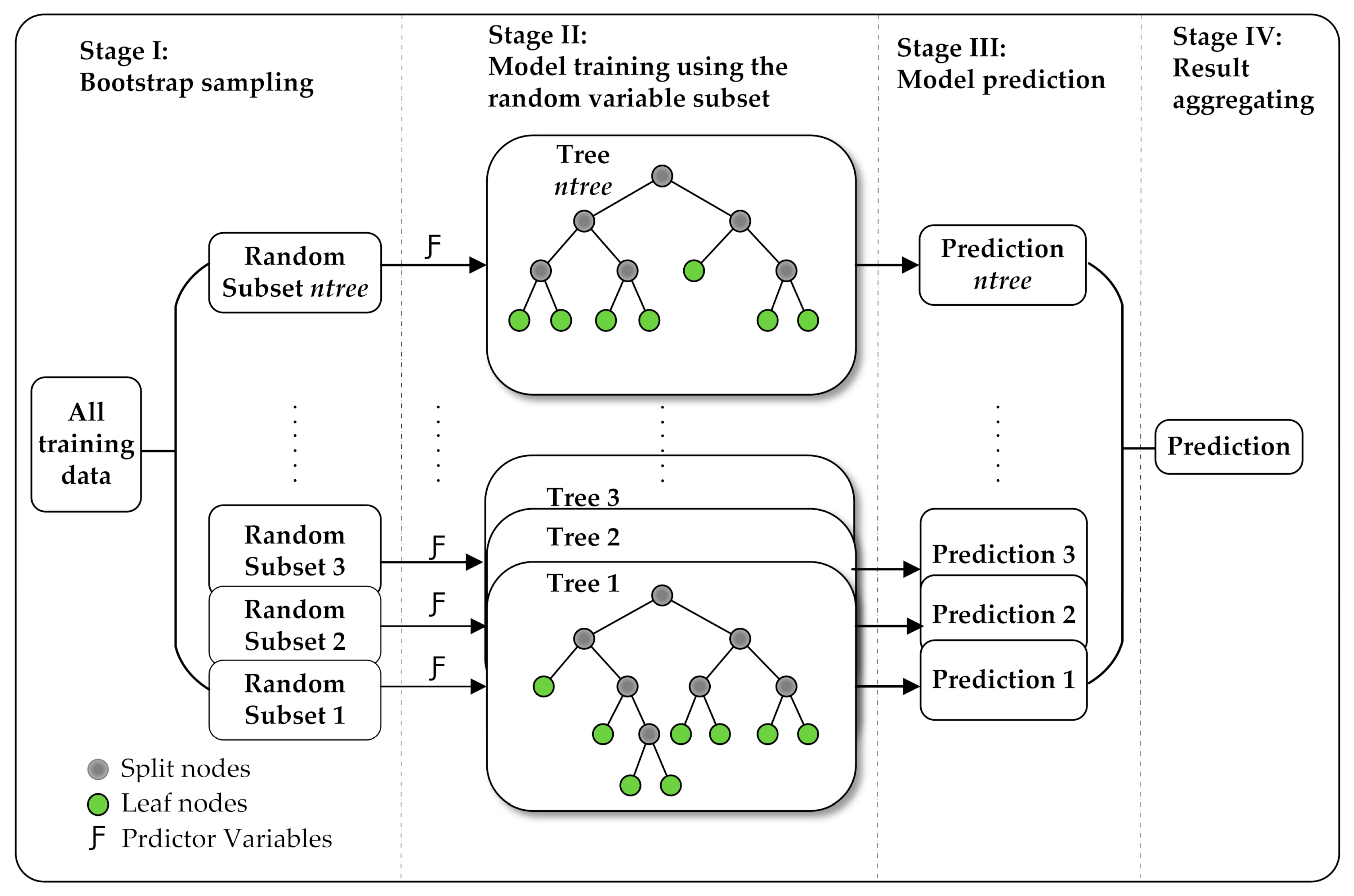
3.1. Random Forest Regression

The random forest regression (RFR) is a nonparametric ensemble learning algorithm that constructs a multitude of standard decision trees at the training process and outputs mean prediction of the individual trees [23,49] (Figure 2). A decision tree is a hierarchical analysis diagram in which each internal (split) node represents a test function on one independent variable, each branch represents the test outcome and each terminal (leaf) node represents a decision. Specifically, at each internal node, the algorithm searches the values of the incoming dataset and recognizes a threshold for one predictor variable to split the dataset such that the homogeneity of dependent variable values in each branch is maximized.

In the RFR, each decision tree is trained using a subset of data randomly sampled with replacement from the original training dataset, which can increase the robustness against overfitting [50]. In order to inject an additional layer of randomness, instead of using all variables, only a subset of randomly selected variables are considered to form the split nodes of each tree [51]. The reason to add this randomness is to reduce the redundancy of predictor variables while increasing the diversity of the trees in a forest [52]. The final result of RFR is decided by aggregating predictions of each individual tree. The RFR algorithm has four steps described as follows:

(1)

Use the bootstrap method to produce n_tree subset samples from the original training dataset, where n_tree is the number of trees to grow.

(2)

Grow regression trees on each bootstrap sample, during which, randomly draw a subset containing m_try predictor variables at each splitting node and determine the optimal split based on this subset of variables only. This process is conducted recursively until a stopping criterion (nodesize) is reached.

(3)

Obtain regression predictions over n_tree decision trees. For each individual tree, the prediction is the mean of the dependent variable values at the corresponding leaf nodes.

(4)

Compute the final prediction by averaging n_tree predictions in the forest.

3.2. Model Hyperparameter Optimization

In the field of machine learning, a hyperparameter is a parameter whose value is tuned either to improve model performance or to decrease the time and memory cost of running. The model performance is the only aspect considered in this paper. The three main hyperparameters in RFR that can influence the model’s performance are n_tree, m_try and nodesize. As mentioned earlier, n_tree is the number of trees in a forest. Larger n_tree can increase the stability of models and predictor importance estimates while decreasing the degree of overfitting, but requires more computational resources [51]. The second hyperparameter m_try is the number of variables available for splitting at each tree node, which determines the diversity among decision trees. Lastly, nodesize is the minimal size of the leaf nodes, which is used as a stopping criterion and controls the depth of the trees.

Two strategies are widely used to validate models when tuning hyperparameters in machine learning. First is k-fold cross validation (CV), in which multiple rounds of validation are performed using different partitions of a dataset, and the final result is averaged over the k rounds to evaluate the model performance. The second strategy is to evaluate trained RFR using out-of-bag (OOB) data, which is the data (approximately one third of total data) not drawn by bootstrapping for growing an individual tree at the training stage. Usually, CV is more reliable since it overcomes the fact that the model performance can be very sensitive to how training and validation subsets are divided, but OOB requires shorter runtime. To reduce the risk of overfitting, this study combines these two strategies for searching the optimal hyperparameter sets, which has two steps described as follows:

(1)

For each round of CV, tune hyperparameters using the grid search method to minimize the OOB error within the training dataset.

(2)

Assign the hyperparameter combinations with the lowest OOB errors to each of the k models and test their performances using their corresponding validation datasets. The hyperparameter combination that has the best model performance is the final model configuration.

3.3. Variable Importance Metrics

We quantify each variable’s relative contribution to the predictive models based on two types of variable importance (VI) metrics. The first one is the permutation-based VI (PVI) metric; it is one of the most robust and commonly used VI scores for RFR. The idea behind the PVI metric is to shuffle (randomly permute) all values of a variable F_j, and the importance score of F_j is defined as the reduction in model predictive performance after the shuffling (permutation) [23]. That is, if a variable is not useful in predicting an outcome, then shuffling its values will not alter the final model performance [52]. In many software packages, predictive accuracy is defined as mean squared error (MSE). The importance for the jth variable F_j in tree ϕ_t is defined as

$$V{I}_t(F_j)=\frac{MSE({\widehat{Y}}_t,Y_t)-MSE({\widehat{Y}}_t^{(j)},Y_t)}{MSE({\widehat{Y}}_t,Y_t)}\times 100\%$$

(1)

where Y_t denotes the OOB data of ϕ_t (for t = 1,…, n_tree), and Ŷ_t and Ŷ_t^(j) denote the corresponding OOB predictions before and after permuting F_j, respectively. The overall importance for variable F_j is computed as the mean of the VI over all trees in the forest,

$$VI(F_j)={\displaystyle \sum _{t=1}^{n_{tree}}VI{}_t(F_j)}/n_{tree}$$

(2)

Another VI metric is the node impurity based VI (NVI) metric. Node impurity measures the homogeneity of the response values (water price in this study) at a node. Because each internal node in a decision tree is a condition on a single variable; it is designed to split the incoming training dataset so that similar response values end up on the same branch, thus the impurity will always decrease after a split. The impurity reduction at any parent node is the difference between the impurity before the split and the weighted sum of impurity of the daughter nodes. Normally, node impurity for RFR is measured by residual sum of squares (RSS). The decreased impurity for node p in any tree is as follows:

$$\Delta RSS(p)=RSS(p)-{\displaystyle \sum _{d=1}^D{\omega }_{d}RSS(d)}$$

(3)

where d denotes the daughter node of p, and w_d represents some weight associated with node d. The VI of F_j is defined as the total weighted increase in node purities for all nodes p where F_j was used for partitioning, averaged over all trees in the forest [23],

$$VI(F_j)=\frac{1}{n_{tree}}{\displaystyle \sum _{t=1}^{n_{tree}}{\displaystyle \sum _{p\in {\varphi }_t}1[\upsilon (S_p)=F_j]}}[\omega (p)\Delta RSS(p)]$$

(4)

where ν(S_p) denotes the variable used to split node p, and ω(p) is the proportion of samples reaching node p to the total training sample of the tree.

3.4. Model Performance Indices

Three performance indices were used to evaluate the predictive accuracy of the RFR models, i.e., Pearson correlation coefficient (PCC), coefficient of determination (R²), and normalized root mean squared error (NRMSE). PCC is defined as:

$$PCC={\displaystyle \sum _{}^V(Y-\overline{Y})}(\widehat{Y}-\overline{\widehat{Y}})/\sqrt{{(Y-\overline{Y})}^2{(\widehat{Y}-\overline{\widehat{Y}})}^2}$$

(5)

Mathematically, PCC is the squared root of R². The latter is defined as follows:

$$R^2={\displaystyle \sum _{}^V{(\widehat{Y}-\overline{Y})}^2}/{\displaystyle \sum _{}^V{(Y-\overline{Y})}^2}$$

(6)

where Y and $\overline{Y}$ denote the ith observation and mean of a sample, respectively; Ŷ and $\overline{\widehat{Y}}$ denote the corresponding predictions and the mean of predictions, respectively; V represents the sample size.

$$NRMSE=\sqrt{\frac{1}{V}{\displaystyle \sum _{}^V{(Y-\widehat{Y})}^2}}/(Y_{max}-Y_{min})$$

(7)

where Y_max and Y_min are the maximum and minimum values in a sample.

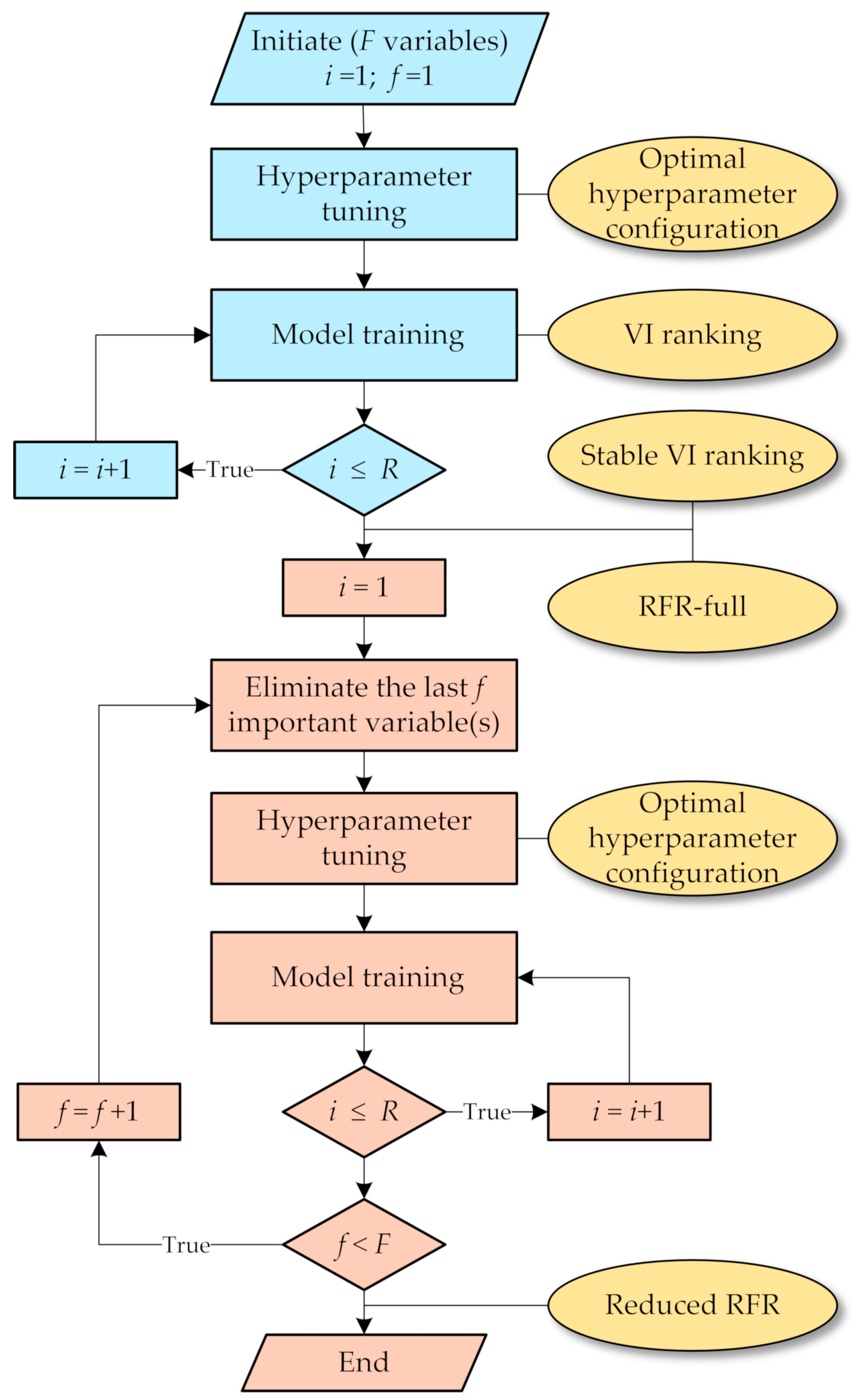
3.5. Stepwise Model Selection

This study proposes a stepwise model selection procedure called backward variable elimination (BVE) to develop the reduced RFR models (Figure 3), which is described as follows:

(1)

Obtain the optimal hyperparameter configuration of RFR-full as described in Section 3.2. Compute the VI scores of the F variables based on the optimal hyperparameters. Average VI scores over R replications to acquire a stable VI ranking.

(2)

Build a stepwise series of F−1 RFR models by iteratively eliminating the last f important variable(s). That is, according to the finalized ranking, discard the least important variable in the first round (when f = 1), and continue to remove the next important variable until a series of RFR models with F−1, F−2,…, 1 variables are constructed. For each model, an optimal hyperparameter set is selected and the model is trained R times.

(3)

Evaluate the series of RFR models by averaging their performances over the R runs. The optimal RFR reduced model is the one with the highest predictive performance.

4. Results and Discussion

The algorithms were implemented in the R computer language on an 8-core processor in our study. We set the number of replications to R = 8, as multiple runs can be processed simultaneously. According to the number of data, we chose k = 10 for the CV. The data from 1987 to 2008 were used for the training and validation processes, in which the performances of four models were assessed. Then, the 2009 data were used as a testing subset to evaluate the models’ generalization. The four modes are:

(1)

The full variable set RFR model (RFR-full);

(2)

The optimal reduced RFR developed based on the PVI metric (RFR-red-P);

(3)

The optimal reduced RFR developed based on the NVI metric (RFR-red-N);

(4)

A single decision tree model (DT), which was used as a baseline model. It was programmed based on the R part package in the R computer language.

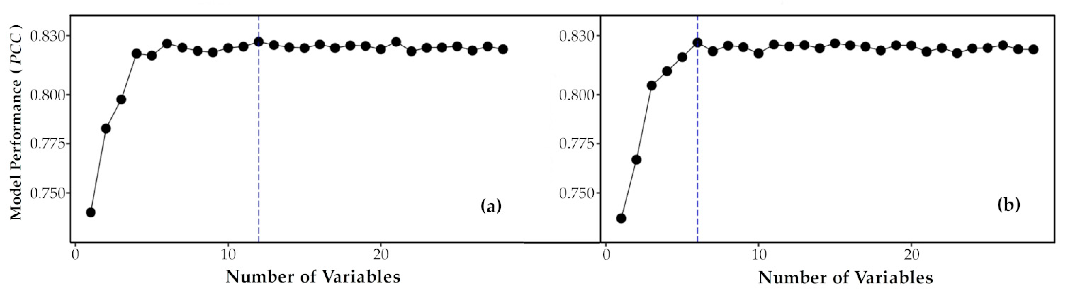
4.1. Optimal Numbers of Variables

The predictive accuracy curves shown in Figure 4 were constructed from the 8-run averaged PCC values between the actual prices and predicted prices generated by each reduced model. The RFR-red-N and RFR-red-P were identified when 12 and 6 predictor variables remained in the BVE procedure, respectively. It shows that when the variables are removed at each step, the model accuracies fluctuate steadily until the optimal points are reached. The accuracy curve declines rapidly from the optimal point as more variables are discarded with the PVI ranking, whereas it remains relatively stable for the next several variables with the NVI ranking.

In general, the reduced RFR models with more than 6 predictor variables have similar predictive power (PCC > 0.80). This is consistent with the claim that RFR algorithm is robust to including many low-informative or even noisy variables [23,53]. Interestingly, it reveals that although the optimal number of variable differs as different VI metrics are applied; the metric selection does not necessarily lead to substantial difference in prediction accuracy between models with similar variable numbers. This implies that the predictive performances of the reduced models are not sensitive to which VI metric is applied in the BVE procedure.

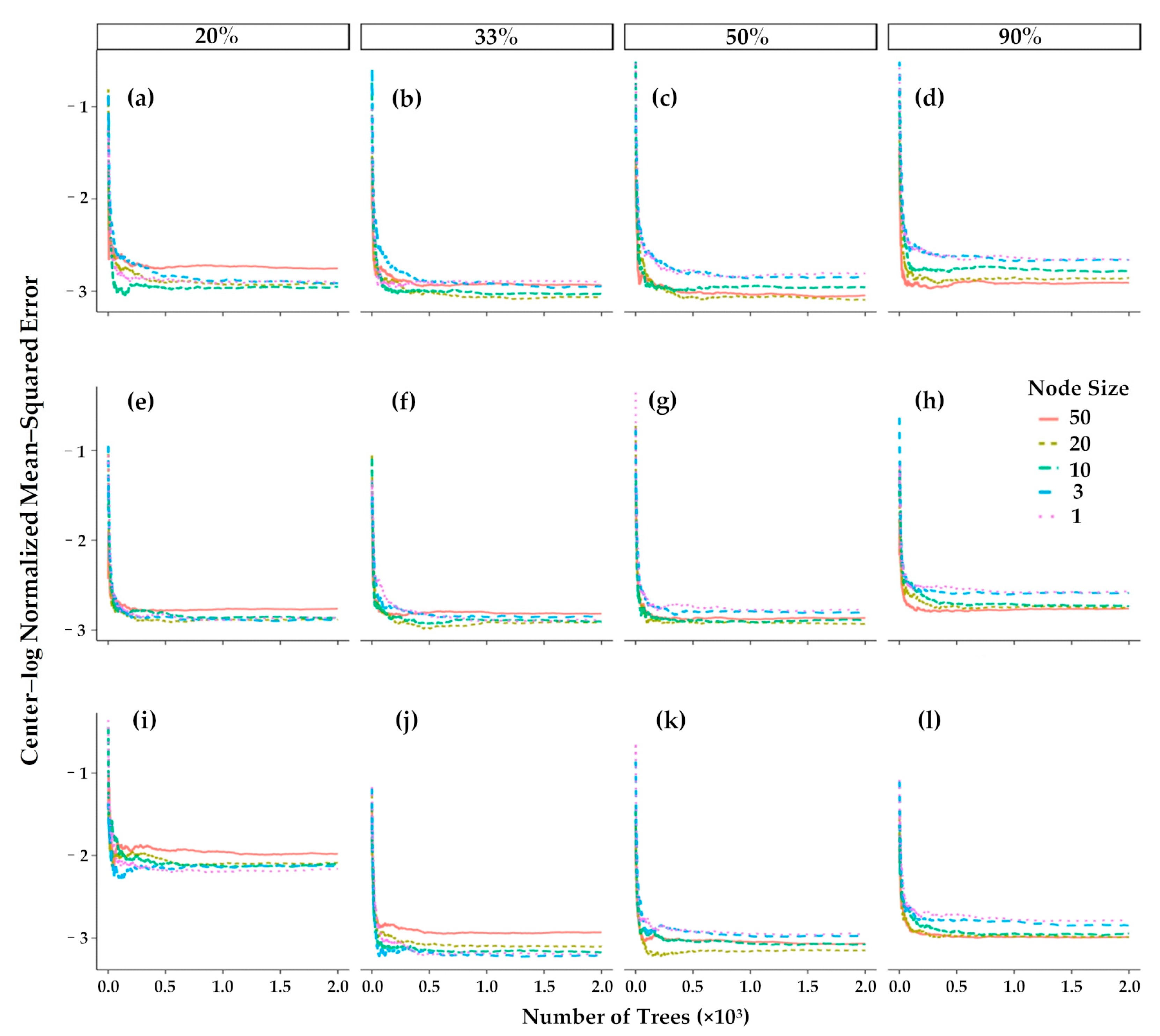
4.2. Optimal Hyperparameters

As noted earlier, n_tree, m_try and nodesize were optimized with a traditional grid search approach to increase the RFR models’ predictive power. We swept for the optimal n_tree from 1 to 2000, with an increment of one tree at each time. The best nodesize was searched among the discrete options of 1, 3, 10, 20, 50, and m_try took 20%, 33%, 50% and 90% of the total number of variables (rounded down). During each tuning process, model performance was computed based on each of the hyperparameter grids in the 3-D space. The highest OOB error was normalized to unity (baseline scenario) while the errors under other scenarios were normalized to a proportion of the baseline error.

Figure 5 illustrates the scaled error curves for the RFR-full, RFR-red-P and RFR-red-N with different hyperparameters combinations. Most of the error curves converge quickly as the numbers of trees exceed a relatively small value, indicating that when an adequate number of trees are grown, the improvement of price predictive accuracy in the water markets obtained by adding more trees diminishes. However, we still suggest growing more trees for water price prediction in future studies, especially when tuning is not included, because the optimal n_tree may strongly depend on the dataset properties. Also, growing more trees typically can improve model performance [54].

While many software packages set F/3 as a default value for m_try with F being the total number of predictor variables, our result indicates that m_try with values different from this default setting sometimes can obtain higher model accuracy. This is consistent with the experiments conducted by [55], which also illustrates that this default value of m_try is reasonable but can be improved. The final optimal hyperparameter configurations for the full and optimal reduced models are reported in

Table 2. The optimal hyperparameter configurations of the RFR models.

Models	ntree	mtry	nodesize
RFR-full	1876	15 (50%)	20
RFR-red-N	452	4 (33%)	20
RFR-red-P	109	2 (33%)	3

. It is worth mentioning that, to increase the overall model performances and the computational efficiency, many other techniques may be applied in searching the globally optimal hyperparameter configuration. Various heuristic optimization algorithms such as genetic algorithm and simulated annealing and some more advanced methods have been used in the training of machine learning-based models in previous studies [56].

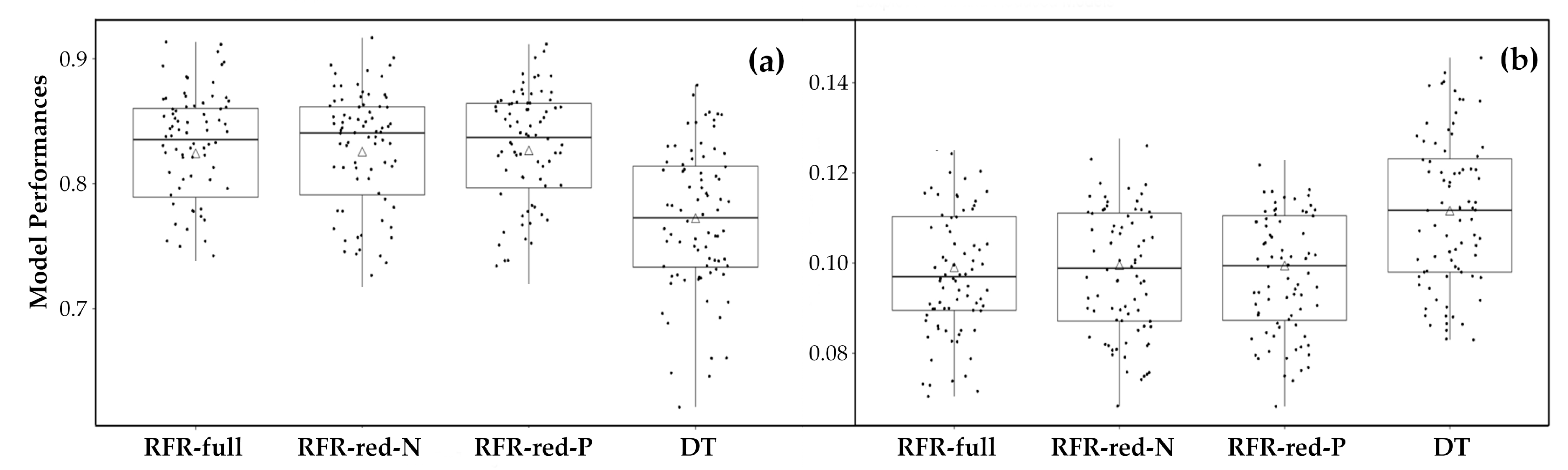
4.3. Model Performances

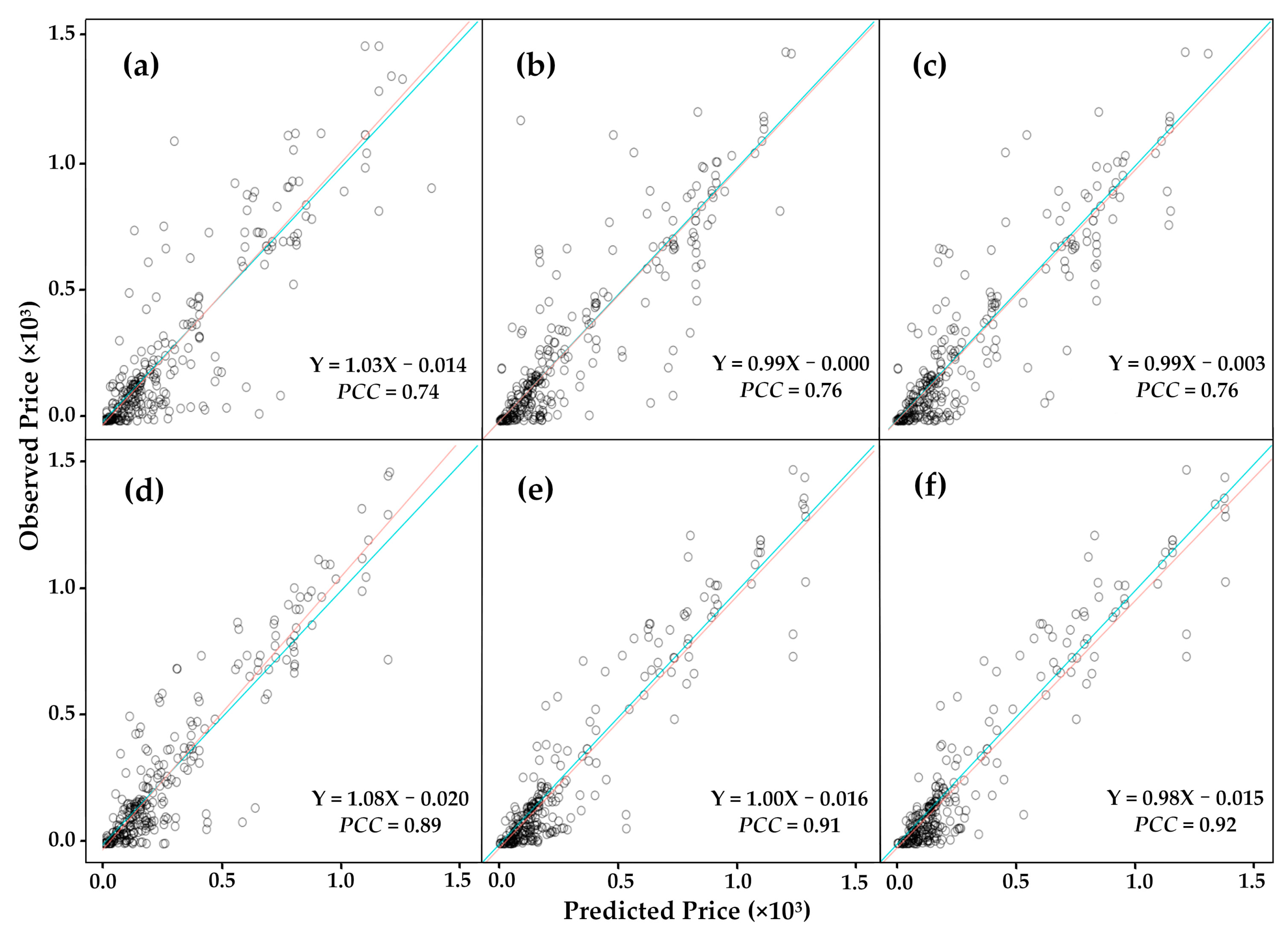
4.3.1. Predictive Accuracy

The predictive performances of the RFR-full and two optimal reduced models were assessed based on the three accuracy indices given in Section 3.4.

Table 3. Predictive performances of the RFR and baseline models.

Models	PCC		R2		NRMSE
	Mean 1	Maximum 2	Mean 1	Maximum 2	Mean 1	Minimum 2
RFR-full	0.832	0.900	0.692	0.810	0.093	0.069
RFR-red-N	0.836	0.912	0.699	0.832	0.094	0.066
RFR-red-P	0.841	0.920	0.707	0.846	0.091	0.065
DT (baseline)	0.736	0.805	0.541	0.648	0.118	0.089

¹ Averaged results over all validation rounds; ² Averaged results over the best validation rounds in each of the CV replications.

shows the overall model performance scores that were aggregated from the 8 CV repetitions. The result demonstrates that the RFR-red-P (PCC = 0.841; R² = 0.707; NRMSE = 0.091) slightly outperforms the other two RFR models, followed by RFR-red-N (PCC = 0.836; R² = 0.699; NRMSE = 0.094). RFR-full exhibits relative less predictive power (PCC = 0.832; R² = 0.692; NRMSE = 0.093). In addition, the highest predictive accuracies in each of the CV replications were also averaged to estimate the best predictive performance the models can achieve within the training and validation datasets. The better performance of the two reduced models proves the advantage of filtering out variables with low to moderate VI. However, the improvement in mean and best predictive accuracies as a result of predictor reduction using BVE is not significant. In fact, applications of random forests in other fields (e.g., [53,57]) have also found that the models with reduced numbers of variables only have equivalent or slightly better predictive performance than models without variable filtering. Not surprisingly, all the RFR models outperform the baseline model significantly, reflecting the ability of the ensemble bagging algorithm to obtain better predictive performance than could be obtained from any of the constituent learning algorithms alone.

4.3.2. Model Reliability

The reliability of the RFR models was also investigated. Here, the reliability is defined as the model’s ability to generate water price predictions with a similar level of accuracy regardless of how training and validation subsets are partitioned. To assess the reliability of the models, the coefficient of variation (CoV) of model accuracies from the multiple CV rounds were computed (

Table 4. Coefficient of variations of model accuracies of the RFR and baseline models.

Models	PCC	R2	NRMSE
RFR-full	6.21%	11.90%	15.03%
RFR-red-N	6.31%	12.75%	15.91%
RFR-red-P	6.44%	12.62%	15.88%
DT (baseline)	7.63%	13.09%	16.33%

). It shows that the variation among predictive accuracies using RFR-full is relatively lower than that using the reduced ones. This demonstrates that the RFR is more reliable as more predictor variables are available. That is, decreased diversity among decision trees as a consequence of smaller number of total available variables may influence the model reliability. However, the difference in model reliability among the RFR models is not significant, which further reflects that the RFR is robust to including some low-informative variables. Overall, all RFR models outperform the baseline DT model in terms of stability.

We also constructed jitter boxplots for each model to visually compare the distribution of their predictive accuracies (Figure 6). The boxplots illustrate that the predictive accuracies of the three RFR models follow similar distributions. This further reveals that the BVE procedure does not significantly improve the model performances. All the models performed stably as no outliers are identified in any boxplot, and thus they are considered reliable for water rights price prediction within the dataset.

4.3.3. Consistency and Bias between Observations and Predictions

To further evaluate the performance of the RFR models, ordinary least squared regression analysis was conducted to quantify the degree of similarity between the observed and predicted water prices. The regression equations (Ŷ_i = bY_i + a) of the paired observations and predictions from each of the 80 validation rounds were plotted and computed for each RFR model (an example is given in Figure 7). Since the slope and intercept of a regression equation describe the consistency and bias between the observations and predictions, respectively [58], this study tested (1) whether the slopes from each model were not significantly different from one (H₀: b = 1) and (2) whether the intercepts from each model were not significantly different from zero (H₀: a = 0). The result of the hypothesis tests is given in

Table 5. Regression parameters and hypothesis testing for the RFR models (Degree of freedom = 79).

Models	Test b (Slope) = 1		Test a (Intercept) = 0
	t Statistic	p-Value	t Statistic	p-Value
RFR-full	−1.270	0.201	0.360	0.720
RFR-red-N	0.698	0.487	−0.305	0.761
RFR-red-P	0.794	0.430	0.614	0.541

. It shows that both the null hypotheses for slope and intercept are failed to be rejected at 5% significance levels, which statistically proves that the predicted price of water transfer generated by the RFR models are unbiased and consistent with their observed values.

4.3.4. Model Generalization

The goal in machine learning is that the model can perform well on new or previously unseen inputs. That is, a trained model is able to achieve good results when it is applied. The ability to perform well on unobserved inputs is called generalization [59]. The generalization of the RFR models was tested to predict the prices of the water transfers in 2009, which is the out-of-sample data that was not used during the training and validation processes. The optimal RFR models were built during training and validation based on the 1987–2008 dataset, and then the new input data of the predictor variables were loaded into the program to generate price predictions.

Table 6. Performance of the RFR and baseline models as applied to predict water price for 2009.

Models	PCC	R2	NRMSE
RFR-full	0.875	0.766	0.083
RFR-red-N	0.908	0.824	0.067
RFR-red-P	0.917	0.841	0.063
DT (baseline)	0.116	0.013	0.364

presents the result for the model generalization test. It shows that the three RFR models have good predictive capability with performance scores that are close to their CV results. However, despite the fact the baseline model shows acceptable performance during validation, its predictive performance scores in the testing process are exceptionally low, indicating that the trained DT model seriously overfits and, given the unused inputs, has almost no predictive power for water price. It comes as no surprise that overfitting only occurred in the DT among the four models studied, as single decision trees are prone to overfitting, particularly when the trees are fully grown. On the other hand, RFR is robust against overfitting as one goal of ensemble methods is to improve generalizability.

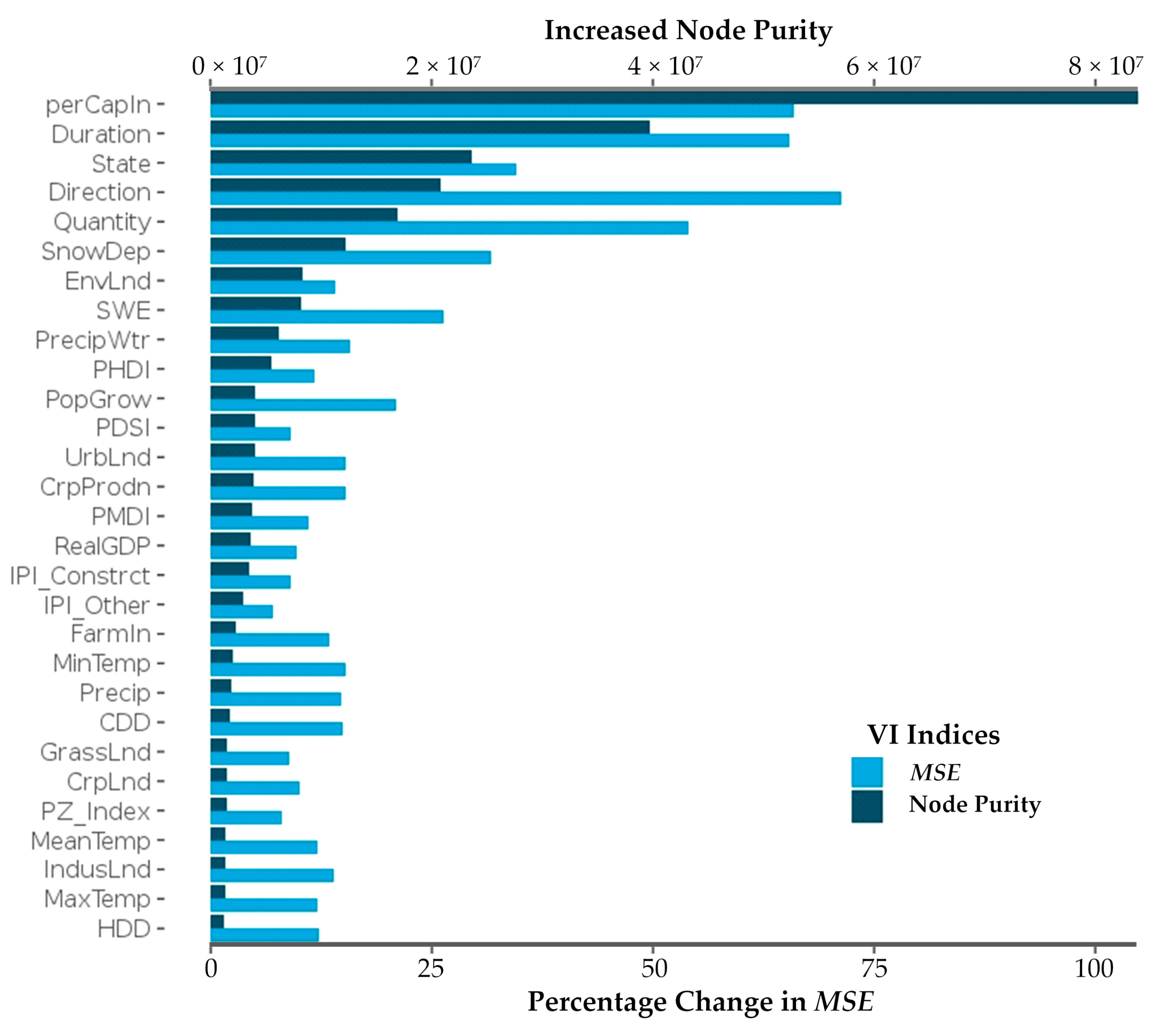
4.4. Relative Importance of Individual Variables

As discussed in Section 3.3, the importance of each influencing factor associated with water price, reflected in the contribution of their corresponding variables to the RFR models’ predictive performance, can be assessed through VI rankings. Among the considered factors, we expect that the transaction attribute variables are the dominant price determinants, particularly Direction as the price differentials across sectors in the western United States have become increasingly considerable [60]. The VI of Duration is also hypothesized to be significant since the unit price is normally higher if the transaction is a sale as compared to the lease of water rights. The variable State was used as a proxy to capture the potential state-level factors which could not be easily encapsulated in clear quantitative or categorical variables. It is thus also participated to be an important price determinant due to the facts that water institutions and state laws vary across the western states and that these factors play a key role in explaining the price disparities [10]. Furthermore, our hypothesis is that the hydrologic and the economic variables are of importance, but less important than the attribute variables. First, water scarcity as a consequence of precipitation, evaporation and temperature variations, which is reflected in the drought indices, is a major driver of water price. This has been supported by the conclusions of most studies [13,61]. Second, the correlations between economic growth (as well as the demographic factors) and the prices of natural resources in general have been statistically proven to be significant [62,63]. Land use change can shape water demands. For example the rapid urbanization witnessed in Colorado has led to a substantial number of water transfers to urban uses. But we expect the land use variables to play a relatively less important role due to their indirect impact on water price.

The VI of the predictor variables were computed and ranked based on both of the importance metrics introduced in Section 3.3 (Figure 8). Generally, it reveals that the importance scores with the PVI metric are more evenly distributed than that using the NVI metric. Importance of most of the influencing factors is consistent with our hypothesis. The top-five important variables ranked by both metrics are the same: Direction, Duration, Quantity, State, and PerCapIn, four out of which are categorized as attribute variables. In addition to the possible reasons mentioned earlier, this may also be because the values of the four attribute variables are specifically associated with each trade, which differ from other variables that used mean data values at different spatial and time scales. As a result, values of the attribute variables are more accurate and thus exhibit higher predictive strength.

Among the four most important attribute variables, Direction has the strongest predictive power according to PVI ranking (△MSE ≈ 75%). This is consistent with our hypothesis as Direction is categorized by the types of buyers and sellers, which directly reflect the difference in marginal value between prior and posterior water uses, thus should be a substantial factor in determining price. In general, environmental buyers pay lower prices than agricultural and urban buyers. This may be due to the fact that environmental use purchases are usually made by federal or state agencies that have monopsony power, especially since many transferred water rights are used for mandated ecological protection [5]. Urban purchasers usually are more willing to pay higher prices than agricultural buyers as the marginal value of water for industrial and commercial sectors is higher than that of agricultural use. Furthermore, municipal water supply is very vulnerable to water shortage, consequently, more likely to cost a premium to acquire a high level of water reliability [64].

Duration also makes a large contribution when used to predict water transfer price. It is the second important variable according to both VI rankings. This is also what we expected. Generally, price per committed volume of water sales is greater than that of leases due to the essential difference of using water rights in perpetuity versus only for a finite duration. This may also be due to the premium paid for permanent water rights in the study area over recent decades [65]. Moreover, unlike water lease, whose physical water transfer and negotiations are close in time, water sale often involves a longer and relatively complex process, resulting in higher transaction costs.

Although it has been frequently reported that the price of water transfer and the volume of water being traded are correlated [12,61,66], the influence of Quantity according to PVI ranking is much stronger than our anticipation. This may be a response to the economics of scale phenomenon in trade. That is, transaction cost per unit volume of water decreases as traded water volume increases. Consequently, water price falls as transactions involve greater size of water, which has been discussed in previous studies [12,66,67]. This result also indicates that the proxy variable State was very important as hypothesized, which implies that the price variation between states may largely be due to their differences in factors such as state laws, institutional arrangements and major water projects. We therefore suggest that some more complicated variables can be designed to replace the State variable in future studies. For example, a binomial variable can be used to represent whether the water market in a state tend to facilitate water transfer, as laws in some states were designed to expedite transactions that consequently reduced transaction costs and price [48,65].

Interestingly, while most of the economic and demographic variables only show moderate importance, PerCapIn exhibits significant impact on water price according to both VI rankings. This is out of our expectation. Particularly, the variable PerCapIn alone contributes to nearly one third of the total node purity generated by all 29 variables based on the NVI metric. The change in the state population was also expected to be a major driving force for water demand and thus for price, but PopGrow is only ranked 8th and 11th by the PVI and NVI metrics, respectively. This implies that the population growth itself may not be a dominant factor on water price, but the price may increase as the population becomes wealthier. This result is consistent with previous findings in Brookshire et al. [5].

SnowDep and SEW demonstrate high predictability according to both VI rankings. This may be due to the fact that the seasonal phase of snow storage plays a critical role in freshwater supply in the western states. In a recent study, it was found that 53% of the total runoff in the western states originates as snowmelt, despite only 37% of the precipitation falling as snow [68]. However, our result reveals that other meteorological and hydrologic variables only contribute low to moderate contributions in predicting water price. This may be because the use of state-level data for these variables is inappropriate as the states’ boarders are usually larger than the breadth of water markets. The land use variables were also expected to influence the water price as they reflect the change of water use in both buyer and seller sides. The NVI ranking shows that the change of urban and environmental land use is greater than that of agriculture land use. We therefore conclude that the demand of buyer sides dominates the water price because municipal and environmental water users are the largest water purchasers in the study region. One should note the VI of each variable only reflects its degree of predictive power and how strong it is correlated with the response variable, and it does not necessarily infer strong causation between the predictors and water price. Nevertheless, the VI rankings are still useful tools for factor importance analysis.

5. Conclusions and Suggestions

In many water markets, uncertainty of asking and offering prices due to the complex relationship between water price and its associated influencing factors is a major obstacle for participants in making efficient decisions. Improved water price prediction and better understanding of price determination have become more important in facing this challenge [8,9]. Recently, with the advances in big data analysis and computer sciences, it has become possible to explore the applications of machine learning algorithms in water rights price prediction. This paper, for the first time, proposed three RFR-based models to predict the price of water rights transfer. The conclusions and suggestions are as follows:

(1)

Despite the large price variance (the CoV of water price is over 214% in this study) and different market structures (i.e., the ratio between leases and sales) across the western states, the RFR models showed good predictive capability for water price while producing plausible VI rankings. This demonstrates the great potential of the RFR algorithm in capturing the complex and nonlinear relationships between water price and a large number of determinants that the traditional regression modeling often fails to address adequately. The RFR models are also able to include many correlated variables, whereas adding to many correlated variables can cause the serious issue of multicollinearity in traditional regression modeling. Moreover, the RFR models not only beat the DT baseline model, but also avoided overfitting, which the baseline model suffered from in the generalization process.

(2)

The BVE procedure can improve the overall model accuracy to some degree, which reflects the advantage of filtering out variables with low to moderate VI. However, the improvement was not significant as the RFR algorithm is robust to including low informative variables. Despite the algorithm’s ability to handle noisy variables, we do not suggest using as many predictor variables as possible for RFR modeling. The pre-selection of variables with hypothesized pertinence to water rights price, based on the researchers’ knowledge and data availability, is an essential part of RFR modeling. Potential predictor variables such as seniority and quality of water rights, water storage, water consumption, prices of relevant commodities, etc. can also be taken into account for future studies.

(3)

There remain a few limitations in this paper. First, The RFR models may result in higher predictive power if trained with finer spatial resolution data (e.g., county or sub-basin levels), particularly for those variables that have high spatial variations within states. But because we were not able to acquire the precise geographic locations of each transaction, the dataset assembled for this study lacked specificity to some degree. Second, many informal transactions, of which the price can be determined by different factors, were not recorded by the Water Strategist [10]. Nevertheless, the recorded water trade data still allowed us to conduct empirical analysis about state-level impacts on water price. Another minor limitation of this study is the assumption on the optimal latency of the hydrologic variables, of which the lagging information with longer or shorter periods may improve the predictive performances of the models. However, as it is beyond the scope of this paper, we suggest separate studies be conducted in examining the optimal lag-time of these predictors for water price prediction.

(4)

As water markets are heterogeneous, future studies, using the RFR-based models, focusing on price prediction for specific regional or local water markets are suggested, which can generate more valuable price information at lower scales. With continued data acquisition, the models presented in this study can be further improved and commercialized for use of water market participants in making water trade decisions, water administrators in water management or policy makers in policy implication analysis, and could ultimately make a contribution to higher economic and water use efficiency.

References

1. Grafton, R.Q.; Libecap, G.; McGlennon, S.; Landry, C.; O’Brien, B. An Integrated Assessment of Water Markets: A Cross-Country Comparison. Rev. Environ. Econ. Policy 2011, 5, 219–239. [Google Scholar] [CrossRef]
2. Deng, X.; Song, X.; Xu, Z. Transaction Costs, Modes, and Scales from Agricultural to Industrial Water Rights Trading in an Inland River Basin, Northwest China. Water 2018, 10, 1598. [Google Scholar] [CrossRef]
3. Qureshi, M.E.; Whitten, S.M.; Mainuddin, M.; Marvanek, S.; Elmahdi, A. A biophysical and economic model of agriculture and water in the Murray-Darling Basin, Australia. Environ. Model. Softw. 2013, 41, 98–106. [Google Scholar] [CrossRef]
4. Skurray, J.H.; Roberts, E.J.; Pannell, D.J. Hydrological challenges to groundwater trading: Lessons from south-west Western Australia. J. Hydrol. 2012, 412–413, 256–268. [Google Scholar] [CrossRef]
5. Brookshire, D.S.; Colby, B.; Ewers, M.; Ganderton, P.T. Market prices for water in the semiarid West of the United States. Water Resour. Res. 2004, 40, W4S–W9S. [Google Scholar] [CrossRef]
6. Brooks, R.; Harris, E. Efficiency gains from water markets: Empirical analysis of Watermove in Australia. Agric. Water Manag. 2008, 95, 391–399. [Google Scholar] [CrossRef]
7. Chong, H.; Sunding, D. Water Markets and Trading. Annu. Rev. Env. Resour. 2006, 31, 239–264. [Google Scholar] [CrossRef]
8. Anderson, T.L.; Scarborough, B.; Watson, L.R. Tapping Water Markets, 1st ed.; Routledge: New York, NY, USA, 2012; pp. 1–9. ISBN 978-1617261008. [Google Scholar]
9. Nguyen-Ky, T.; Mushtaq, S.; Loch, A.; Reardon-Smith, K.; An-Vo, D.A.; Ngo-Cong, D.; Tran-Cong, T. Predicting water allocation trade prices using a hybrid Artificial Neural Network-Bayesian modelling approach. J. Hydrol. 2017. [Google Scholar] [CrossRef]
10. Edwards, E.C.; Libecap, G.D. Water Institutions and the Law of One Price. In Handbook on the Economics of Natural Resources; Edward Elgar Publishing: Cheltenham, UK, 2015; pp. 442–473. [Google Scholar]
11. De Mouche, L.; Landfair, S.; Ward, F.A. Water Right Prices in the Rio Grande: Analysis and Policy Implications. Int. J. Water Resour. Dev. 2011, 27, 291–314. [Google Scholar] [CrossRef]
12. Payne, M.T.; Smith, M.G.; Landry, C.J. Price Determination and Efficiency in the Market for South Platte Basin Ditch Company Shares. J. Am. Water Resour. Assoc. 2014, 50, 1488–1500. [Google Scholar] [CrossRef]
13. Bjornlund, H.; Rossini, P. Fundamentals Determining Prices and Activities in the Market for Water Allocations. Int. J. Water Resour. Dev. 2005, 21, 355–369. [Google Scholar] [CrossRef]
14. Bjornlund, H.; Rossini, P. Fundamentals Determining Prices in the Market for Water Entitlements: An Australian Case Study. Int. J. Water Resour. Dev. 2007, 23, 537–553. [Google Scholar] [CrossRef]
15. Brennan, D. Price formation on the Northern Victorian water exchange. In Proceedings of the 48th Conference of the Australian Agricultural and Resource Economics Society, Melbourne, Australia, 11–12 February 2004. [Google Scholar]
16. Brown, T.C. Trends in water market activity and price in the western United States. Water Resour. Res. 2006, 42, W9402. [Google Scholar] [CrossRef]
17. Li, X.; Maier, H.R.; Zecchin, A.C. Improved PMI-based input variable selection approach for artificial neural network and other data driven environmental and water resource models. Environ. Model. Softw. 2015, 65, 15–29. [Google Scholar] [CrossRef]
18. Maier, H.R.; Jain, A.; Dandy, G.C.; Sudheer, K.P. Methods used for the development of neural networks for the prediction of water resource variables in river systems: Current status and future directions. Environ. Model. Softw. 2010, 25, 891–909. [Google Scholar] [CrossRef]
19. Yang, T.; Asanjan, A.A.; Welles, E.; Gao, X.; Sorooshian, S.; Liu, X. Developing reservoir monthly inflow forecasts using Artificial Intelligence and Climate Phenomenon Information. Water Resour. Res. 2017, 53, WR020482. [Google Scholar] [CrossRef]
20. Khan, S.; Dassanayake, D.; Mushtaq, S.; Hanjra, M.A. Predicting water allocations and trading prices to assist water markets. Irrig. Drain. 2010, 59, 388–403. [Google Scholar] [CrossRef]
21. Panchal, G.; Ganatra, A.; Shah, P.; Panchal, D. Determination of Over-Learning and Over-Fitting Problem in Back Propagation Neurl Network. Int. J. Soft Comput. 2011, 2, 40–51. [Google Scholar] [CrossRef]
22. Srivastava, N.; Hinton, G.; Krizhevsky, A.; Sutskever, I.; Salakhutdinov, R. Dropout: A Simple Way to Prevent Neural Networks from Overfitting. J. Mach. Learn. Res. 2014, 15, 1929–1958. [Google Scholar]
23. Breiman, L. Random Forests. Mach. Learn. 2001, 45, 5–32. [Google Scholar] [CrossRef]
24. Cavallo, D.P.; Cefola, M.; Pace, B.; Logrieco, A.F.; Attolico, G. Contactless and non-destructive chlorophyll content prediction by random forest regression: A case study on fresh-cut rocket leaves. Comput. Electron. Agric. 2017, 140, 303–310. [Google Scholar] [CrossRef]
25. Booth, A.; Gerding, E.; Mcgroarty, F. Automated trading with performance weighted random forests and seasonality. Expert Syst. Appl. 2014, 41, 3651–3661. [Google Scholar] [CrossRef]
26. Ballings, M.; Van den Poel, D.; Hespeels, N.; Gryp, R. Evaluating multiple classifiers for stock price direction prediction. Expert Syst. Appl. 2015, 42, 7046–7056. [Google Scholar] [CrossRef]
27. Zhang, J.; Cui, S.; Xu, Y.; Li, Q.; Li, T. A novel data-driven stock price trend prediction system. Expert Syst. Appl. 2018, 97, 60–69. [Google Scholar] [CrossRef]
28. Liu, D.; Li, Z. Gold Price Forecasting and Related Influence Factors Analysis Based on Random Forest. In Proceedings of the Tenth International Conference on Management Science and Engineering Management, Baku, Azerbaijan, 30 August–4 September 2016. [Google Scholar] [CrossRef]
29. Liu, C.; Hu, Z.; Li, Y.; Liu, S. Forecasting copper prices by decision tree learning. Resour. Policy 2017, 52, 427–434. [Google Scholar] [CrossRef]
30. Gaillard, P.; Goude, Y.; Nedellec, R. Additive models and robust aggregation for GEFCom2014 probabilistic electric load and electricity price forecasting. Int. J. Forecast. 2016, 32, 1038–1050. [Google Scholar] [CrossRef]
31. Chen, F.; Howard, H. An alternative model for the analysis of detecting electronic industries earnings management using stepwise regression, random forest, and decision tree. Soft Comput. 2016, 20, 1945–1960. [Google Scholar] [CrossRef]
32. Antipov, E.A.; Pokryshevskaya, E.B. Mass appraisal of residential apartments: An application of Random forest for valuation and a CART-based approach for model diagnostics. Expert Syst. Appl. 2012, 39, 1772–1778. [Google Scholar] [CrossRef]
33. Lessmann, S.; Voß, S. Car resale price forecasting: The impact of regression method, private information, and heterogeneity on forecast accuracy. Int. J. Forecast. 2017, 33, 864–877. [Google Scholar] [CrossRef]
34. Yang, T.; Gao, X.; Sorooshian, S.; Li, X. Simulating California reservoir operation using the classification and regression-tree algorithm combined with a shuffled cross-validation scheme. Water Resour. Res. 2016, 52, 1626–1651. [Google Scholar] [CrossRef]
35. He, X.; Zhao, T.; Yang, D. Prediction of monthly inflow to the Danjiangkou reservoir by distributed hydrological model and hydro-climatic teleconnections. J. Hydroelectr. Eng. 2013, 32, 4–9. [Google Scholar]
36. Papacharalampous, G.; Tyralis, H. Evaluation of random forests and Prophet for daily streamflow forecasting. Adv. Geosci. 2018, 45, 201–208. [Google Scholar] [CrossRef]
37. Herrera, M.; Torgo, L.; Izquierdo, J.; Pérez-García, R. Predictive models for forecasting hourly urban water demand. J. Hydrol. 2010, 387, 141–150. [Google Scholar] [CrossRef]
38. Chen, G.; Long, T.; Xiong, J.; Bai, Y. Multiple Random Forests Modelling for Urban Water Consumption Forecasting. Water Resour. Manag. 2017, 31, 4715–4729. [Google Scholar] [CrossRef]
39. Feng, Q.; Liu, J.; Gong, J. Urban Flood Mapping Based on Unmanned Aerial Vehicle Remote Sensing and Random Forest Classifier—A Case of Yuyao, China. Water 2015, 7, 1437–1455. [Google Scholar] [CrossRef]
40. Muñoz, P.; Orellana-Alvear, J.; Willems, P.; Célleri, R. Flash-Flood Forecasting in an Andean Mountain Catchment—Development of a Step-Wise Methodology Based on the Random Forest Algorithm. Water 2018, 10, 1519. [Google Scholar] [CrossRef]
41. Wu, J.; Chen, Y.F.; Yu, S.N. Research on drought prediction based on random forest model. China Rural Water Hydropower 2016, 17, 17–22. [Google Scholar]
42. Eccel, E.; Ghielmi, L.; Granitto, P.; Barbiero, R.; Grazzini, F.; Cesari, D. Prediction of minimum temperatures in an alpine region by linear and non-linear post-processing of meteorological models. Nonlinear Process. Geophys. 2007, 14, 211–222. [Google Scholar] [CrossRef]
43. Karthick, S.; Malathi, D.; Arun, C. Weather prediction analysis using random forest algorithm. Int. J. Pure Appl. Math. 2018, 118, 255–262. [Google Scholar]
44. Ibarra-Berastegi, G.; Saénz, J.; Ezcurra, A.; Elías, A.; Diaz Argandoña, J.; Errasti, I. Downscaling of surface moisture flux and precipitation in the Ebro Valley (Spain) using analogues and analogues followed by random forests and multiple linear regression. Hydrol. Earth Syst. Sci. 2011, 15, 1895–1907. [Google Scholar] [CrossRef]
45. He, X.; Chaney, N.W.; Schleiss, M.; Sheffield, J. Spatial downscaling of precipitation using adaptable random forests. Water Resour. Res. 2016, 52, 8217–8237. [Google Scholar] [CrossRef]
46. Brewer, J.; Glennon, R.; Ker, A.; Libecap, G.D. Water markets in the west: Prices, trading and contractual form. Econ. Inq. 2008, 46, 91–112. [Google Scholar] [CrossRef]
47. Donohew, Z. Property rights and western United States water markets. Aust. J. Agric. Resour. Econ. 2009, 53, 85–103. [Google Scholar] [CrossRef]
48. Hansen, K.; Howitt, R.; Williams, J. An Econometric Test of Water Market Structure in the Western United States. Nat. Resour. J. 2015, 55, 127–152. [Google Scholar]
49. Ho, T.K. Random decision forests. In Proceedings of the 3rd International Conference on Document Analysis and Recognition, Montreal, QC, Canada, 14–16 August 1995. [Google Scholar] [CrossRef]
50. Zhong, S.; Xie, X.; Lin, L. Two-layer random forests model for case reuse in case-based reasoning. Expert Syst. Appl. 2015, 42, 9412–9425. [Google Scholar] [CrossRef]
51. Liaw, A.; Wiener, M. Classification and Regression by randomForest. R News 2002, 2, 18–22. [Google Scholar]
52. Hjerpe, A. Computing Random Forests Variable Importance Measures (VIM) on Mixed Continuous and Categorical Data. Master’s Thesis, KTH Royal Institute of Technology, Stockholm, Sweden, 2016. [Google Scholar]
53. Fox, E.W.; Hill, R.A.; Leibowitz, S.G.; Olsen, A.R.; Thornbrugh, D.J.; Weber, M.H. Assessing the accuracy and stability of variable selection methods for random forest modeling in ecology. Environ. Monit. Assess. 2017, 189, 316. [Google Scholar] [CrossRef]
54. Lujan-Moreno, G.A.; Howard, P.R.; Rojas, O.G.; Montgomery, D.C. Design of experiments and response surface methodology to tune machine learning hyperparameters, with a random forest case-study. Expert Syst. Appl. 2018, 109, 195–205. [Google Scholar] [CrossRef]
55. Bernard, S.; Heutte, L.; Adam, S. Influence of Hyperparameters on Random Forest Accuracy. In Proceedings of the 8th International Workshop, MCS 2009, Reykjavik, Iceland, 10–12 June 2009. [Google Scholar] [CrossRef]
56. Yang, T.; Asanjan, A.A.; Faridzad, M.; Hayatbini, N.; Gao, X. An enhanced artificial neural network with a shuffled complex evolutionary global optimization with principal component analysis. Inform. Sci. 2017, 418–419, 302–316. [Google Scholar] [CrossRef]
57. Biau, G. Analysis of a Random Forests Model. J. Mach. Learn. Res. 2010, 13, 1063–1095. [Google Scholar]
58. Piñeiro, G.; Perelman, S.; Guerschman, J.P.; Paruelo, J.M. How to evaluate models: Observed vs. predicted or predicted vs. observed? Ecol. Model. 2008, 216, 316–322. [Google Scholar] [CrossRef]
59. Goodfellow, I.; Bengio, Y.; Courville, A.; Bengio, Y. Deep Learning, 1st ed.; MIT Press: Cambridge, MA, USA, 2016; ISBN 9780262035613. [Google Scholar]
60. Libecap, G.D. Institutional path dependence in climate adaptation: Coman’s some unsettled problems of irrigation. Am. Econ. Rev. 2011, 101, 64–80. [Google Scholar] [CrossRef]
61. Ghosh, S. Droughts and water trading in the western United States: Recent economic evidence. Int. J. Water Resour. Dev. 2018, 35, 145–159. [Google Scholar] [CrossRef]
62. Mideksa, T.K. The economic impact of natural resources. J. Environ. Econ. Manag. 2013, 65, 277–289. [Google Scholar] [CrossRef]
63. Mehrara, M.; Baghbanpour, J. Analysis of the Relationship between Total Natural Resources Rent and Economic Growth: The Case of Iran and MENA Countries. Int. J. Appl. Econ. Stud. 2015, 3, 1–7. [Google Scholar]
64. Lach, D.; Ingram, H.; Rayner, S. Maintaining the status quo: How institutional norms and practices create conservative water organizations. Texas Law Rev. 2005, 83, 2027–2053. [Google Scholar]
65. Grafton, R.Q.; Libecap, G.D.; Edwards, E.C.; O’Brien, R.B.; Landry, C. Comparative assessment of water markets: Insights from the Murray–Darling Basin of Australia and the Western USA. Water Policy 2012, 14, 175–193. [Google Scholar] [CrossRef]
66. Payne, M.T.; Smith, M.G. Price determination and efficiency in the market for water rights in New Mexico’s Middle Rio Grande Basin. Int. J. Water Resour. Dev. 2013, 29, 588–604. [Google Scholar] [CrossRef]
67. Colby, B.G.; Crandall, K.; Bush, D.B. Water Right Transactions: Market Values and Price Dispersion. Water Resour. Res. 1993, 29, 1565–1572. [Google Scholar] [CrossRef]
68. Li, D.; Wrzesien, M.L.; Durand, M.; Adam, J.; Lettenmaier, D.P. How much runoff originates as snow in the western United States, and how will that change in the future? Geophys. Res. Lett. 2017, 44, 6163–6172. [Google Scholar] [CrossRef]
Figure 1. Total committed water quantity traded and numbers of transactions for each western state in the study area (Water Strategist, 1987–2009).
Water 11 00228 g001
Figure 2. Schematic of the random forest regression algorithm based on the Bagging (Bootstrap Aggregating) method.
Water 11 00228 g002
Figure 3. Schematic of the backward variable elimination (BVE) procedure for model selection. The count variable i denotes the round number of model training. It is reset to 1 before entering the reduced RFR selection cycle. The variable f denotes the number of variable(s) discarded. R is the number of runs. The variable importance scores are obtained simultaneously when a RFR-full is trained each time.
Water 11 00228 g003
Figure 4. Pearson correlation coefficient (PCC) versus number of predictor variables at each step of the backward elimination procedure. The PCC values in each panel are averaged values over multiple runs; they are between the actual water prices and predicted water prices generated by reduced RFR models as variables are removed stepwise. The vertical dash lines denote the reduced models that produce the highest PCC values. Panel (a) refers to the procedure using node impurity based VI ranking and Panel (b) refers to the procedure using permutation based VI ranking.
Water 11 00228 g004
Figure 5. Center-log normalized out-of-bag (OOB) error curves for models with different hyperparameter configurations. To better illustrate the figure, all of the normalized errors were scaled using the equation y = ln(err − 0.5). Panel (ad), (eh) and (il) correspond to the RFR-full, RFR-red-P and RFR-red-N, respectively. The percentages on top of each column are the percentages of total number of variables that are available for splitting at each tree node. Curves in different colors represent different minimal size of leaf nodes.
Water 11 00228 g005
Figure 6. Jitter boxplots of predictive accuracies from 8 repetitions of 10-fold cross-validation. Each jitter point represents accuracy for one of the 80 validation rounds. Panel (a) and Panel (b) are predictive accuracies in terms of Pearson correlation coefficient and normalized root mean squared error, respectively. The triangles in each box represent the means of the model performances.
Water 11 00228 g006
Figure 7. A set of examples for actual vs. predicted price scatterplots in one round of cross-validation. Panel (a,d), (b,e) and (c,f) correspond to the RFR-full, RFR-red-N and RFR-red-P models, respectively. Panel (ac) represent the cross validation rounds with the poorest accuracy for each model, Panel (df) represent the cross validation rounds that have the highest accuracy for each model. The green dash lines in each panel are the 1-1 lines. The red solid lines in each panel are the best fit lines between actual and predicted water prices. The corresponding regression equations and Pearson correlation coefficients are given in each panel.
Water 11 00228 g007
Figure 8. Variable importance rankings for all predictor variables averaged through multiple runs. The dark blue bars represent the decreased node impurities as each variable is used for partitioning; the light blue bars represent the percentage change in mean squared errors of model prediction before and after permuting each variable. The variable names on the vertical axis are ranked by their decreased node impurities in descending order.
Water 11 00228 g008