Abstract
In this paper, to interpret the cost structure of decentralized wastewater treatment plants (DWWTPs) in rural regions, a simple nonparametric regression algorithm known as multivariate adaptive regression spline (MARS) was proposed and applied to simulate the construction cost (CC), operation and maintenance cost (OMC), and total cost (TC). The effects of design treatment capacity (DTC), removal efficiency of chemical oxygen demand (RCOD), and removal efficiency of ammonia nitrogen (RNH3-N) on the cost functions of CC, OMC, and TC were analyzed in detail. The results indicated that: (1) DTC is the most important parameter to determine cost structure with relative importance of 100%, followed by RCOD and RNH3-N with relative importance of 16.55%, and 9.75%, respectively; (2) when DTC is less than 5 m3/d, the slopes of CC and TC on DTC are constants of 1.923 and 1.809, respectively, with no relationship with RCOD and RNH3-N; (3) when DTC is less than 20 m3/d, the OMC is a constant of 435 RMB/year; and (4) in other cases, CC, OMC, and TC are related to RCOD and RNH3-N besides DTC. Compared with widely used support vector machine (SVM) models and multiple linear regression (MLR) models, the MARS model has better statistical significance with greater R values and smaller RMSE and MAPE values, which indicated that the MARS model is a better way to approximate the cost for DWWTPs.
1. Introduction
“New rural construction” proposed in 2005 in China, is a new policy to realize sustainable development in rural regions with a prosperous economy, perfect facilities, a beautiful environment, and a harmonious civilization [1,2]. However, increasing amount of domestic sewage was drained into rural water environment without proper treatment. To construct “new rural”, economic and effective sewage treatment facilities are needed [3]. In rural regions with limited budgets, the cost structure of wastewater treatment including construction cost (CC), operating and maintenance cost (OMC), and total cost (TC) require better understanding to help create economically feasible water quality management programs in the future, and to help in the planning of wastewater treatment plants [4,5,6].
In the past, cost structures of municipal wastewater treatment plants (MWWTPs) were studied in lots of literatures, and wastewater treatment capacity was the primary consideration. Regression methods, such as simple linear regression, multiple linear regression, non-linear regression were applied to evaluate the relationship between treatment capacity and treatment cost [4,7]. Since uncertainties exist in cost estimations, such as wastewater generation, treatment, and reuse, fuzzy technology was integrated into regression models to generate fuzzy linear regression models, fuzzy nonlinear regression models, and fuzzy goal regression models. The input and output variables and regression coefficients were taken as fuzzy numbers in fuzzy regression models [4,7,8,9,10]. The effects of treatment level (secondary treatment and advanced secondary treatment) or treatment units (anaerobic pond, anaerobic tank, constructed wetland) combined with treatment capacity on CC and OMC of MWWTPs were also analyzed and modeled [7,8,9,11]. In rural regions, the CC and OMC of wastewater treatment plants (WWTPs) are higher than urban regions due to a smaller and dispersed population, intermittent sewage discharge, lower water supply standard, significant fluctuation of water consumption, smaller sewage treatment scale, more complex topographic conditions, and more difficult to collect wastewater. To decrease CC and OMC of WWTPs in rural regions, the decentralized wastewater treatment plants (DWWTPs), which means that sewage is collected according to the zoning and the sewage is treated separately in each zone, are suitable. Therefore, DWWTPs are drawing wider interest from all over the world, especially water-deficient countries and regions [12,13]. However, only treatment capacity is given to the cost structure of DWWTPs [12,13,14]. In MWWTPs, it was reported that removal of biological oxygen demand (BOD) and nutrients affects the cost significantly due to the substantial increase of tank volume for nitrification [15]. In this paper, the effects of removal of organic pollutants and nutrients on the cost of DWWTPs were analyzed by proposing a multivariate adaptive regression spline (MARS) model. By partitioning training data sets into separate piecewise linear segments (splines) of differing gradients (slopes), a MARS model fit the relationship between a set of input variables and dependent variables in high-dimensional data [16], which has been successfully applied to predict and classify in many engineering fields [17,18,19,20,21]. The MARS model has the advantages of suitable for nonlinear systems, easy to interpret, and variables appear in the resulting model directly. Additionally, MARS does not need to assume the distribution of the predictor variables, which is very important because the variables in cost models are not normally distributed [20]. However, MARS has not been applied to predict wastewater treatment costs to date.
In this paper, the MARS model was applied to predict CC, OMC, and TC for DWWTPs in rural regions, which can help analyze cost-efficiency more accurately. In the MARS model, factors taken into account included not only the design treatment capacity (DTC), but also the removal efficiency (R) of chemical oxygen demand (COD) and ammonia nitrogen (NH3-N), termed as RCOD and RNH3-N, respectively.
2. Methods
2.1. Data Set
The cost data for rural sewage treatment systems were collected from 215 sets of DWWTPs located in Changshu region of Jiangsu Province in China, which were in operation. The research scope included 11 districts: Bixi District, Southeast Street, Yushan Town, Meili Town, Haiyu Town, Guli Town, Shajiabang Town, Zhitang Town, Dongbang Town, Shanghu Town, and Xinzhuang Town. Since rural wastewater has the characteristic of fair biological treatability without toxic or harmful substances, four treatment technologies were adopted: membrane bioreactor (MBR), sequencing batch reactor (SBR), biological filter and artificial wetland (BFAW), and purification tank (PT). In the cost model of MWWTPs, treatment capacity and treatment level are regarded as two most important drivers [8,22]. However, in rural regions, the sewage is primarily consisted of domestic wastewater, in which COD and NH3-N are the main pollution factors [23]. Therefore, RCOD and RNH3-N were selected to represent treatment level. The mean values of parameters with various treatment capacities are shown in Table 1.

Table 1.
Mean value of parameters for the selected samples.
In Table 1, x1 refers to DTC (ranges from 1 m3/d to 110 m3/d), x2 stands for RCOD, x3 represents RNH3-N, y is TC including y1 (CC) and y2 (OMC). In this paper, CC and OMC refer to annual construction cost, and annual operation and maintenance cost, respectively. The annual construction cost is obtained using Equation (1):
where IC is the investment cost (104 RMB); r is the discount rate, which is set to be 0.035; and t is the expected life of the plant, which is assumed to be 10 years.
The construction costs were supplied by the Construction Bureau in Changshu City, and the operation and maintenance costs were supplied by Suzhou Hongyu Wastewater Treatment Engineering Limited Corporation. In the MARS model, the dataset was divided into two subsets: a training set with 160 samples for developing the MARS model and a testing set with 55 samples for verifying the developed MARS model. The training set included 88 sets with DTC of 1 m3/d, 9 sets with DTC of 2 m3/d, 21 sets with DTC of 5 m3/d, 23 sets with DTC of 10 m3/d, 7 sets with DTC of 15 m3/d, 5 sets with DTC of 20 m3/d, 2 sets with DTC of 45 m3/d, 2 sets with DTC of 50 m3/d, 2 sets with DTC of 60 m3/d, and 1 set with DTC of 110 m3/d. The other data were selected for the testing set.
The data were normalized between 0 and 1 by Equation (2) as follows:
where dnorm is the normalized value of the dataset, is the input/output variable, dmin is the minimum value of the dataset, and dmax is the maximum value of the dataset. In the following discussion, if there is no special explanation, all the variables refer to the variables being normalized.
2.2. Multivariate Adaptive Regression Spline (MARS)
Multivariate adaptive regression spline (MARS) was introduced by Friedman, which is a nonparametric regression modeling procedure that can approximate the relationship between a dependent variable (y) and a set of independent variables (x1, x2, …, xn) with a piecewise regression [16,19,23,24]. Functions fitted in piecewise regression are called basis functions (BFs) of the MARS methods. BFs can be either single spline function or a product of two or more spline functions for different explanatory variables [19,20,24,25,26,27,28,29,30]. The form of MARS is expressed based on multivariate spline basis functions as follows:
where represents the predicted value of the response; is the constant; is the coefficient of the mth term of the basis function Bm(X); M is the number of basis functions; ; is the explanatory variables associated with the basis function , i.e., the values of the jth explanatory variables at the ith node of the mth basic function; is the level of interaction between j(i,m) variables; and indicates the node locations for , which are the interface points between pieces, called knots in the MARS model. In this paper, and .
The definition of each BF is selected from the collection C where:
Each basis function is piecewise linear with a knot t at , which can be multiplied together to form non-linear functions. The location and number of the needed spline basis functions were found through a second-order forward/backward stepwise regression procedure. For example, a two-sided basis function with knot t of 0.5 is shown in Figure 1.
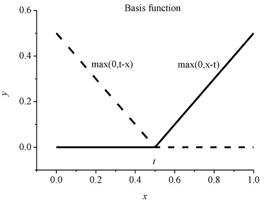
Figure 1.
A graphical representation of a spline basis function: The left spline (max (0, t −x)) is shown as a dashed line and the right spline (max (0, x − t)) is shown as a solid line.
The basis functions are generated through two steps, which are the forward phase and backward pruning phase, detailed as follows.
2.3. Step 1 (Forward Phase)
In the forward stage, MARS becomes larger by considering a great number of basis functions and all possible variables among the predictor variables. In this phase, potential knots are continuously found to be added into basis functions to improve the performance until the model reaches a predetermined allowable maximum number of basis functions. Consequently, an over-fit model is generated as follows:
where is the predicted value for the response variable.
The regression coefficients are estimated using the MARS method to obtain the center of the dependent variable.
2.4.Step 2 (Backward Pruning Phase)
In this phase, the basis function with the least contribution to the model performance was deleted one by one, leading to a simplified and generalized MARS model. Generalized cross-validation (GCV) criterion is used to assess the importance of variables, which can be expressed as follows:
in which N is the number of observations, and is the predicted values of the MARS model. is a complexity penalty that increases with number of basis functions in the model, defined as:
where M is the number of basis functions, and d is the penalizing parameter. With the rise of the d value, fewer knots are obtained and function estimation becomes smoother. The optimal value of d is among 2 to 4 [16,29]. In this study, a default value of 3 is assigned to the penalizing parameter.
The importance of the variable can be obtained by assessing the decrease in the GCV values when the variable is removed from the model. The most important variable with the highest decrease in the GCV values is assigned a score of 100. The scores of the other variables are obtained according to the ratio of the decrease in the GCV values by these variables to that of the most important variable.
The effect of the input variables on the output variables can be explained well using analysis of variance (ANOVA) decomposition of the calculation results. In this paper, the relative importance of the input variabls x1, x2, and x3 to the output variables y, y1, and y2 can be identified using ANOVA decomposition. The ANOVA decomposition of the developed MARS model is given by Equation (8) as follows:
where is the overall basis function involving only a single variable, is the overall basis function involving exactly two variables, and is the overall basis function involving three variables. The MARS model is created using the Software Salford Predictive Modeler 8.2, Salford Systems Company, San Diego, U.S.
3. Results and Discussion
3.1. Choose the Maximum Basis Function Number and Order Number
The maximum basis function number determined the performance of the MARS model in the forward step. The effects of numbers of maximum basis functions on the training performance are significantly different for model order in the MARS model, shown in Figure 2. Model order refers to the maximum interaction number of the basis functions.
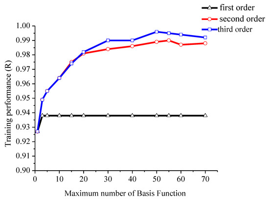
Figure 2.
Effect of maximum number of basis functions as well as order on model performance R based on the training set of y.
The training performance was assessed in terms of coefficient R. The value of R was determined using Equation (9) as follows:
where and are the actual and predicted values, respectively, and and are the means of actual and predicted values corresponding to n patterns. In this study, the value of n was 160 and 55 for the training and testing datasets, respectively.
It can be shown from Figure 2 that for the first order curve, the training performance increased with the maximum basis function number initially, and then remained invariable when the maximum basis function number was greater than 5, which means that the maximum basis function number can be chosen to be greater than 5. For the second order curve and the third order curve, we found that the two curves kept the same variation trend when the maximum basis function number was lower than 20. When the maximum basis function number was greater than 20, the third order training performance curve was better than that of the second order. However, the advantage was not apparent. The coefficient R was 0.981 with a maximum basis function number of 20 for the second order, which was close to 1. Consequently, to simplify the MARS model, model order was set to be 2, and the maximum basis function number was set to be 20. The input and output datasets were normalized using Equation (2).
3.2. Basis Functions and ANOVA Decomposition
3.2.1. Construction Cost (CC)
Through the forward phase and backward pruning phase, six basis functions were used to reach the minimum GCV value, which can represent the construction cost (CC) with the best solution. The MARS expression of CC (y1) was given according to Equation (10) and Table 2:
Table 2.
Basis functions of y1 and corresponding coefficients.
The details of the basis functions in the MARS model for construction cost (y1) are shown in Table 2. The effects of variables x1, x2, and x3 on y1 were determined using the slopes and intervals of basis functions.
- (1)
- In Table 2, the first column Bm(x) (m = 1, 2, …, 6) refers to the basis functions in the MARS model, the second column describes the equation form for Bm(x) (m = 1, 2, …, 6), and the third column is the coefficient for Bm(x) (m = 1, 2, …, 6). For example, for B1(x) in Table 2, if (x1 − 0.037) is greater than 0, i.e., DTC greater than 5 m3/d, then the value of B1(x) is equal to (x1 − 0.037); and B1(x) is equal to 0 if (x1 − 0.037) is less than or equal to 0. A positive estimated coefficient βm for the basis function indicated an increased construction cost, and a negative estimated coefficient βm indicated a decreased construction cost. From this information, the effect of x1 on y1 had three impacts. When x1 was less than 0.037 (DTC less than 5 m3/d), then y1 (CC) had no relationship with either x2 (RCOD) or x3 (RNH3-N), and increased by 1.923 for each 1% increase in x1.
- (2)
- When x1 was greater than 0.037 and less than 0.083 (DTC greater than 5 m3/d and less than 10 m3/d), then y1 (CC) depended on both x1 and x2 (RCOD) with no relationship with x3 (RNH3-N).
- (i)
- When x2 was less than 0.716 (RCOD less than 69.5%), then y1 (CC) depended on x1 without relationship with x2, and increased by 1.19 for each 1% increase in x1.
- (ii)
- When x2 was greater than 0.716 and less than 0.746 (RCOD greater than 69.5% and less than 72.0%), then y1 (CC) had a relationship with both x1 and x2, and increased by 1.19 to 1.509 for each 1% increase in x1 corresponding to x2 values of 0.716 and 0.746, respectively. The slope of y1 increased with the increase of x2.
- (iii)
- When x2 was greater than 0.746 (RCOD greater than 72.0%), then y1 (CC) increased by 0.323 to 1.507 for each 1% increase in x1 corresponding to x2 values of 1 and 0.746, respectively. The slope of y1 decreased with the increase of x2.
In summary, when x1 was greater than 0.037 and less than 0.083 (DTC greater than 5 m3/d and less than 10 m3/d), the maximum slope of CC on DTC was a constant of 1.509.
- (3)
- When x1 was greater than 0.083 (DTC more than 10 m3/d), then y1 (CC) also depended on x1, x2 (RCOD), and x3 (RNH3-N) together, which are described in detail as follows:
- (i)
- When x2 was less than 0.716 (RCOD less than 69.5%), then y1 (CC) had a relationship with both x1 and x3 without consideration of x2, and increased by 0.253 (x3 = 0) to 1.055 (x3 = 1) for each 1% increase in x1. The effect of x1 on y1 increased with the increase of x3.
- (ii)
- When x2 was greater than 0.716 and less than 0.746 (RCOD greater than 69.5% and less than 72%), then y1 (CC) is related to x1, x2 and x3 together. With an increase of x2 and x3, the slope of y1 on x1 increased accordingly, and increased by 0.253 (corresponding to x2 = 0.716 and x3 = 0) to 1.374 (corresponding to x2 =0.746 and x3 = 1.0) for each 1% increase in x1.
- (iii)
- When x2 was greater than 0.746 (RCOD greater than 72%), then y1 (CC) was also related to x1, x2, and x3 together. However, the slope of y1 on x1 increased with the increase of x3 and the decrease of x2, and increased by −0.614 (corresponding to x2 = 1 and x3 = 0) to 1.374 (corresponding to x2 = 0.746 and x3 = 1.0) for each 1% increase in x1.
In summary, when x1 is greater than 0.083 (DTC greater than 10 m3/d), the maximum slope of CC on DTC was 1.374.
Therefore, conclusions can be drawn as follows:
- (1)
- The construction cost (CC) increased with design treatment capacity (DTC), and the maximum slope of CC on DTC decreased gradually from 1.923 to 1.374 in accordance with x1 from 0 to 1.0. The variation of slope was also determined by x2 and x3.
- (2)
- When x1 was less than 0.037 (DTC less than 5 m3/d), the slope of y1 kept a constant of 1.923, and had no relation with neither x2 (RCOD) nor x3 (RNH3-N). The result indicated that when DTC was less than 5 m3/d, the relationship between CC and DTC was linear with a coefficient of 1.923.
- (3)
- When x1 was greater than 0.037 and less than 0.083 (DTC ranged from 5 m3/d to 10 m3/d), the slope of y1 had a relationship with x1 (DTC) and x2 (RCOD) without any consideration of x3 (RNH3-N).
- (4)
- When x1 was greater than 0.083 (DTC greater than 10 m3/d) and x2 was less than 0.716 (RCOD less than 69.5%), and the slope of y1 had a relationship with DTC (x1) and RNH3-N (x3) without any consideration of RCOD (x2).
The ANOVA decomposition of the MARS model aims to put together the basis functions with the same input variables. The ANOVA decomposition of y1(CC) is shown in Table 3, from which it is clear that the variable DTC had the maximum effect on y1, which has a maximum value of GCV, indicating the importance of the corresponding ANOVA function.
Table 3.
Results of ANOVA decomposition in construction cost.
In Table 3, the ANOVA function number is listed in the first column; the second column provides the standard deviation of this function, which gives an indication of its relative importance to the overall model and can be interpreted in a manner similar to the standardized regression coefficient in a linear model; the third column also gives an indication of the importance of the corresponding ANOVA function by listing the GCV score for a model with all BFs corresponding to that particular ANOVA function removed; the fourth column gives the number of BFs comprising the ANOVA function; and the last column gives the particular input variables associated with the ANOVA function.
3.2.2. Operation and Maintenance Cost
The MARS expression of operation and maintenance cost is given by Equation (11). Only two basis functions were obtained by the forward phase and backward pruning phase of the MARS model to get the minimum GCV value.
It can be shown that the effect of x1 has two impacts:
- (1)
- When x1 was less than 0.174 (DTC less than 20 m3/d), then y2 was a constant of 0.044, i.e., OMC was a constant of 435 RMB/year.
- (2)
- When x1 was greater than 0.174 (DTC greater than 20 m3/d), then slope of y2 increases from −1.829 to 2.392 (i.e., −1.829 + 4.221) corresponding to an x3 value of 0 (RNH3-N of 3.42%) and 1.0 (RNH3-N of 91.89%). When the value of x3 increases from 0 to 0.13 (RNH3-N increased from 3.42% to 14.9%), the slope of y2 increased from −1.829 to 0, and the value of y2 decreased with the increase of x1 due to negative slopes. When the value of x3 increased from 0.13 to 1.0 (RNH3-N increased from 14.9% to 91.89%), the slope of y2 increased from 0 to 2.392, and the value of y2 increased with the increase of x1 due to positive slope values.
Therefore, the conclusion about operation and maintenance cost (OMC) can be drawn as follows:
- (1)
- When DTC was less than 20 m3/d, y2 was a constant of 0.444 (OMC is 435 RMB/year) without relationship with the value of DTC. When DTC was greater than 20 m3/d, and x3 was less than 0.13 (RNH3-N less than 14.9%), y2 decreased with an increase of x1 due to the negative slope of y2. In contrast, when DTC was greater than 20 m3/d, and x3 was greater than 0.13 (RNH3-N greater than 14.9%), y2 increased with the increase of x1 due to a positive slope of y2.
- (2)
- The value of y2 had no relationship with x2 (RCOD).
The ANOVA decomposition of y2 (OMC) showed that only variable DTC had an effect on the MARS model of y2 (OMC) separately with a standard deviation of 0.095 and GCV of 0.015.
3.2.3. Total Cost
The MARS expression of total cost is given by Equation (12). The details of basis functions in the MARS model for total cost y are shown in Table 4.
Table 4.
Basis functions of y and corresponding coefficients.
The MARS model of TC (y) combined the models of y1 (CC) and y2 (OMC) with consideration of all the variables.
The ANOVA decomposition of y (TC) is given in Table 5. Similar to y1 (CC), the effect of DTC on y (TC) was the most significant in all three variables with the maximum value of GCV.
Table 5.
Results of ANOVA decomposition for total cost.
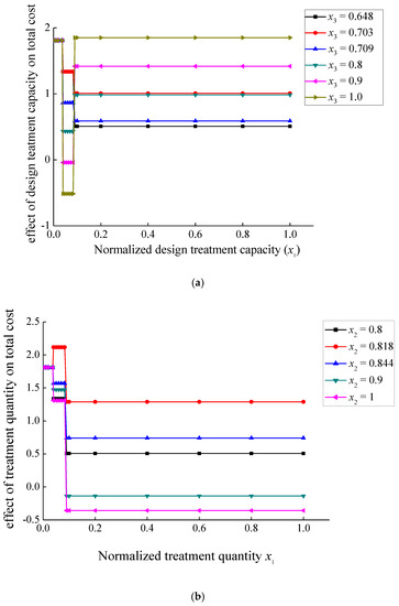
Figure 3.
(a) Effect of design treatment capacity x1 on total cost under different x3 without consideration of x2 < 0.8. (b) Effect of design treatment capacity x1 on total cost under different x2 without consideration of x3 (x3 < 0.648).
- (1)
- When x1 was less than 0.037 (DTC less than 5 m3/d), then y (TC) increased by 1.809 for each 1% increase in x1, and variables x2 (RCOD) and x3 (RNH3-N) had no effects on slope of y, which can also be seen in Figure 3a,b.
- (2)
- When x1 was less than 0.083 and greater than 0.037 (DTC was less than 10 m3/d and greater than 5 m3/d), then y (TC) depended on x1 (DTC), x2 (RCOD), and x3 (RNH3-N) together, which is described in detail as follows:
- (i)
- When x2 was less than 0.8 (RCOD less than 76.6%), then y (TC) depended on both x1 and x3 together without consideration of x2 (shown in Figure 3a). The slope of y was a constant of 1.336 when x3 was less than 0.703. When x3 ranged from 0.703 to 0.709 (i.e., RNH3-N from 65.6% to 66.1%), the slope of y decreased from 1.336 to 0.863 accordingly. When x3 ranged from 0.709 to 1.0 (RNH3-N from 66.1% to 91.89%), the slope of y decreased from 0.863 to −0.514 accordingly.
- (ii)
- When x3 was less than 0.703 (RNH3-N less than 65.6%), then y (TC) depended on both x1 and x2 together without consideration of x3 (shown in Figure 3b). When x2 ranged from 0.8 to 0.818 (RCOD from 76.6% to 78.1%), the slope of y increased from 1.336 to 2.117 accordingly. When x2 ranged from 0.818 to 0.844 (RCOD from 78.1% to 80.3%), the slope of y decreased from 2.117 to 1.568 accordingly. When x2 ranged from 0.844 to 1.0 (RCOD from 80.3% to 93.47%), the slope of y decreased from 1.568 to 1.308 accordingly.
- (iii)
- When x2 was greater than 0.8 and x3 was greater than 0.703, then the effect x1 on y was connected with the effect of both x2 and x3.
- (3)
- When x1 is greater than 0.083 (DTC greater than 10 m3/d), then y (TC) depended on x1, x2, and x3 together, which is described as follows:
- (i)
- When x2 was less than 0.8, then y (TC) depended on both x1 and x3 together without consideration of x2 (shown in Figure 3a. When x3 was less than 0.648 (RNH3-N less than 60.7%), the slope of y was a constant of 0.508. When x3 ranged from 0.648 to 0.703 (RNH3-N from 60.7% to 65.6%), the slope of y increased from 0.508 to 1.007 accordingly. When x3 ranged from 0.703 to 0.709 (RNH3-N from 65.6% to 66.1%), the slope of y decreased from 1.007 to 0.588 accordingly. When x3 ranged from 0.709 to 1.0 (RNH3-N from 66.1% to 91.89%), the slope of y increased from 0.588 to 1.851 accordingly.
- (ii)
- When x3 was less than 0.648 (RNH3-N less than 60.7%), then y (TC) depended on x1 and x2 together without consideration of x3 (shown in Figure 3b). When x2 ranged from 0.8 to 0.818 (RCOD from 76.6% to 78.1%), the slope of y increased from 0.508 to 1.288 accordingly. When x2 ranged from 0.818 to 0.844 (RCOD from 78.1% to 80.3%), the slope of y decreased from 1.288 to 0.74 accordingly. When x2 ranged from 0.844 to 1.0 (RCOD from 80.3% to 93.47%), the slope of y decreased from 0.74 to 0.48 accordingly.
- (iii)
- When x2 was greater than 0.8 and x3 was greater than 0.648, then the effect of x1 on y was connected with the effect of both x2 and x3.
Therefore, the conclusions for TC can be drawn as follows:
- (1)
- When x1 was less than 0.037 (DTC less than 5 m3/d), the slope of y (TC) was a constant of 1.809, and had no relation with neither x2 (RCOD) nor x3 (RNH3-N), which was similar to the slope of y1 (CC).
- (2)
- When x1 was greater than 0.037 and less than 0.083 (DTC range from 5 m3/d to10 m3/d), the slope of y (TC) had a relationship with both x2 (RCOD) and x3 (RNH3-N). When x2 was less than 0.8 (RCOD less than 76.6%), the slope of y had a relationship with x3 without consideration of x2. When x3 was less than 0.703 (RNH3-N less than 65.6%), the slope of y had a relationship with x2 without consideration of x3. In addition, when x2 was less than 0.8 (RCOD less than 76.6%) and x3 was less than 0.703 (RNH3-N less than 65.6%), the slope of y had no relationship with either x2 or x3.
- (3)
- When x1 was greater than 0.083 (DTC greater than 10 m3/d), the slope of y had a relationship with both x2 (RCOD) and x3 (RNH3-N). When x2 was less than 0.8 (RCOD less than 76.6%), the slope of y had a relationship with x3 without consideration of x2. When x3 was less than 0.648 (RNH3-N less than 60.7%), the slope of y had a relationship with x2 without consideration of x3. In addition, when x2 was less than 0.8 and x3 was less than 0.648 (RCOD less than 76.6% and RNH3-N less than 60.7%), the slope of y had no relationship with either x2 or x3.
The relative importance of variables and the relationship among variables are shown in Table 6, from which we can find that DTC was the most important variable in determining the total cost of sewage treatment facilities, which was the same as the results of ANOVA decomposition.
Table 6.
Relative importance of variables and their relationship.
From Table 6, we can also find that y (TC) had a significant relationship with x1 (DTC), which means that TC increased with the development of DTC. Compared with x1 (DTC), the relationship between y (TC) and x2 (RCOD), as well as the relationship between y (TC) and x3 (RNH3-N), were lower. In addition, x2 (RCOD) was more significant than x3 (RNH3-N).
The relationships among variables in the MARS model is shown in Figure 4a,b. The value of y (TC) rose with variables x1 and x2, and the contribution of x1 was greater than x2. A similar conclusion that the contribution of x1 on TC (y) was greater than x3 can be seen from Figure 4b. The results are consistent with the above analysis.
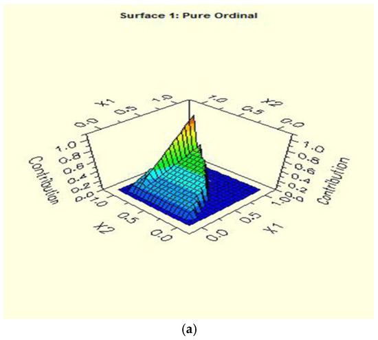
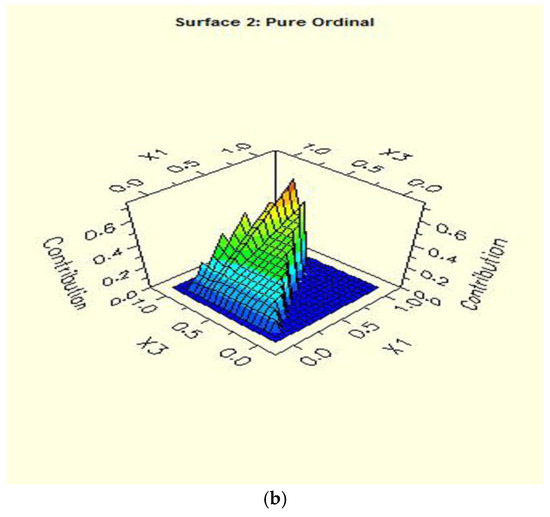
Figure 4.
(a) Contribution to total cost y of the second order term of the variables design treatment capacity (x1) and removal efficiency of chemical oxygen demand (x2). (b) Contribution to total cost y of the second order term of the variables design treatment capacity (x1) and removal efficiency of ammonia nitrogen (x3).
The total cost of building wastewater treatment plants in rural regions is an important issue concerning regional sustainable development, which is very difficult to be accurately simulated due to its nonlinear characteristics. Consequently, the multivariate adaptive regression spline (MARS) model is applied to predict the total cost of DWWTPs in this paper. The MARS model has its own advantages: (1) it does not require assumption of relationships between input and output variables, (2) automatically finds the best knots in basis functions, (3) can provide a more precise relationship between the response variable and predictor, and (4) does not require a long training process to reduce modeling time [29,30]. Therefore, the stepwise model obtained through MARS technology is a suitable method to predict total cost.
The model obtained through the MARS method was able to predict CC, OMC, and TC in DWWTPs. The comparisons of training dataset and testing dataset between real values and predicted values for CC, OMC, and TC are shown in Figure 5. In Figure 5, all the variables are in their original scale, not in the normalized scale.
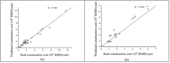
Figure 5.
(a) Comparison of training dataset between real construction cost and predicted construction cost. (b) Comparison of testing dataset between real construction cost and predicted construction cost. (c) Comparison of training dataset between real OMC and predicted OMC. (d) Comparison of testing dataset between real OMC and predicted OMC. (e) Comparison of training dataset between real total cost and predicted total cost. (f) Comparison of testing dataset between real total cost and predicted total cost.
The comparisons of the training dataset and testing dataset between real and predicted values for CC are shown in Figure 5a,b, respectively. The results of CC obtained in the training dataset were better than the results obtained in the testing dataset, which can also be observed in Table 7. The value of R for the training dataset (0.985) was greater than the value of R for the testing dataset (0.983). The comparisons of the training dataset and testing dataset between real and predicted values for OMC are shown in Figure 5c,d, respectively. The results of OMC obtained in the testing dataset were better than the results obtained in the training dataset, which can also be observed in Table 7. The value of R for the testing dataset (0.846) is greater than the value of R for the training dataset (0.753). In addition, through the MARS method, the OMC model was obtained and expressed by Equation (11). When x1 was less than 0.174 (DTC less than 20 m3/d), OMC was a constant of 435 RMB/year. Since there were 148 samples among 160 samples in the training set with DTC less than 20 m3/d, and there were 45 samples among 55 samples in the testing set with DTC less than 20 m3/d, many data points in Figure 5c,d were flat. The comparisons of training and testing datasets between real and predicted total cost (TC) are shown in Figure 5e,f, respectively. Similar to CC, the results of TC obtained in the training dataset were better than the results obtained in the testing dataset, which can also be observed in Table 7. The value of R for the training testing dataset (0.968) was greater than the value of R for the testing dataset (0.964).
Table 7.
Accuracy comparison among multivariate adaptive regression spline (MARS), support vector machine (SVM), and multiple linear regression (MLR) for the training and testing datasets.
According the results of TC, shown in Figure 5e,f, the cost of treating 1 m3 of sewage ranged from 147 RMB/year to 1512 RMB/year, with an average of 687 RMB/year.
3.3. Comparison with the Other Models
In this paper, the support vector machine (SVM) method and a multiple linear regression (MLR) model were applied to compare the results with a training set and a testing set (the same sets that were applied for validation of MARS model).
Besides the correlation coefficient of R, the accuracy performance of models were also assessed by root mean square errors (RMSE) and mean absolute percent error (MAPE), expressed by Equations (13) and (14), respectively, as follows:
The comparisons of R, RMSE, and MAPE among the three methods of MARS model, SVM model, and MLR model were calculated using Equations (9), (13), and (14), respectively, and shown in Table 7.
As can be seen, R training data values of y1 for MARS, SVM, and MLR were 0.985, 0.964, and 0.935, respectively; and R testing data values of y1 for MARS, SVM, and MLR were 0.983, 0.965, and 0.918, respectively. Results show that MARS was the fittest model of y1 in terms of maximizing R values, with a value roughly 2% above SVM, and 5% above MLR. In terms of RMSE and MAPE, the MARS model was the lowest for both training and testing data. As for y2, R training data values for MARS, SVM, and MLR were 0.753, 0.763, and 0.565, respectively; and R testing data values for MARS, SVM, and MLR were 0.846, 0.825, and 0.673, respectively. Results also indicated that the MARS model fitted y2 better than MLR and almost the same as SVM (1% below SVM for training data). In addition, R training data values of y for MARS, SVM, and MLR were 0.968, 0.964, and 0.929, respectively; and R testing data values of y for MARS, SVM, and MLR were 0.964, 0.956, and 0.904, respectively. Results also indicated that MARS was the best model to fit y.
MARS model had better statistical results with higher R values than SVM model and the MLR method. It can also be found that the simulation results of y2 for the three models were not as good as that for y1 and y as seen by the relatively lower R values. In addition, although the R values of the SVM model were closer to that of the MARS model, the RMSE and MAPE values of the SVM model were greater than that of MARS model, especially for y1 and y, which verified that the performance of the MARS model was better than the SVM model. The simulation accuracies of y, y1, and y2 for the training and testing datasets among the three models were in the order of MARS > SVM > MLR, except for y2 for the training dataset, which indicated that MARS model was a more effective method to simulate the cost structure of DWWTPs than the SVM and MLR models. Moreover, the cost structure of DWWTPs had the characteristics of being stepwise and nonlinear.
4. Conclusions
In this paper, a MARS model is proposed for predicting the cost structure of DWWTPs. The model considers the effect of DTC, RCOD, and RNH3-N on CC, OMC, and TC. The results obtained can be summarized as follows:
- (1)
- The DTC was the most important parameter for predicting CC, OMC, and TC with a relative importance of 100, followed by RCOD and RNH3-N with the relative parameters of 16.55 and 9.75, respectively.
- (2)
- The slopes of CC and TC on DTC were related to DTC, RCOD and RNH3-N, which is described in detail as follows:
- (a)
- When DTC was less than 5 m3/d, the slopes of CC and TC on DTC were constants of 1.923 and 1.809 without consideration of RCOD and RNH3-N. The constant slope means that that the relationship between CC or TC and DTC was linear. The positive and negative slopes indicated the increasing and decreasing trend, respectively. The result indicated that when DTC was less than 5 m3/d, each of the various treatment technologies with differing RCOD and RNH3-N can be chosen by planners from an economic point of view.
- (b)
- When DTC was greater than 5 m3/d, RCOD and RNH3-N affected the slopes of CC and TC of DWWTPs, which can help choose treatment technology:
- (i)
- The slopes of CC and TC on DTC had no relationship with RCOD when RCOD was less than 69.5% and 76.6%, respectively.
- (ii)
- When DTC was less than 10 m3/d, the slope of CC on DTC had no relationship with RNH3-N.
- (iii)
- When DTC was less than 10 m3/d and RNH3-N less than 60.7%, the slope of TC on DTC had no relationship with RNH3-N.
- (c)
- When DTC was greater than 10 m3/d and RNH3-N less than 65.6%, the slope of TC on DTC had no relationship with RNH3-N.
- (d)
- With the increase of DTC, the slope of CC on DTC decreased gradually from 1.923 to 1.374.
- (3)
- The slopes of OMC on DTC were related to DTC and RNH3-N described as follows:
- (a)
- When DTC was less than 20 m3/d, then OMC was a constant of 435 RMB/year, which means that 20 m3/d was the threshold for constructing DWWTPs. It can be concluded that when the treatment scale is no more than 20 m3/d, the OMC is the same at 435 RMB/year. The conclusion is meaningful and can help managers make budget between DTC and OMC.
- (b)
- When DTC was greater than 20 m3/d, then slope of OMC on DTC increased with RNH3-N and had no relationship with RCOD.
The results obtained provide useful information to perform techno-economic analysis for planners to make decisions on treatment scale and treatment technology before construction. The developed MARS model combined the merits of a nonparametric model and traditional multiple linear regression with simplicity and good interpretation, which does not need to assume a statistical distribution of the data. The non-linear structure of the cost function captured the inherent relationship between variables, which can be expected to improve the accuracy of model. Compared with SVM and MLR models, the simulation results obtained by the MARS model were closer to the real costs. The results showed that the developed MARS model can be a valuable tool to predict CC, OMC, and TC of DWWTPs. The cost–benefit evaluation can be performed more scientifically by simulating the cost structure with the proposed MARS model. The proposed method can also be applied to other regions in China to determine CC, OMC, and TC of DWWTPs based on DTC, RCOD, and RNH3-N, which can provide helpful and meaningful information for local governments to make reasonable and economic plans to protect the water environment, especially in rural regions.
Author Contributions
Writing-Review & Editing, Y.W.; Investigation, L.W.; Formal analysis, B.E.
Funding
The research was funded by the Special S&T Project on Treatment and Control of Water Pollution from Bureau of Housing and Urban-Rural Development of Changshu City (number as 2011ZX07301-003-05-04).
Acknowledgments
The data used were provided by Construction Bureau in Changshu City, and Suzhou Hongyu Wastewater Treatment Engineering Limited Corporation.
Conflicts of Interest
The authors declare no conflict of interest.
References
- Hernandez-Sancho, F.; Molinos-Senante, M.; Sala-Garrido, R. Cost modelling for wastewater treatment processes. Desalination 2011, 268, 1–5. [Google Scholar] [CrossRef]
- Zhou, Y.; Huang, G.; Zhu, H.; Li, Z.; Chen, J. A factorial dual-objective rural environmental management model. J. Clean. Prod. 2016, 124, 204–221. [Google Scholar] [CrossRef]
- Mkwate, R.C.; Chidya, R.C.G.; Wanda, E.M.M. Assessment of drinking water quality and rural household water treatment in Balaka District, Malawi. Phys. Chem. Earth 2017, 100, 353–362. [Google Scholar] [CrossRef]
- Chen, H.; Chang, N. A comparative analysis of methods to represent uncertainty in estamating the cost of constructing wastewater treatment plants. J. Environ. Manag. 2002, 65, 383–409. [Google Scholar] [CrossRef]
- Engin, G.O.; Demir, I. Cost analysis of alternative methods for wastewater handling in small communities. J. Environ. Manag. 2006, 79, 357–363. [Google Scholar] [CrossRef] [PubMed]
- Xin, X.; Huang, G.; Sun, W.; Zhou, Y.; Fan, Y. Factorial two-stage irrigation system optimization model. J. Irrig. Drain. Eng. 2016, 142, 04015056. [Google Scholar] [CrossRef]
- Papadopoulos, B.; Tsagarakis, K.P.; Yannopoulos, A. Cost and land functions for wastewater treatment projects: Typical simple linear regression versus fuzzy linear regression. J. Environ. Eng. 2007, 133, 581–586. [Google Scholar] [CrossRef]
- Friedler, E.; Pisanty, E. Effects of design flow and treatment level on construction and operation costs of municipal wastewater treatment plants and their implications on policy making. Water Res. 2006, 40, 3751–3758. [Google Scholar] [CrossRef] [PubMed]
- Lamas, W.Q.; Silveira, J.L.; Giacaglia, G.E.O.; Reis, L.O.M. Development of a methodology for cost determination of wastewater treatment based on functional diagram. Appl. Therm. Eng. 2009, 29, 2061–2071. [Google Scholar] [CrossRef]
- Khan, U.T.; Valeo, C. Comparing a Bayesian and fuzzy number approach to uncertainty quantification in short-term dissolved oxygen prediction. J. Environ. Inform. 2017, 30, 1–16. [Google Scholar] [CrossRef]
- Molinos-Senante, M.; Hernández-Sancho, F.; Sala-Garrido, R. Cost-benefit analysis of water-reuse projects for environmental purposes: A case study for Spanish wastewater treatment plants. J. Environ. Manag. 2011, 92, 3091–3097. [Google Scholar] [CrossRef]
- Chen, R.; Wang, X.C. Cost-benefit evaluation of a decentralized water system for wastewater reuse and environmental protection. Water Sci. Technol. 2009, 59, 1515–1522. [Google Scholar] [CrossRef] [PubMed]
- Wang, Y.; Wu, L.; Feng, Y. Cost function for treating wastewater in rural regions. Desalin. Water Treat. 2015, 57, 17241–17246. [Google Scholar]
- Naik, K.S.; Stenstrom, M.K. A feasibility analysis methodology for decentralized wastewater systems-energy-efficiency and cost. Water Environ. Res. 2016, 88, 201–209. [Google Scholar] [CrossRef] [PubMed]
- Maurer, M.; Rothenberger, D.; Larsen, T.A. Decentralised wastewater treatment technologies from a national perspective: At what cost are they competitive? Water Sci. Technol. Water Supply 2006, 5, 145–154. [Google Scholar] [CrossRef]
- Zhang, W.; Zhang, Y.; Goh, A.T.C. Multivariate adaptive regression splines for inverse analysis of soil and wall properties in braced excavation. Tunn. Undergr. Space Technol. 2017, 64, 24–33. [Google Scholar] [CrossRef]
- Zarei, K.; Atabati, M.; Teymori, E. Multivariate adaptive regression splines for prediction of rate constants for radical degradation of aromatic pollutants in water. J. Solut. Chem. 2014, 43, 445–452. [Google Scholar] [CrossRef]
- Samui, P.; Kim, D. Determination of the angle of shearing resistance of soils using multivariate adaptive regression spline. Mar. Georesour. Geotechnol. 2014, 33, 542–545. [Google Scholar] [CrossRef]
- Nieto, P.J.G.; Fernández, J.R.A.; Lasheras, F.S.; Juez, F.J.D.; Muñiz, C.D. A new improved study of cyanotoxins presence from experimental cyanobacteria concentrations in the Trasona reservoir (Northern Spain) using the MARS technique. Sci. Total Environ. 2012, 430, 88–92. [Google Scholar] [CrossRef]
- Menon, R.; Bhat, G.; Saade, G.R.; Spratt, H. Multivariate adaptive regression splines analysis to predict biomarkers of spontaneous preterm birth. Acta Obstet. Gynecol. Scand. 2014, 93, 382–391. [Google Scholar] [CrossRef] [PubMed]
- Lee, T.S.; Chen, I.F. A two-stage hybrid credit scoring model using artificial neural networks and multivariate adaptive regression splines. Expert Syst. Appl. 2005, 28, 743–752. [Google Scholar] [CrossRef]
- Molinos-Senante, M.; Garrido-Baserba, M.; Reif, R.; Hernández-Sancho, F.; Poch, M. Assessment of wastewater treatment plant design for small communities: Environmental and economic aspects. Sci. Total Environ. 2012, 427–428, 11–18. [Google Scholar] [CrossRef] [PubMed]
- Chen, Y.; Fan, R.; Liu, Z.; Chen, P. Research progress of integrated rural domestic sewage treatment plant. J. Anhui Agric. Sci. 2016, 44, 84–88. (In Chinese) [Google Scholar]
- Chang, L. Analysis of bilateral air passenger flows: A non-parametric multivariate adaptive regression spline approach. J. Air Transp. Manag. 2014, 34, 123–130. [Google Scholar] [CrossRef]
- Friedman, J.H. Multivariate adaptive regression splines. Ann. Stat. 1991, 19, 1–67. [Google Scholar] [CrossRef]
- Haghiabi, A.H. Prediction of river pipeline scour depth using multivariate adaptive regression splines. J. Pipeline Syst. Eng. 2017, 8, 04016015. [Google Scholar] [CrossRef]
- Samui, P. Multivariate adaptive regression spline (Mars) for prediction of elastic modulus of jointed rock mass. Geotech. Geol. Eng. 2013, 31, 249–253. [Google Scholar] [CrossRef]
- Cheng, M.; Cao, M. Estimating strength of rubberized concrete using evolutionary multivariate adaptive regression splines. J. Civ. Eng. Manag. 2016, 22, 711–720. [Google Scholar] [CrossRef]
- Chang, L. Exploring contributory factors to highway accidents: A nonparametric multivariate adaptive regression spline approach. J. Transp. Saf. Secur. 2017, 9, 419–438. [Google Scholar] [CrossRef]
- Fernández, J.R.A.; Nieto, P.J.G.; Muniz, C.D.; Antón, J.C.Á. Modeling eutrophication and risk prevention in a reservoir in the Northwest of Spain by using multivariate adaptive regression splines analysis. Ecol. Eng. 2014, 68, 80–89. [Google Scholar] [CrossRef]
© 2019 by the authors. Licensee MDPI, Basel, Switzerland. This article is an open access article distributed under the terms and conditions of the Creative Commons Attribution (CC BY) license (http://creativecommons.org/licenses/by/4.0/).