Modelling of Erosion and Transport Processes

Abstract

Erosion phenomena are the result of complicated natural processes. The determination of their course, their mathematical expression, and predicting erosion phenomena of certain intensities is an important hydrological problem. To obtain a solution, it is necessary to evaluate the erosion factors in detail, which act by the origin and course of erosion processes, to analyse their influences, and to apply correct conclusions to their complex activity on this basis. Dimensional analysis is a conceptual tool often applied in engineering to understand physical situations involving a mix of different kinds of physical quantities. It is routinely used by physical scientists and engineers to check the plausibility of derived equations and computations. It is also used to form reasonable hypotheses about complex physical situations that can be tested by experiment or by more developed theories of the phenomena. In this paper, the dimensional analysis is used for the modelling of erosion and transport processes.

1. Introduction

Water erosion is a widespread phenomenon in Eastern Europe. Surface runoff destroys and removes the topsoil layer and deposits it at the foot of slopes or transports it to streams. Significant losses in the national economy occur; they consist especially in the decrease of valuable topsoil and in the loss of the plants’ nutrients by which agriculture is weakened in its production bases. Soil particles washed into streams are the main source of sediments, which threaten their profiles, reservoirs, ponds, and weirs by silting; thus arises the question of the existence and rentability of hydraulic structures and, simultaneously, other important questions, such as unnecessary inundations and increasing the underground water level in the closed area.

Soil loss from intensively agriculturally cultivated lands causes water pollution, which is unfavourable especially for water supply reservoirs, which become important elements in conveying potable water for the inhabitants in the country. Stream erosion causes unfavourable sediment regimes with all its consequences. The most important factors causing the origin and influencing the course of water erosion in watersheds are climatic and hydrologic factors, morphological factors–slope gradient, slope length, shape of the slope, exposure of the slope, soil factors, geological factors, vegetation factors, cropping management, and socio-economic factors [1].

These factors may be used for erosion and transport processes modelling. In engineering, the application of designs makes use of empirical results from a lot of experiments. This data is often difficult to present in a readable form. Dimensional analysis provides a strategy for choosing relevant data and how it can be presented. This is a useful technique in all experimentally-based areas of engineering. If it is possible to identify the factors involved in a physical situation, dimensional analysis can form a relationship between them.

According to [2], the most widely used approaches during an 80-year history of erosion modelling are Universal Soil Loss Equation (USLE)-type based algorithms, which have been applied in 109 countries. Model comparisons demonstrate that the application of process-based physical models (e.g., WEPP or PESERA) does not necessarily result in lower uncertainties compared to more simple structured empirical models, such as USLE-type algorithms.

Empirical erosion models such as the Revised Universal Soil Loss Equation (RUSLE) provides a rather simple and yet comprehensive framework for assessing soil erosion and its causative factors [3]. Soil erosion is a serious problem arising from agricultural intensification, land degradation, and other anthropogenic activities. In the study [4], the soil loss model, Revised Universal Soil Loss Equation (RUSLE) integrated with GIS, has been used to estimate soil loss in the Nethravathi Basin located in the southwestern part of India. The Nethravathi Basin is a tropical coastal humid area with a drainage area of 3128 km² up to the gauging station. The parameters of the RUSLE model were estimated using remote sensing data, and the erosion probability zones were determined using GIS. The estimated rainfall erosivity, soil erodibility, topographic, and crop management factors range from 2948.16 to 4711.4 MJ·mm·ha⁻¹h⁻¹year⁻¹, 0.10 to 0.44 t·h·MJ⁻¹·mm⁻¹, 0 to 92.774, and 0 to 0.63, respectively.

In [5], a comprehensive methodology that integrates the Revised Universal Soil Loss Equation (RUSLE) model and Geographic Information System (GIS) techniques, was adopted to determine the soil erosion vulnerability of a forested mountainous sub-watershed in Kerala, India. The resultant map of annual soil erosion shows a maximum soil loss of 17.73 t ha⁻¹ year⁻¹ with a close relation to grassland areas, degraded forests, and deciduous forests on the steep side-slopes (with high LS) [5].

Very susceptible to soil erosion, due to its complicated terrain and heavy rainfall, is Central Vietnam. In [6], soil erosion was quantified in the Sap river basin, Vietnam, using the Universal Soil Loss Equation (USLE) and Geographical Information System (GIS). The results showed that soil erosion was most sensitive to the topographic factor (LS), followed by the practice support factor (P), soil erodibility factor (K), cropping management (C), and the rainfall erosivity factor (R). Implications are that changes to the cultivated calendar and implementing intercropping are effective ways to prevent soil erosion in cultivated lands [6].

The estimate of the soil erodibility factor (K-factor) using a Universal Soil Loss Equation (USLE) nomograph, and an evaluation of the spatial distribution of the predicted K-factor in a mountainous agricultural watershed in the northwestern Amhara region, Ethiopia, was a subject in [7].

Soil erosion is a problem of global significance for land management [8]. Attempts to assess soil erosion by water encompass plot studies, monitoring, modelling, and the use of tracers. All of these approaches are shown to have shortcomings, calling into question the reliability of current estimates. There is an urgent need to develop approaches to estimating rates of soil erosion that are consistent with the current understanding of erosion processes [8]. Only then, reliable estimates of soil erosion can be made on which reliable land-use and policy decisions should be based.

2. Materials and Methods

It is necessary to know the loss of soil in the watersheds in order to state the rate of water erosion. For determination of soil loss, numerous methods are used. The well-known method is the Universal Soil Loss Equation or its revised version.

The Universal Soil Loss Equation (USLE) predicts the long-term average annual rate of erosion on a field slope based on rainfall pattern, soil type, topography, crop system, and management practices. USLE only predicts the amount of soil loss that results from sheet and rill erosion on a single slope and does not account for additional soil losses that might occur from gully, wind, or tillage erosion. This erosion model was created for use in selected cropping and management systems but is also applicable to non-agricultural conditions, such as construction sites. The USLE can be used to compare soil losses from a particular field with a specific crop and management system to “tolerable soil loss” rates. Alternative management and crop systems may also be evaluated to determine the adequacy of conservation measures in farm planning.

Five major factors are used to calculate the soil loss for a given runoff profile. Each factor is the numerical estimate of a specific condition that affects the severity of soil erosion at a particular location. The erosion values reflected by these factors can vary considerably due to varying weather, soil, morphological, and tillage conditions. Therefore, the values obtained from the USLE more accurately represent long-term averages. Universal Soil Loss Equation (USLE) has the form [9]:

$$O \left(soil loss\right) = R \times K \times LS \times C \times P$$

(1)

where O represents the potential long-term average annual soil loss in tons per acre (hectare) per year. This is the amount that is compared to the “tolerable soil loss” limits.

R is the rainfall and runoff factor by geographic location. The greater the intensity and duration of the rain storm, the higher the erosion potential.

K is the soil erodibility factor. It is the average soil loss in tons/acre per R-unit for a particular soil in cultivated, continuous fallow, with an arbitrarily selected slope length of 72.6 feet and slope steepness of 9%.

LS is the slope length-gradient factor. The LS factor represents a ratio of soil loss under given conditions to that at a site with the “standard” slope steepness of 9% and slope length of 72.6 feet. The steeper and longer the slope, the higher the risk of erosion.

C is the crop/vegetation and management factor. The C factor can be determined by selecting the crop type and tillage method that corresponds to the field and then multiplying these factors together.

P is the support practice factor. It reflects the effects of practices that will reduce the amount and rate of the water runoff and, thus, reduce the amount of erosion. The most commonly used supporting cropland practices are cross slope cultivation and contour farming.

With additional research, experiments, data, and resources becoming available, research scientists continued to improve USLE, which led to the development of the Revised Universal Soil Loss Equation (RUSLE). RUSLE has the same formula as USLE but has several improvements in determining factors. These include some new and revised isoerodent maps, a time-varying approach for soil erodibility factor, a sub-factor approach for evaluating the cover-management factor, a new equation to reflect slope length and steepness, and new conservation-practice values [10].

3. Results

For soil loss assessment, the watershed Kamenice was chosen. Kamenice is situated in southern Bohemia. The main water course in the river watershed is the Kamenice River, which catches water from the watershed into the watershed Květoňov. The area of the river watershed is 32.15 km². It is spread in broken relief. The soil in the watershed is used mainly for agriculture [11]. The situation of the watershed Květoňov is shown in Figure 1. The obtained values of the relevant parameters are introduced in

Table 1. Values of relevant arguments.

Plot	S (m2)	L (m)	i (m/s)	ρ (kg/m3)	K (m/s)	C (−)	Sf (−)
1	25,000	110	2.63 × 10−8	1880	4.0 × 10−6	0.005	1.7536
2	15,000	100	2.63 × 10−8	1880	4.0 × 10−6	0.005	1.3508
3	255,000	970	2.63 × 10−8	1850	7.0 × 10−6	0.610	1.0016
4	72,000	290	2.63 × 10−8	1850	7.0 × 10−6	0.610	1.4117
5	71,000	260	2.63 × 10−8	1850	7.0 × 10−6	0.005	1.1689
6	132,000	700	2.63 × 10−8	1850	1.5 × 10−5	0.610	0.7357
7	48,000	290	2.63 × 10−8	1850	7.0 × 10−6	0.610	1.0000
8	289,000	1460	2.63 × 10−8	1840	2.5 × 10−6	0.610	1.2113
9	29,000	180	2.63 × 10−8	1850	7.0 × 10−6	0.005	0.5712
10	53,000	560	2.63 × 10−8	1850	7.0 × 10−6	0.092	0.4778
11	65,000	350	2.63 × 10−8	1850	7.0 × 10−6	0.005	3.1411
12	59,000	240	2.63 × 10−8	1850	7.0 × 10−6	0.005	2.0019
13	39,000	160	2.63 × 10−8	1850	7.0 × 10−6	0.005	3.2743
14	50,000	500	2.63 × 10−8	1850	1.5 × 10−5	0.005	0.4544
15	46,000	160	2.63 × 10−8	1850	1.5 × 10−5	0.005	1.7730
16	118,000	950	2.63 × 10−8	1870	1.5 × 10−5	0.005	1.2783
17	54,000	370	2,63 × 10−8	1850	1.0 × 10−5	0.005	1.5781
18	34,000	130	2,63 × 10−8	1900	2.5 × 10−6	0.005	1.7536
19	37,000	120	2.63 × 10−8	1850	7.0 × 10−6	0.092	1.9745
20	245,000	620	2.63 × 10−8	1850	1.5 × 10−5	0.092	1.3735
21	60,000	450	2.63 × 10−8	1900	2.5 × 10−6	0.005	1.1689
22	34,000	130	2.63 × 10−8	1850	1.5 × 10−5	0.050	0.8440
23	126,000	650	2.63 × 10−8	1900	2.5 × 10−6	0.005	1.0294
24	412,000	2400	2.63 × 10−8	1850	7.0 × 10−6	0.092	1.2710
25	34,000	130	2.63 × 10−8	1850	7.0 × 10−6	0.005	1.5457
26	171,000	750	2.63 × 10−8	1850	7.0 × 10−6	0.005	1.8802
27	99,000	460	2.63 × 10−8	1850	7.0 × 10−6	0.005	1.1066
28	231,000	1520	2.63 × 10−8	1800	1.0 × 10−5	0.005	0.8188

. The plots (1–28) near river banks, grassed or agriculturally used, are considered.

For the determination of soil loss in watersheds by using dimensional analysis, it is essential to state parameters that characterise water erosion in river watersheds, and it is possible to measure them. From the known state of the art, the following variables are selected [12]:

• Rainfall intensity	i	(m·s−1)
• Soil density	ρ	(kg·m−3)
• Area of the plot	S	(m2)
• Length of the plot	L	(m)
• Filtration coefficient	K	(m·s−1)
• Vegetation factor (from USLE)	C	(-)
• Coefficient of the slope steepness	Sf	(-)
• Soil loss (from plot)	O	[kg/(m2·s)] or (kg·m−2·s−1)

All the given variables are presented in basic dimensions, which is the condition for dimensional analysis application. All these variables are measurable, or it is possible to state them. It is a rather complex issue to measure soil loss exactly. Results of soil losses obtained from RUSLE [13] are used for the development of the model based on dimensional analysis.

Developed models describing water erosion in watersheds are based on the formation of dimensionless arguments π_i from the stated variables influencing erosion. Their valuable property is that in all existing systems of units, they have the same numerical size and they have no dimension. Formation of the model consists of the derivation of functional dependence from the expressed dimensionless variables, which in general, always has an exponential character. Transformation of this function into logarithmic coordinates corresponds to linear characters that make work with the model easier and enables the determination of the parameters of linear function [12].

The general relation among the selected variables, which can affect the erosion in a watershed, can be expressed in the form:

$$\phi \left(i,\rho , S, L, K, C, S_f, O\right) = 0.$$

(2)

The following equation is valid:

$${\pi }_i = i^{x_1} \times L^{x_2} \times S^{x_3} \times {\rho }^{x_4} \times O^{x_5} \times K^{x_6} \times C^{x_7} \times S_f^{x_8}.$$

(3)

The dimension of velocity occurs twice among selected variables; therefore, the rate K/i is the rate of two variables with the same dimension and presents a dimensionless argument—a simplex that will be included in the solution. Dimensionless variables S_f and C present simplexes, too.

The dimensional matrix-relation (4) for basic units has the rank of matrix m = 3, and its lines are dimensionally independent on themselves. The form of the matrix is:

$$\begin{array}{cccccc} \hfill & i\hfill & L\hfill & S\hfill & \rho \hfill & O\hfill \\ \mathrm{kg}\hfill & 0\hfill & 0\hfill & 0\hfill & 1\hfill & 1\hfill \\ \mathrm{m}\hfill & 1\hfill & 1\hfill & 2\hfill & \mathrm{-3}\hfill & \mathrm{-2}\hfill \\ \mathrm{s}\hfill & \mathrm{-1}\hfill & 0\hfill & 0\hfill & 0\hfill & \mathrm{-1}\hfill \end{array}$$

(4)

From n = 5, independent variables at the rank of the matrix m can be set up as i = n – m, that is, 2 dimensionless arguments π.

Because the number of the unknown parameters x_i > m, it is impossible to determine them clearly. The matrix (4) is divided into two parts, as well as unknown variables x_i. Then, it is modified for the solution in the way that its determinant is not equal to zero. The form of the matrix (4) is the following:

$$A \times B = \left(-1\right) \times D \times E.$$

(5)

Equation (5) has the form (6) after modification:

$$\left|\begin{array}{ccc}0& 0& 1\\ 1& 1& -3\\ -1& 0& 0\end{array}\right| \times \left|\begin{array}{c}{x}_1\\ x_2\\ x_4\end{array}\right| = \left(-1\right) \times \left|\begin{array}{cc}+1& 0\\ -2& 2\\ -1& 0\end{array}\right| \times \left|\begin{array}{c}{x}_5\\ x_3\end{array}\right| .$$

(6)

The determinant is calculated according to Laplace’s equation:

$${\mathsf{\Delta }}_A = \Sigma {\left(–1\right)}^{i+j} \times a_{ij} \times M_{ij}$$

(7)

where a_ij is the element in rank i and column j, and M_ij is the sub-determinant of the matrix. The determinant of the matrix is Δ_A = 1.

The choice of the unknown parameters x₅ and x₃ is done twice, while the selections are independent. The matrix of the selections has the form:

$$\begin{array}{ccc} \hfill & x_5\hfill & x_3\hfill \\ 1.\mathrm{choice}\hfill & 1\hfill & 0\hfill \\ 2.\mathrm{choice}\hfill & 0\hfill & 1\hfill \end{array}$$

(8)

Its determinant is Δ = 1, so the condition of the solvability is completed. It reaches the following according to (4) by multiplying matrixes:

$${\left[A\right]}_{3 \times 3} \times {\left[B\right]}_{3 \times 1} = {\left[C\right]}_{3 \times 1}$$

(9)

$${\left[D\right]}_{3 \times 2} \times {\left[E\right]}_{2 \times 1} = {\left[F\right]}_{3 \times 1}.$$

(10)

According to (5), the following is valid:

$${\left[C\right]}_{3 \times 1} = \left(-1\right) \times {\left[F\right]}_{3 \times 1}$$

(11)

The type of the matrixes in relation to (11) is the same, so for the simple elements, according to the matrix (6), the system of three linear equations with five unknown parameters is valid:

$$\begin{gathered} x_4 = -x_5 \\ {x}_1+x_2-3x_4 = 2x_5-2x_3 \\ -x_1 = x_5. \end{gathered}$$

(12)

Two independent vectors (13) are obtained by the solution of the system of linear equations (12):

$$\begin{array}{cccccc} \hfill & x_1\hfill & x_2\hfill & x_3\hfill & x_4\hfill & x_5\hfill \\ {\pi }_1\hfill & \mathrm{-1}\hfill & 0\hfill & 0\hfill & \mathrm{-1}\hfill & 1\hfill \\ {\pi }_2\hfill & 0\hfill & \mathrm{-2}\hfill & 1\hfill & 0\hfill & 0\hfill \end{array}$$

(13)

Two complex dimensionless arguments correspond to this solution in the forms:

$${\pi }_1 = O^1 \times i^{-1} \times {\rho }^{-1}$$

(14)

$${\pi }_2 = S^1 \times L^{-2}.$$

(15)

The third argument is the rate of two variables with the same dimension:

$$\begin{array}{cc}{x}_6\hfill & x_1\hfill \\ 1\hfill & \mathrm{-1}.\hfill \end{array}$$

(16)

The form of the dimensionless argument is:

$${\pi }_3 = K^1 \times i^{-1}.$$

(17)

The next dimensionless arguments are:

$${\pi }_4 = S_f$$

(18)

$${\pi }_5 = C.$$

(19)

The searched dimensional homogeneous function describes the loss of soil in the dimensionless form:

$$\phi \left({\pi }_1, {\pi }_2, {\pi }_3, {\pi }_4,{\pi }_5\right) = 0.$$

(20)

After adjustment and backward transformation of dimensions for the particular variables, the function has the form:

$$\phi \left(\frac{O}{i \times \rho }, \frac{S}{L^2}, \frac{K}{i},S_f,C\right) = 0.$$

(21)

Dimensionless argument π₁ contains the unknown parameter O; therefore, this argument can be expressed like the function of the other arguments in the form:

$${\pi }_1 = \phi \left({\pi }_2, {\pi }_3, {\pi }_4,{\pi }_5\right).$$

(22)

Now, we are searching for the dependence of arguments π₁ and π₂. The relation between independent argument π₂ and dependent argument π₁ can be defined by the exponential equation:

$${\pi }_1 = A \times {\pi }_2^B.$$

(23)

The real course of the dependence (23) of the dimensionless arguments π₁ and π₂ in logarithmic coordinates is depicted in Figure 2. The relation (23) is transformed into linear dependence by logarithmic calculation:

$$\log {\pi }_1 = \log A + B \times \log {\pi }_2.$$

(24)

The straight regression line for the calculation of the regression coefficients can be calculated by the method of least squares:

$$a = \frac{{{\displaystyle \sum }}^{}{x}_i^2 \times {{\displaystyle \sum }}^{}{y}_i - {{\displaystyle \sum }}^{}{x}_i \times {{\displaystyle \sum }}^{}{x}_i \times y_i}{n \times {{\displaystyle \sum }}^{}{x}_i^2 - {({{\displaystyle \sum }}^{}{x}_i)}^2},$$

(25)

$$b = \frac{n \times {{\displaystyle \sum }}^{}{x}_i \times y_i - {{\displaystyle \sum }}^{}{x}_i \times y_i}{n \times {{\displaystyle \sum }}^{}{x}_i^2 - {({{\displaystyle \sum }}^{}{x}_i)}^2}.$$

(26)

where ${{\displaystyle \sum }}^{}{x}_i={{\displaystyle \sum }}^{}\log {\pi }_2$ and ${{\displaystyle \sum }}^{}{y}_i={{\displaystyle \sum }}^{}\log {\pi }_1$. Because a =log A:

$$A = {10}^a,$$

(27)

$$B = b.$$

(28)

After completing the relation (23), the following equation is obtained:

$$\frac{O}{i \times \rho } = A \times {\left(\frac{S}{L^2}\right)}^B.$$

(29)

After modification of the relation (29), the following equation is valid:

$$O = A \times S^{B } \times i \times \rho \times L^{-2B}.$$

(30)

Considering other dimensionless arguments, the relation characterising soil loss in river watersheds has the final form:

$$O = A \times S^B \times i \times \rho \times L^{-2B} \times X \times Y \times Z$$

(31)

where X, Y, Z are dependences of the other dimensionless arguments on variables defined in the next part. Relation (31) presents the model of soil loss in watersheds.

According to Equations (14) and (15), the dimensionless arguments π₁ and π₂ are calculated. The values of these arguments are presented in

Table 2. Values of dimensionless arguments, calculated soil loss, and uncertainty.

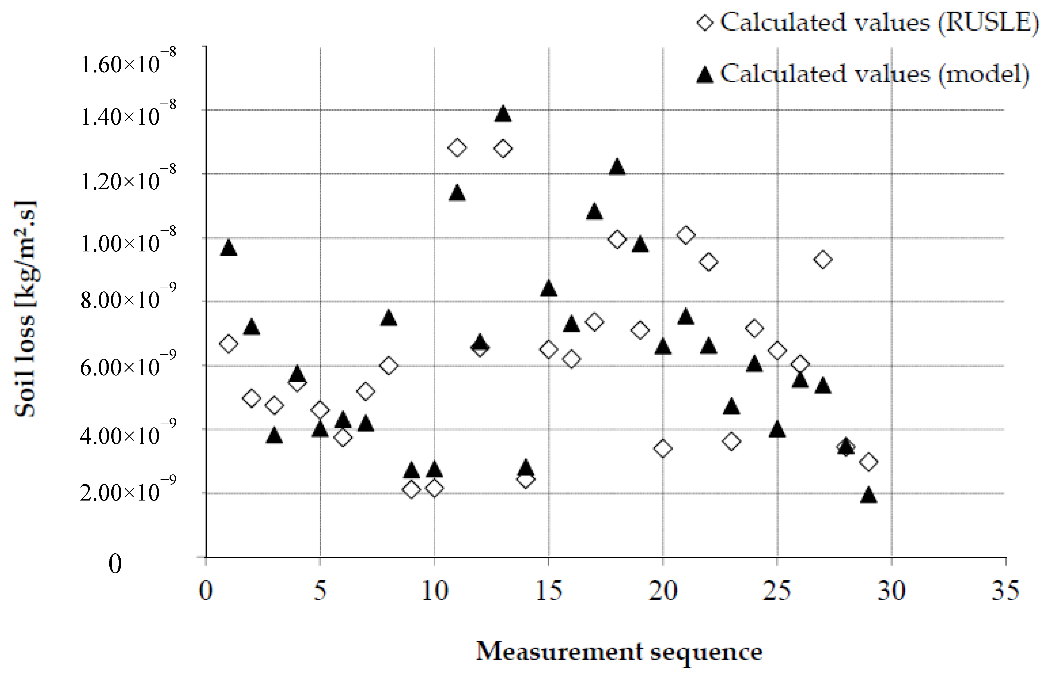
Plot	π1	π2	ORUSLE [kg/(m2·s)]	Omodel [kg/(m2·s)]	σ (%)
1	1.35 × 10−4	2.066116	6.681 × 10−9	9.707 × 10−9	45.289
2	1.01 × 10−4	1.500000	4.975 × 10−9	7.234 × 10−9	45.413
3	9.77 × 10−5	0.271017	4.756 × 10−9	3.832 × 10−9	19.430
4	1.12 × 10−4	0.856124	5.466 × 10−9	5.764 × 10−9	5.450
5	9.46 × 10−5	1.050296	4.607 × 10−9	4.030 × 10−9	12.526
6	7.70 × 10−5	0.269388	3.748 × 10−9	4.322 × 10−9	15.316
7	1.07 × 10−4	0.570749	5.190 × 10−9	4.207 × 10−9	18.943
8	1.24 × 10−4	0.135579	5.999 × 10−9	7.512 × 10−9	25.220
9	4.34 × 10−5	0.895062	2.115 × 10−9	2.735 × 10−9	29.326
10	4.44 × 10−5	0.169005	2.162 × 10−9	2.768 × 10−9	28.018
11	2.63 × 10−4	0.530612	1.282 × 10−8	1.142 × 10−8	10.940
12	1.35 × 10−4	1.024306	6.567 × 10−9	6.756 × 10−9	2.885
13	2.63 × 10−4	1.523438	1.279 × 10−8	1.391 × 10−8	8.688
14	5.01 × 10−5	0.200000	2.438 × 10−9	2.826 × 10−9	15.908
15	1.34 × 10−4	1.796875	6.506 × 10−9	8.435 × 10−9	29.639
16	1.26 × 10−4	0.130748	6.202 × 10−9	7.322 × 10−9	18.054
17	1.51 × 10−4	0.394490	7.366 × 10−9	1.084 × 10−8	47.202
18	1.99 × 10−4	2.011834	9.953 × 10−9	1.224 × 10−8	23.033
19	1.46 × 10−4	2.569444	7.109 × 10−9	9.828 × 10−9	38.248
20	2.07 × 10−4	0.637357	1.008 × 10−8	7.553 × 10−8	25.118
21	1.85 × 10−4	0.296296	9.243 × 10−9	6.634 × 10−9	28.224
22	7.44 × 10−5	2.011834	3.624 × 10−9	4.742 × 10−9	30.850
23	1.43 × 10−4	0.298225	7.166 × 10−9	6.073 × 10−9	15.250
24	1.33 × 10−4	0.071528	6.468 × 10−9	4.026 × 10−9	37.753
25	1.24 × 10−4	2.011834	6.043 × 10−9	5.566 × 10−9	7.898
26	1.91 × 10−4	0.304000	9.322 × 10−9	5.385 × 10−9	42.235
27	7.09 × 10−5	0.467864	3.450 × 10−9	3.495 × 10−9	1.304
28	6.29 × 10−5	0.099983	2.980 × 10−9	1.957 × 10−8	34.324

. Additionally, the values of soil losses are presented in Table 2. Soil losses are calculated from the developed model based on dimensionless analysis (O_model). These values are compared with soil losses calculated from the existing Universal Soil Loss Equation (O_RUSLE). The differences between the values O_RUSLE and O_model are expressed as uncertainty, which is computed from equation:

$$\sigma = \frac{1 }{n} \times {\displaystyle \sum }_{i=1}^n\frac{\left|O_{RUSLE}-O_{model}\right|}{O_{RUSLE}} \times 100.$$

(32)

The average value of the uncertainty for this case is 26.1%.

Figure 2 depicts the dependency of dimensionless arguments π₁ and π₂. The regression equation is in the form:

$$y = 0.0001 \times x^{0.1268}$$

(33)

where y is the dependent argument π₁, and x is the independent argument π₂. The regression coefficients are then A = 0.0001 and B = 0.1268.

The values of soil loss are calculated according to relation (31) on the base of relevant input parameters and calculated coefficients A and B. The final form of the developed model for stating soil loss-is:

$$O = 0.000123 \times S^{0.12684 } \times i \times \rho \times L^{-0.25368} \times X \times Y \times Z$$

(34)

where $X = 0.0011{\left(\frac{K}{i}\right)}^2 - 0.8284\left(\frac{K}{i}\right) + 226.14$,

$$\begin{gathered} Y = 0.0455C^2 - 0.0311C + 0.0072, \\ Z = 0.2312S_f^{2 }- 0.1573S_f + 0.5882. \end{gathered}$$

(35)

Equation for S_f is obtained from literature [14,15]:

$$S_f = \frac{\left(0.43 + 0.30\alpha + 0.043{\alpha }^2\right) }{6.613}$$

(36)

where α is slope (%).

The coefficients X, Y, Z present dimensionless argument-dependences π₃, π₄, π₅ or K/i, C-factor, S_f on π₁, according to relation (22). These dependences are determined from regression lines by using the software MS Excel.

4. Discussion

A comparison of the soil loss values calculated from USLE and from the developed model is shown in Figure 3. Differences between calculated and measured values occurred because of not considering the same exact influences.

The rate of erosion threat in a watershed depends on soil loss (O). The authors of [16] state the following:

• No or low erosion is if O (t/ha/year) <4;
• Medium erosion is if O (t/ha/year) 4–8;
• High erosion is if O (t/ha/year) 8–12;
• Very high erosion is if O (t/ha/year) >12.

Average soil loss (O_model) in this watershed is 9.53 t/ha/year. There is high erosion according to the mentioned dividing.

The developed model (34) represents a new approach for soil loss calculation and, following this, for water erosion determination in watersheds.

5. Conclusions

Water erosion causes serious problems in watersheds. Movement of sediment and associated agricultural pollutants into watercourses is the major impact resulting from erosion. This leads to sedimentation in watercourses and dams, disruption of the ecosystems of lakes, and contamination of drinking water. A more minor effect can occur in situations where eroded soil has a decreased capacity to absorb water: increased runoff may lead to downstream flooding and local damage to property.

In this paper, the dimensional analysis is used for soil loss modelling as the main impact of water erosion in watersheds. Dimensional analysis is a method widely used in environmental engineering as well as in water management. However, there are no references about using dimensionless analysis for the modelling of erosion and transport processes in watersheds. The average uncertainty (variation) of the developed model is 26.1%. This is an appropriate value for modelling such phenomena as soil loss in watersheds. As was already mentioned, soil loss in watersheds is influenced by numerous factors. The differences between the calculated values O_RUSLE and O_model could occur mainly because of the variables selection, and all relevant variables may not have been included. It is still possible to use the developed model for soil loss determination as well as the rate of water erosion statement. It will be valuable to use this model for verification in the conditions of Slovakia, even though there is a great requirement for input data.

References

- Zeleňáková, M.; Ondrejka Harbuľáková, V.; Karaszová, Z. Soil erosion risk in the catchment area of the water reservoirs. In Public Recreation and Landscape Protection–with Man Hand in Hand; Mendel University: Brno, Czechia, 2015; pp. 227–232. [Google Scholar]
- Alewell, C.H.; Borrelli, P.; Meusburger, K.; Panagos, P. Using the USLE: Chances, challenges and limitations of soil erosion modelling. Int. Soil Water Conserv. Res. 2019, 7, 203–225. [Google Scholar] [CrossRef]
- Phinzi, K.; Ngetar, N.S. The assessment of water-borne erosion at catchment level using GIS-based RUSLE and remote sensing: A review. Int. Soil Water Conserv. Res. 2019, 7, 27–46. [Google Scholar] [CrossRef]
- Ganasri, B.P.; Ramesh, H. Assessment of soil erosion by RUSLE model using remote sensing and GIS—A case study of Nethravathi Basin. Geosci. Front. 2016, 7, 953–961. [Google Scholar] [CrossRef]
- Prasannakumar, V.; Vijith, H.; Abinod, S.; Geetha, N. Estimation of soil erosion risk within a small mountainous sub-watershed in Kerala, India, using Revised Universal Soil Loss Equation (RUSLE) and geo-information technology. Geosci. Front. 2012, 3, 209–215. [Google Scholar] [CrossRef]
- Pham, T.G.; Degener, J.; Kappas, M. Integrated Universal Soil Loss Equation (USLE) and Geographical Information System (GIS) for soil erosion estimation in A Sap basin: Central Vietnam. Int. Soil Water Conserv. Res. 2018, 6, 99–110. [Google Scholar] [CrossRef]
- Addis, H.K.; Klik, A. Predicting the spatial distribution of soil erodibility factor using USLE nomograph in an agricultural watershed, Ethiopia. Int. Soil Water Conserv. Res. 2015, 3, 282–290. [Google Scholar] [CrossRef]
- Parsons, A.J. How reliable are our methods for estimating soil erosion by water? Sci. Total Environ. 2019, 676, 215–221. [Google Scholar] [CrossRef] [PubMed]
- Wischmeier, W.H.; Smith, D.D. Predicting Rainfall Erosion Losses. A Guide to Conservation Planning; Agriculture Handbook; U.S Department of Agriculture: Washington, DC, USA, 1978.
- Šlezingr, M.; Pilařová, P.; Pelikán, P.; Zeleňáková, M. Verification and proposal of the modification of “the method for the establishment of the erosion terminant”. Acta Univ. Agric. Silvic. Mendeleianae Brun. 2012, 60, 303–308. [Google Scholar] [CrossRef]
- Jakubíková, A. Using of RUSLE Software for Erosion Endangerment Determination in Condition of Czech Republic. Ph.D. Thesis, ČVUT, Praha, Czech Republic, 2004. (In Czech). [Google Scholar]
- Čarnogurská, M. Dimensional Analysis and Similarity Theory and Modelling in Practice; Elfa: Košice, Slovakia, 1998; p. 64. (In Slovak) [Google Scholar]
- Henriczy, G. Erosion and Transport Processes Evaluation by Using Geographical Information Systems. Bachelor’s Thesis, SvF TU, Košice, Slovakia, 2016. (In Slovak). [Google Scholar]
- Fulajtár, E.; Janský, L. Water Erosion of Soil and Erosion Protection; VÚPOP: Bratislava, Slovakia, 2001; p. 310. (In Slovak) [Google Scholar]
- Holý, M. Erosion and Environment; ČVUT: Praha, Czech Republic, 1994; p. 383. (In Czech) [Google Scholar]
- Heinige, V. Watershed Protection and Management; STU: Bratislava, Slovakia, 1995; p. 180. (In Slovak) [Google Scholar]