Article

Numerical Simulation Study on Salt Release Across the Sediment–Water Interface at Low-Permeability Area

School of Earth Sciences and Engineering, Hohai University, Nanjing 211100, China
*
Author to whom correspondence should be addressed.
Water 2019, 11(12), 2503; https://doi.org/10.3390/w11122503
Submission received: 10 October 2019 / Revised: 25 November 2019 / Accepted: 25 November 2019 / Published: 27 November 2019

Abstract

:
Salt release from dredger filling sediment is a significant threat to freshwater resources in coastal regions around the world. This study focuses on the estimation of the field-scale salt-release process from the low-permeability sediment–water interface under different hydrological and hydrodynamic conditions. In situ sampling tests and physical experiments were implemented to calculate hydrogeological parameters and monitor sediment and water salinity. Numerical modeling was used to calibrate the molecular diffusion coefficient, of which the correlation coefficient was over 0.9, and explore the salt-release process across the sediment–water interface in Yuehu Lake, China. Furthermore, we discuss the influence of hydrologic conditions in terms of the lake stage and hydrodynamic conditions with water-exchange on the process of salt exchange between the sediment and water based on numerical simulations. Our findings showed that water-exchange accelerated the process of salt release from the sediment and maintained a relatively low salinity in the surface water. The salt-release rate decreased gradually as the concentration gradient between the water and sediment decreased. A frequency of water-exchange of 90 d maintained a rapid salt-release rate with fewer water-exchange steps. The influence of the lake stage was weak on the salt-release process at low-permeability area and salt release was not impeded before the salt capacity of water reached the maximum value. When the water–sediment salinity reached equilibrium, the salt-release process between the water and sediment equilibrated as the supply from the lower layers equaled the release to the water at the interface. These results are important in regard to controlling surface water salinization in coastal reclamation areas.

1. Introduction

The coastal reclamation soil from the seabed sediment has a high salinity of more than 10% [1]. Salt in the dredger filling sediment is gradually released due to the salinity gradient and its advection–dispersion across the sediment–water interface, which can cause deterioration of underground and surface freshwater [2,3]. However, as a landscape and an area of human living, it is necessary to control the salinity of freshwater resources in this area out of consideration of ecology [4]. Generally, the control index of freshwater salinity is 1 g/L for a human-living area [5]. Therefore, the prediction of salt release from sediment to water is important to control surface water salinization in coastal reclamation areas. The main influence factor on lake water quality is salt release from the dredging soil with high salinity at the bottom of lake, where the permeability of sediment soil is very small [6]. Due to these key issues, exploring the salt-release process across the sediment–water interface in dredger fill with low permeability and performing optimized engineering design to control the salt content of lake water present a scientific challenge.
Transport and accumulation of salt in the lake is related to the salt content of water, infiltration, vaporization, input or output of salt from the groundwater, and salt release from the surrounding soil, which can occur simultaneously [7,8,9]. In low-permeability areas, little rainfall infiltrates into the groundwater due to the low permeability of the soil, and a large proportion of rainfall flows and drains in the form of surface runoff [10]. Groundwater flow is low in low-permeability areas and is characterized by fine-grained sedimentary deposits such as clays [11]. Neuzil [12] studied the permeability of low-permeability sedimentary units dominated by clay and shales, comparing different experimental scales. It is difficult to measure permeability directly, so isotope measurements of pore water are used to estimate hydraulic conductivity [13,14,15,16,17]. Cey [18] studied the osmotic flow in clay by examining undisturbed clay samples to measure changes in hydraulic conductivity and to quantify the ability of clay samples to produce osmotic flow under a range of solute concentrations. They found that the permeability and seepage of clay is weak and the diffusion transport exerts a much greater force on solute transport than advection.
Liu [19] studied water flow becoming non-Darcian in clay or other low-permeability media and, as a result of non-Darcian flow behavior, the solute transport was found to be dominated by diffusion rather than advection. Accordingly, the main supply of salt to lakes is salt release from the surrounding soil with low permeability by molecular diffusion [19,20]. Under hydrostatic conditions, the factor which most influences molecular diffusion is the molecular diffusion coefficient [21]. Molecular diffusion is the dominant transport mechanism for contaminants in many saturated clay-controlled aquitards [19,20,21]. The molecular diffusion coefficient can be obtained by in situ and laboratory experiments [22,23]. Li and Gregory [22] experimentally determined the molecular diffusion coefficients of several ions in seawater and in deep-sea sediments by laboratory experiments and provided a reference for further research. Van Rees et al. [23] measured the molecular diffusion coefficients under three different conditions, which included reservoir-to-sediment diffusion, sediment-to-reservoir diffusion, and sediment-to-sediment diffusion. They suggested the molecular diffusion coefficient varied in different mediums of water and sediment. Verifying those experimental results by numerical simulation is an important stage required to enhance the accuracy of molecular diffusion coefficient values. Barone et al. [24] experimentally estimated the chloride diffusion coefficient by simulating one-dimensional diffusive transport, which showed that estimation of the molecular diffusion coefficient by numerical inversion was feasible. Scale effects may exist during parameter acquisition through in situ and laboratory experiments [25,26]. Hendry et al. [25] measured the molecular diffusion coefficient in a low-permeability geologic medium by in situ diffusion and laboratory determination and found that values estimated from in situ testing were lower than those measured in the laboratory, which was caused by greater porosity values in the laboratory samples.
The salt content of lake water is controlled by the salinity of the sediment below it [5,6]. Dynamic change of the salt content at different depths was affected by sediment salt release [27]. French et al. [27] predicted variations in the salt content of reservoir water caused by salt release from reservoir sediments. They assumed equality in freshwater flow entering the reservoir and outflow from the sediment. Studies on salt diffusion in low-permeability sediments were also conducted by field experiments. Johnson et al. [28] provided a field example to study the transport of diffusive contaminants in clay deposits. To study different scales of solute exchange between sediment and water, Portielje and Lijklema [29] conducted two methods for the determination of sediment–water-exchange of dissolved components by column experiments and numerical models for vertical transport of dissolved components in pore water. Their results showed the actual exchange capacity between sediment and water was higher than the capacity obtained by column experiments under pressure gradients caused by wind stress. To further study the mechanism of sediment–water solute exchange, Malusis et al. [30] studied steady-state solute diffusion through a semipermeable clay membrane, which considered chemico-osmotic coupling effects. Except for sediment–water-exchange, the process of exchange between saltwater and freshwater plays an important role in salt transport in water [31]. Heiss [31] demonstrated the mechanism of saltwater and freshwater mixing dynamics in a sandy beach aquifer using field and numerical modeling studies. They studied four primary forcing mechanisms that affected freshwater–saltwater dynamics in coastal aquifers.
Many numerical simulations of salt transport have been reported in the last few decades [32,33,34,35,36,37,38,39,40,41,42,43,44,45,46]. Mero and Simon [32] developed a salinization model by introducing the concept of daily chloride balances as a basic step in the operation; this is a combined, multicell system for the generation of a simultaneous daily series of lake water, chloride inflows, and balances. This model has three main phases, namely, the water-balance phase, the chloride-balance phase, and the overall water- and chloride-balance phase. They successfully predicted chloride inflows into Lake Kinneret using this model. Building upon this foundation, Assouline [33] estimated the lake hydrologic budget terms using the simultaneous solution of water, heat, and salt balances mathematically. In regard to the process of salt release from sediment, Hrwitz [34] established a one-dimensional numerical model of transient salt transport of shallow brine beneath a freshwater lake, which incorporated advection, diffusion, and sediment compaction. The dynamic distribution of salt was well-fitted to the measured data. Usually, water salinity is controlled by both surface streams that flow to the lake and supply from the sediment [35,36,37]. Rimmer [35] established a general model for the mechanism of salinization in Lake Kinneret to explain the higher salinity in the lake than the water from the surface steam that flows into it; this higher salinity was caused by saline springs located at the bottom of the lake. Their study shows that changes in time of the solute mass of the lake could be described as a differential equation of a linear reservoir on an annual solute.
In summary, previous studies focused on the determination of diffusion parameters and the numerical simulation of the transport process of salinity in a low-permeability sediment–water interface. However, the design of an engineering option to control the salt content of lake water released from high-salinity soil in coastal reclamation areas remains a scientific challenge. In general, soaking treatment is used to reduce the salinity of sediment, but the efficiency of this treatment efficiency reduces with time as the salt in the sediment continues to release into the water [47,48]. In this study, on the basis of simulating the process of salt release from high-salinity sediment to freshwater, we firstly propose a water-exchange method, involving replacement of salt water with freshwater in the lake at a certain frequency, to accelerate the salt-release process, thereby ensuring that the water quality meets ecological needs. In order to determine an effective and resource-saving scheme, we design and compare several scenarios with different water-exchange periods and lake stages. We apply the proposed methodological framework to the Yuehu Lake area, which is a typical coastal reclamation area with low permeability and high-salinity dredger fill, and is also experiencing deterioration of newly accumulated lake freshwater by salt release from the bottom sediment. Firstly, a field experiment was conducted and a numerical model was established to obtain accurate molecular diffusion coefficients. By fitting simulation results with experimentally measured data, molecular diffusion coefficients of salt across the lake sediment–water interface were calibrated. Secondly, field-scale numerical model was further established to predict the influence of hydrologic and hydrodynamic conditions on salt release from sediments and the variation of water salinity in Yuehu Lake. Thirdly, five scenarios of lake water-exchange were compared to promote salt release and reduce the high salinity of the sediment and maintain low salinity in the water at the same time. The influence of the lake stage on the salt-release process was also considered in this study.

2. Materials and Methods
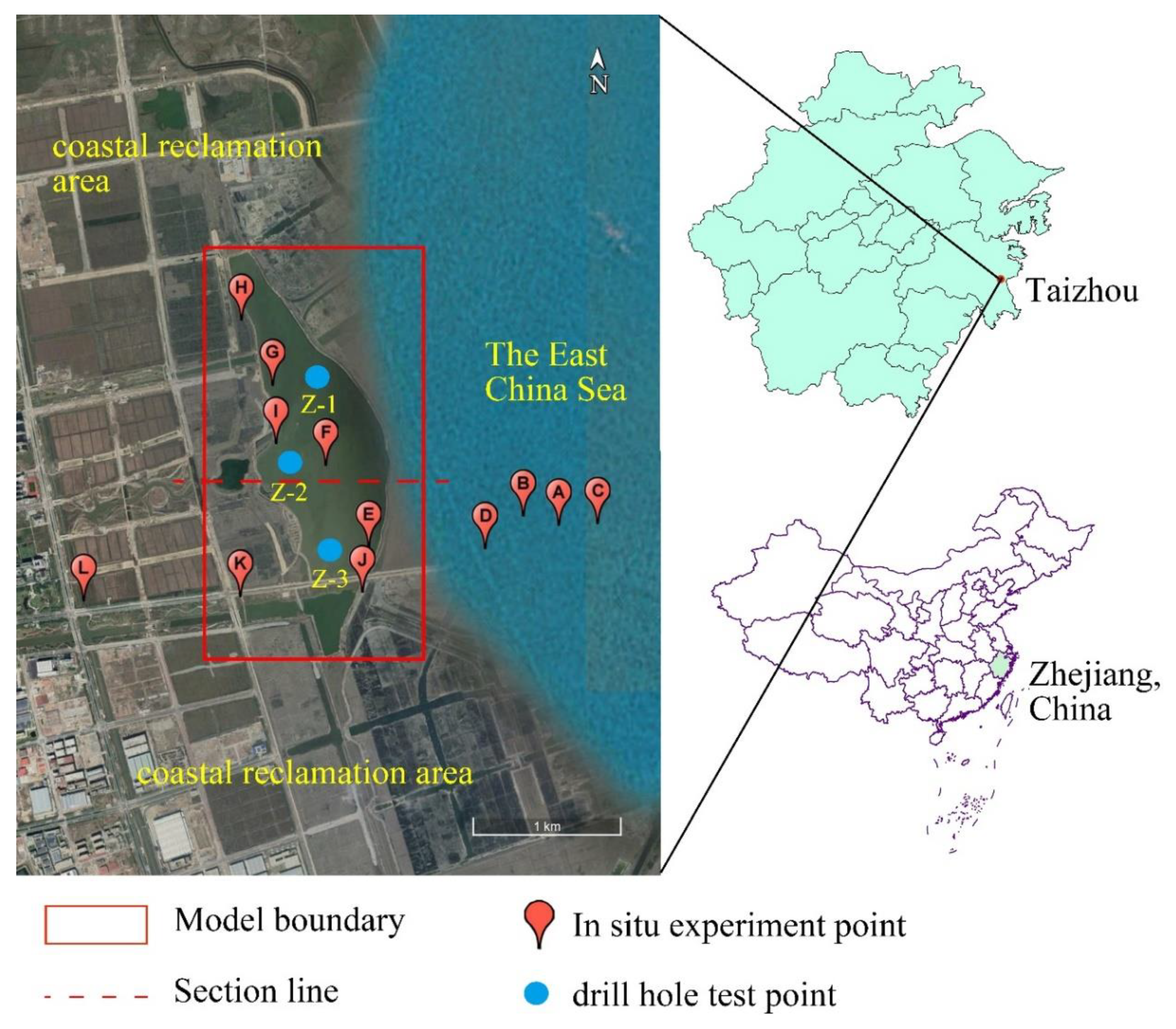
The following paragraphs describe the study area, the in situ test and experiment, and the numerical model. The hydraulic conductivity of the dredger filling area was obtained via an in situ standpipe experiment and slug test. Moreover, an experiment was designed to fit the molecular diffusion coefficient cooperating with a numerical model. The main model, which was conducted to predict salt release from the sediment–water interface, is described in detail using a mathematical model and model input. Two model scenarios considering water-exchange and lake stage, respectively, are also described in this section.

2.1. Study Area

Yuehu Lake is located west of the East China Sea in Southeast China, latitude 28°35′~28°36′ N and longitude 121°32′~121°33′ E (Figure 1). The study area encompasses approximately 3.63 km2. The Yuehu Lake is surrounded by a dredger filling area and the lake water comprises mostly sea water.
The salinity of the surrounding lake soil is 12 g/kg. The salinity levels of the sediments at different depths are shown in Table 1, which were obtained from drill-hole sampling collected at the blue dots in Figure 1 and tested by laboratory experiments. Three samples (Z-1, Z-2, Z-3) were obtained at each depth and the mean value was assigned to the numerical model. The sediment is composed of silt clay with low permeability. Because of the low-permeability dikes between the dredger fill area and the sea cutoff, the hydraulic connection between them, and the small runoff of the study area (about 2 m3/d), the effect of seawater flow on the lake is small and was ignored in the simulation. A cutoff wall was also placed around the lake, which restricted salt exchange between the surrounding soils and the lake.

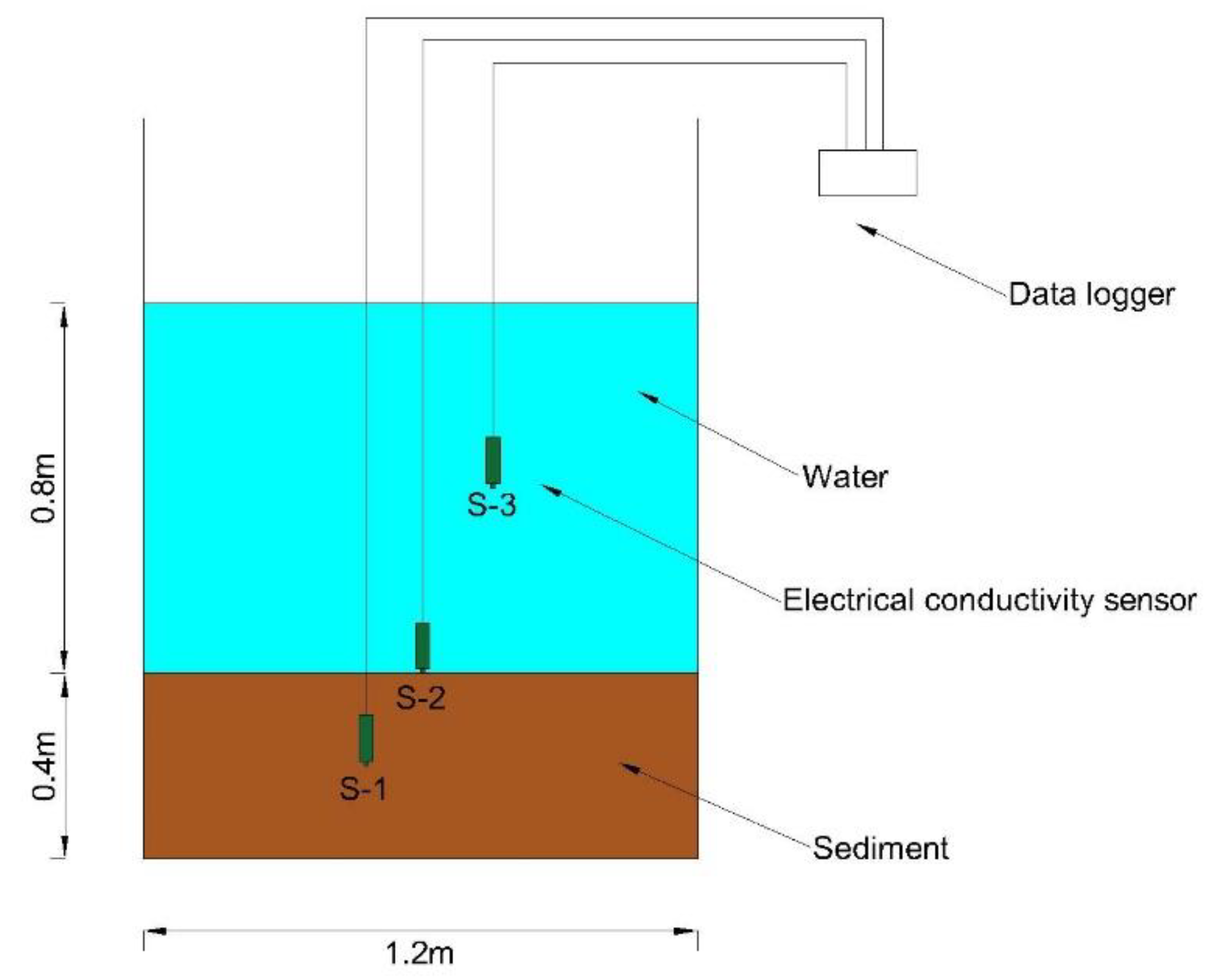
2.2. In Situ Tests and Experiments

An in situ standpipe experiment was used to obtain the vertical hydraulic conductivity (Kv) of the lake sediment. Twelve groups of experiments were conducted at Yuehu Lake and the results are shown in Table 2. The vertical hydraulic conductivity ranged from about 0.00063–0.00201 m/d. In addition, an in situ slug test was conducted to test horizontal hydraulic conductivity (Kh) and these results are shown in Table 3. The horizontal hydraulic conductivity ranged from about 0.0008–0.0024 m/d. The experiment sites covered the lake region and the dredger filling area, which are represented by the red balloon icons shown in Figure 1.
Both the standpipe experiments and slug tests lasted ten days. The mean values of the experimentally determined values were adopted as the hydraulic conductivity used in the numerical model. The vertical hydraulic conductivity was 1.26 × 10⁻³ m/d and the horizontal conductivity was 1.5 × 10⁻³ m/d. Both of these small values confirmed the low permeability of the soil in this area. The porosity of the soil can be calculated by the following equation:
θ = ( 1 ρ d ρ s ) × 100 % ,
where θ is the porosity of the soil (%), ρ d is the volume weight of the soil (N/cm3), and ρ s is the specific weight of the soil (null). Using the drill-hole samples from the sediment of lake, we tested the volume weight of the soil and the specific weight of the soil in the laboratory. We tested ten groups of samples and used the average value. The average porosity of the sediment was 0.3, based on laboratory testing. An experiment was designed to fit the molecular diffusion coefficient by fitting the experimental results using a numerical model calibration. The experimental apparatus is shown in Figure 2. The soil used in the experiment consisted of undisturbed samples collected from Yuehu Lake sediments. The lake bottom silt was placed in a big bucket 1.8 m in height with a 1.2 m diameter. The thickness of the lake bottom silt was 0.4 m, covered by 0.8 m of water. Three electrical conductivity sensors were installed in the bucket. S-1 was used to measure the electrical conductivity of the soil. It had a graphite electrode, which could be inserted into the soil directly. S-2 and S-3 measured the electrical conductivity of the solution through a titanium electrode. S-1 was located at the middle of the lake bottom silt, 0.2 m from the bucket bottom, S-2 was located at the interface of the silt and water, and S-3 was located in the middle of the water, 0.8 m from the bucket bottom. All sensors were connected to a data logger, which automatically recorded data. The water level was kept constant and interference of external force factors like wind influence were minimized by sealing the top of bucket to ensure salt was released from the sediment only via molecular diffusion, or as much as possible. The experiment lasted 900 h and the data were recorded hourly.

2.3. Mathematical Model

The mathematical representation of the homogeneous and anisotropy groundwater flow model can be described as
x ( K h h x ) + y ( K h h y ) + z ( K v h z ) Q = 0 ,
where K h is the horizontal hydraulic conductivity (m/d), K v is the vertical hydraulic conductivity (m/d), h is the water head (m), and Q is the volumetric flux per unit volume and represents sources or sinks of water (1/d). Equation (1), taken together with boundary and initial conditions, constitutes the groundwater flow model.
Solute (namely salt) transport in porous media is represented by the advection–dispersion equation between sediment and lake water and is given by the following mass conservation equation:
div ( θ D · C ) θ v · C = ( θ C ) t ,
where θ is the effective porosity (%), D is the molecular diffusion coefficient (m2/d), v is the actual average flow velocity (m/d), C is the salt concentration of the sediment or lake water (g/L), and t is time (d).
At the sediment and lake interface, the sediment and lake salt concentrations are usually considered equivalent. The governing equation is described by the following:
( C 1 v D 1 C 1 ) = ( C 2 v D 2 C 2 ) ,
where C 1 and C 2 are the salt concentrations of the sediment and lake water (g/L), and D 1 and D 2 are the molecular diffusion coefficients of salt in the sediment and lake water (m2/d).

2.4. Model Input

The governing equations of groundwater flow and salt transport (Equations (1) and (2)) were both solved numerically using the finite difference method based on commercial software (GMS 10.0). The MODFLOW and MT3DMS modules were used to simulate groundwater seepage and the salt-release process on the sediment–water interface, respectively.
The study area was divided into 20 cells in the x-direction and 80 cells in the y-direction; each cell was 34 × 67 m. Vertically, the study area was divided into 28 layers. The Yuehu Lake water was divided into 16 layers with vertical nodal spacing of 0.25 m. The thickness of the sediment considered in this simulation was 3 m, which was divided into 12 layers.
Boundary conditions of the study area were set as the Dirichlet boundary condition and we assumed that the water head was constant during the simulation period. The initial salt concentration of the lake water was 0.5 g/L. The initial salt concentrations of the sediment were 10 g/kg (0–1 m), 16 g/kg (1–1.5 m), and 14 g/kg (1.5–3 m); this was based on data from drill-hole sampling tests, as shown in Table 1. At the interface of the lake water and the sediment, the salt concentrations for both were considered the same.
Another model was built to fit the molecular diffusion coefficient, which simulated the experiment mentioned above. This model was considered to be one-dimensional because of the homogeneous isotropic soil used in the experiments, and the electrical conductivity sensors were set to the one-dimension form. A water column of 0.8 m was divided into 160 cells, each of which was 0.05 × 0.12 m and the sediment was divided into 80 cells. The hydraulic conductivity and average porosity of the sediment were the same as the Yuehu Lake model.

2.5. Model Scenarios

Salt-release rates usually decrease with time as the concentration gradient decreases between the lake water and sediment. To promote salt release from the sediment, a water-exchange method, involving the replacement of salt water in Yuehu Lake with freshwater, was adopted. Different water-exchange periods (30 d, 60 d, 90 d, 216 d, 360 d) were considered. In these simulations, the time spent in operation of water-exchange was ignored and the simulation period was 1080 days. The elevation of the lake stage was set to be stable and measured to be 2 m tall with an average lake water depth of 4 m.
Two different lake stages of 2.0 m and 1.0 m were set for the model prediction and the average corresponding lake water depths were 4.0 m and 3.0 m, respectively. The simulation period was 3600 d. To clearly observe the influence of the lake stage on the variation of the lake water salinity, no water-exchange scenario was adopted.

3. Results and Discussion

Model calibration is often also called history matching. When the ultimate goal of model calibration is not merely to calibrate a model, but rather to optimize unknown parameters in that model, the process is often called parameter estimation or parameter inversion. Salinity distribution at the end of the simulation period under water-exchange scenarios and lake stage scenarios are illustrated in this section.

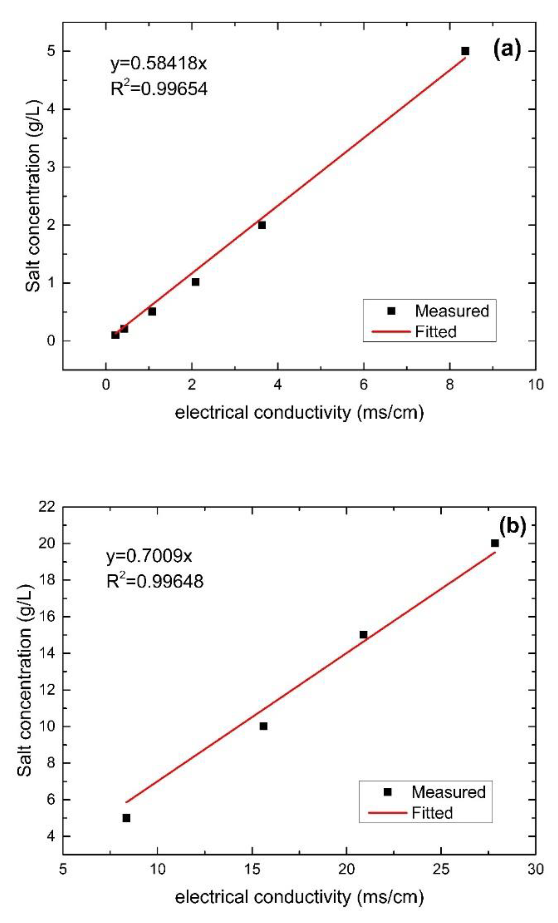
3.1. Parameter Inversion

Before the numerical simulation, a standard curve of salinity vs. electrical conductivity was obtained via laboratory experiments at 25 °C. This experiment used the same sensors as the experiment which fit the molecular diffusion coefficient. Because the relationship between salt concentration and electrical conductivity differs with salt concentration ranges, standard curves were drawn for the two salt concentration ranges (0–5 g/L and 5–20 g/L); both of these are shown in Figure 3.
The numerical model was calibrated based on monitoring experimental data to fit the molecular diffusion coefficient. Figure 4 shows the measured and calculated salinity variation profiles at various times. The experimental data were calibrated to 25 °C, and the electrical conductivity data were transformed into a salt concentration by fitting the conductivity data onto the standard salinity vs. electrical conductivity curve.
The missing data between 330–367 h was caused by a data logger malfunction. The fitting effect of the calculated and measured values was judged by root mean squared error (RMSE) and correlation coefficient (R) during this simulation. The fitting effect negatively correlated with the root mean squared error (RMSE) and positivity correlated with the correlation coefficient (R). The RMSEs of measured data and simulated results at the water, interface, and sediment were 0.03848 g/kg, 0.07018 g/kg, and 0.07999 g/kg, respectively, with correlation coefficients of 0.98794, 0.93318, and 0.97964 respectively. The low RMSE values and high R values indicated a good fit. The simulated salt concentrations at different depths matched the transient calibration salinity target. The measured data in the sediment–water interface was higher than the simulated value observed the early stage of the simulation but became consistent as the salt concentration stabilized. Based on the inversion of the experiment through simulation, the molecular diffusion coefficients of salt used in this study were obtained (1.39 × 10⁻⁹ m2/s in sediment and 4.17 × 10⁻⁹ m2/s in water). Li and Gregory [8] measured the diffusion coefficients of different ions in seawater at an infinite dilution; the diffusion coefficient of the chloride ion is 2.03 × 10⁻⁹ m2/s.

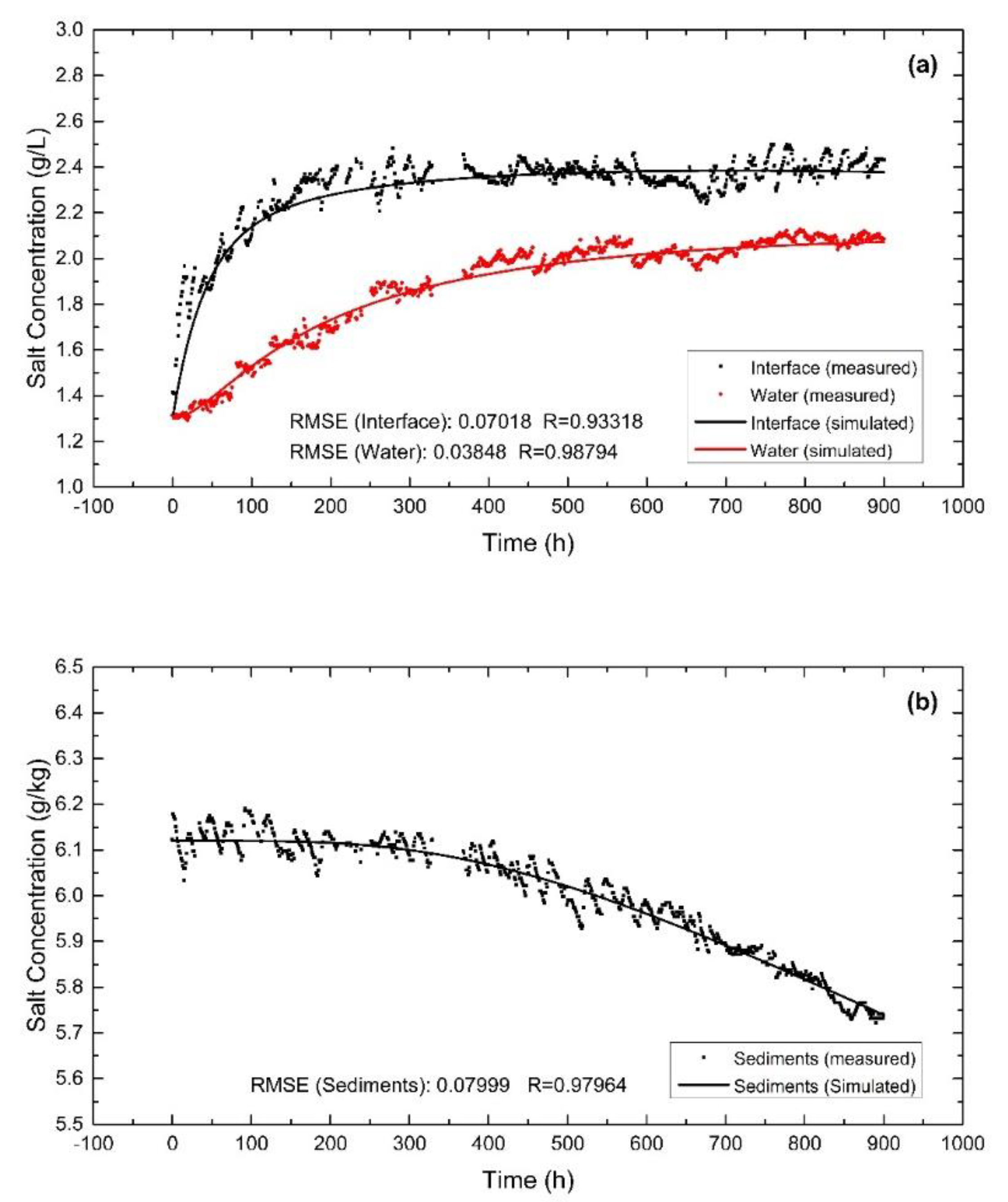
3.2. Model Validation

The current project adopted the 90 d water-exchange scenario. Measured data of salinity at different depth in Yuehu Lake during the water-exchange period (the 90th and 180th day) were used to validate the numerical model. The comparison between the simulated and measured values showing the model validation results are listed in Table 4.
The RMSEs of the measured data and simulated results were 0.13491 g/L and 0.09316 g/L at the end of the first and second water-exchange periods, respectively, with correlation coefficients of 0.99892 and 0.99838, respectively, which indicated a good fit. Measured data from 0.5 m to 1 m were unchanged compared with the initial value, which showed that the influence scope of the salt release from sediment was less than 0.5 m. The measured data were a little smaller than the simulation results, which may be the reason why miscibility of lake water exists in reality. The low RMSE values and high R indicated that our model could be used to predict salt release from sediment under a water-exchange scenario.

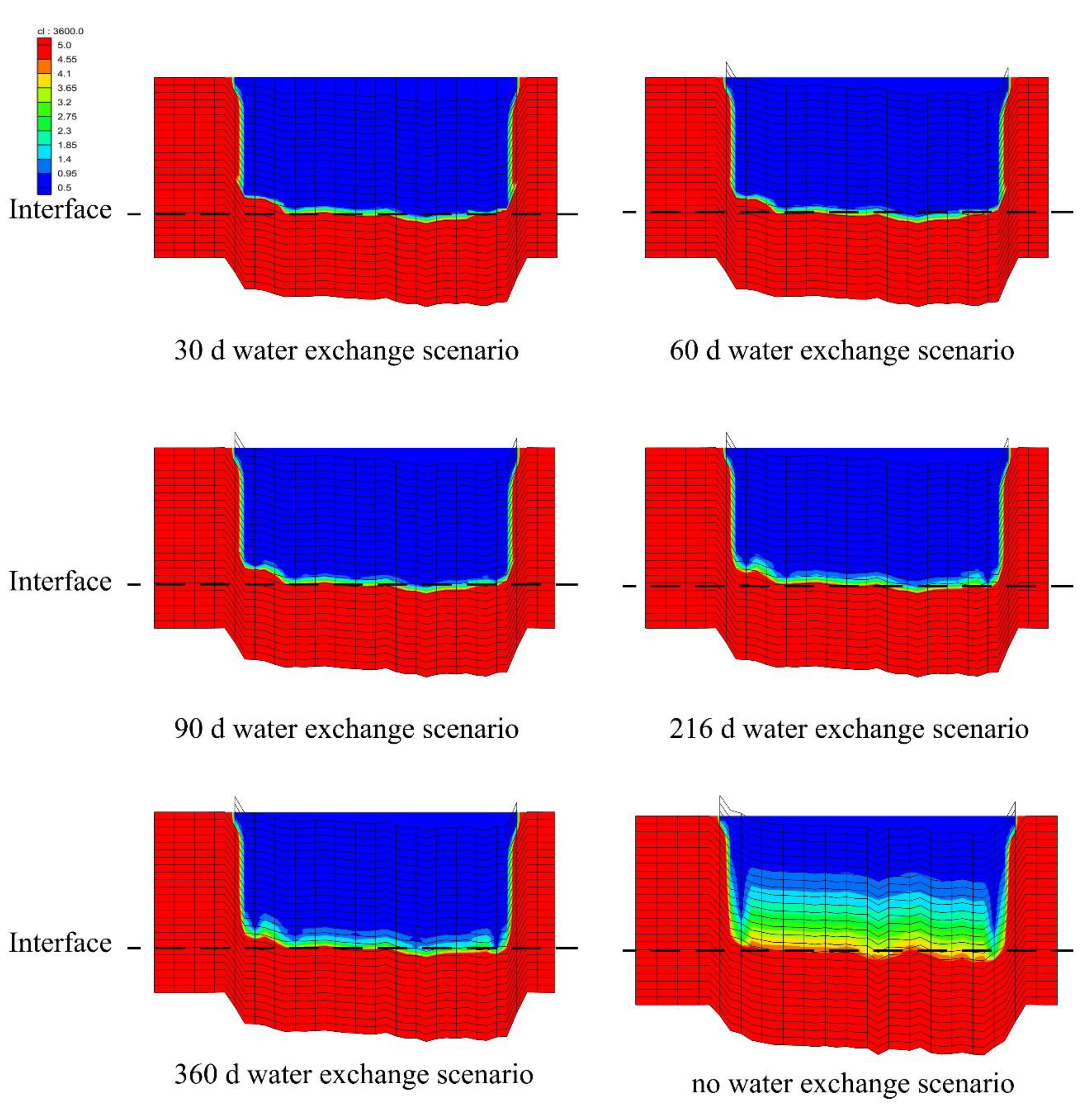
3.3. Salinity Distribution under Water-Exchange Scenarios

Figure 5 shows the salinity distribution in the water and sediment surfaces of the section shown in Figure 1 at the end of simulation period under six water-exchange scenarios for Yuehu Lake. These results indicated that more frequent water-exchange maintained a lower salt concentration near the sediment–water interface. At the same time, more frequent water-exchange also promoted salt release from the sediment. The simulation results suggested that a 30 d water-exchange scenario had the greatest impact on expediting salt release from the sediment, whereas no water-exchange scenario had the highest sediment surface salt concentration at the end of the simulation period. Water-exchange effectively reduced the salt concentration at the sediment surface and controlled surface water salinization.

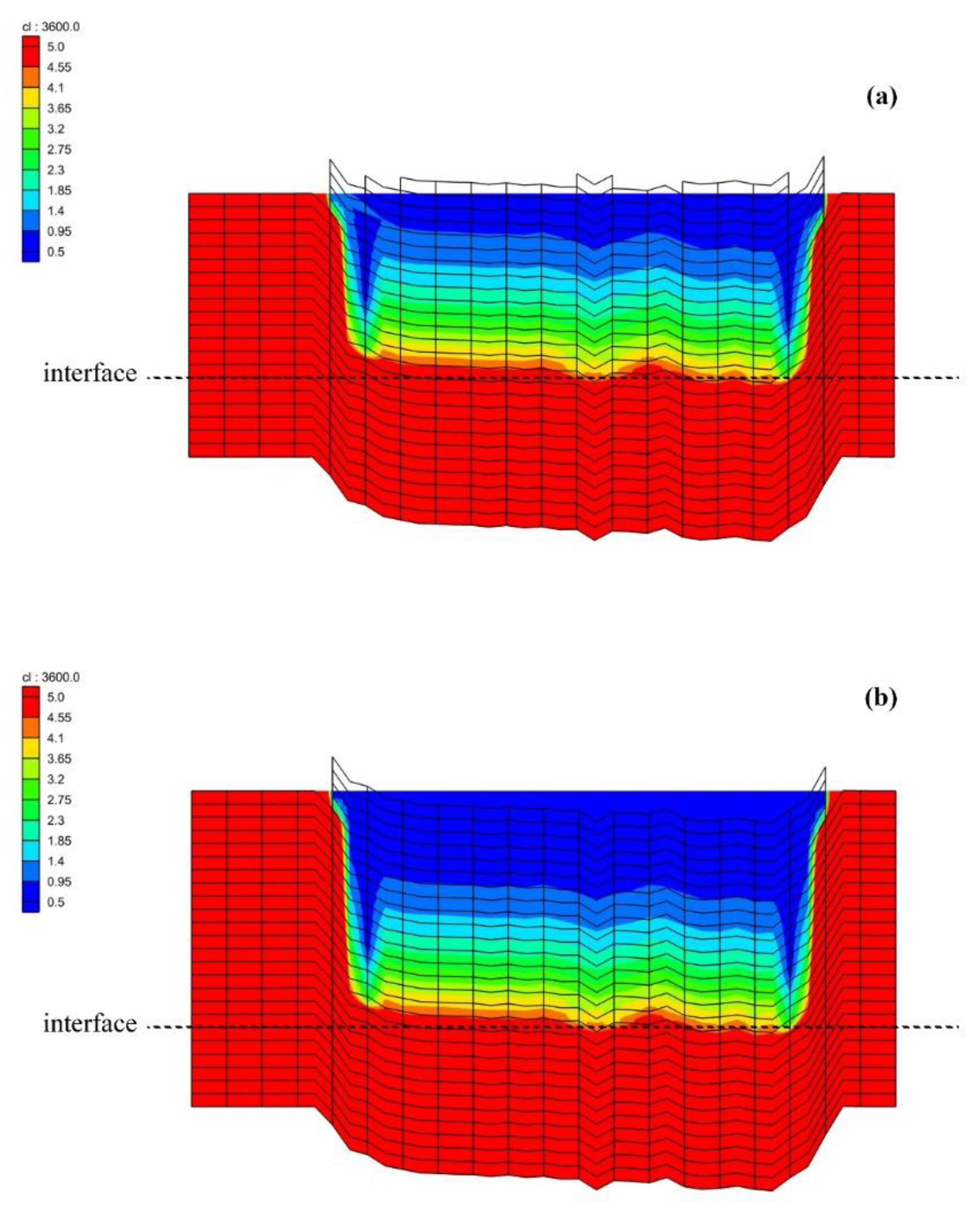
3.4. Salinity Distribution under Lake Stage Scenarios

Figure 6 shows the salt concentration distribution for the lake stages of 2.0 m and 1.0 m at the end of the simulation period. The salt capacity of water is related to salt solubility, therefore, salt release is impeded when the salt capacity of the water is maximized and the concentration gradient is too small to advance additional salt release. The salt concentration distributions for the lake stages of 2.0 m and 1.0 m were nearly identical, meaning that salt release from the sediment was not impeded and the salt capacity of the lake water was not maximized during the simulation period. For low-permeability areas like this one, the efficiency of sediment salt release related primarily to the water/sediment concentration gradient. Water thickness had little influence on sediment salt release before the salt capacity of the water was maximized. Salt release from sediments is a long, slow process in low-permeability areas.

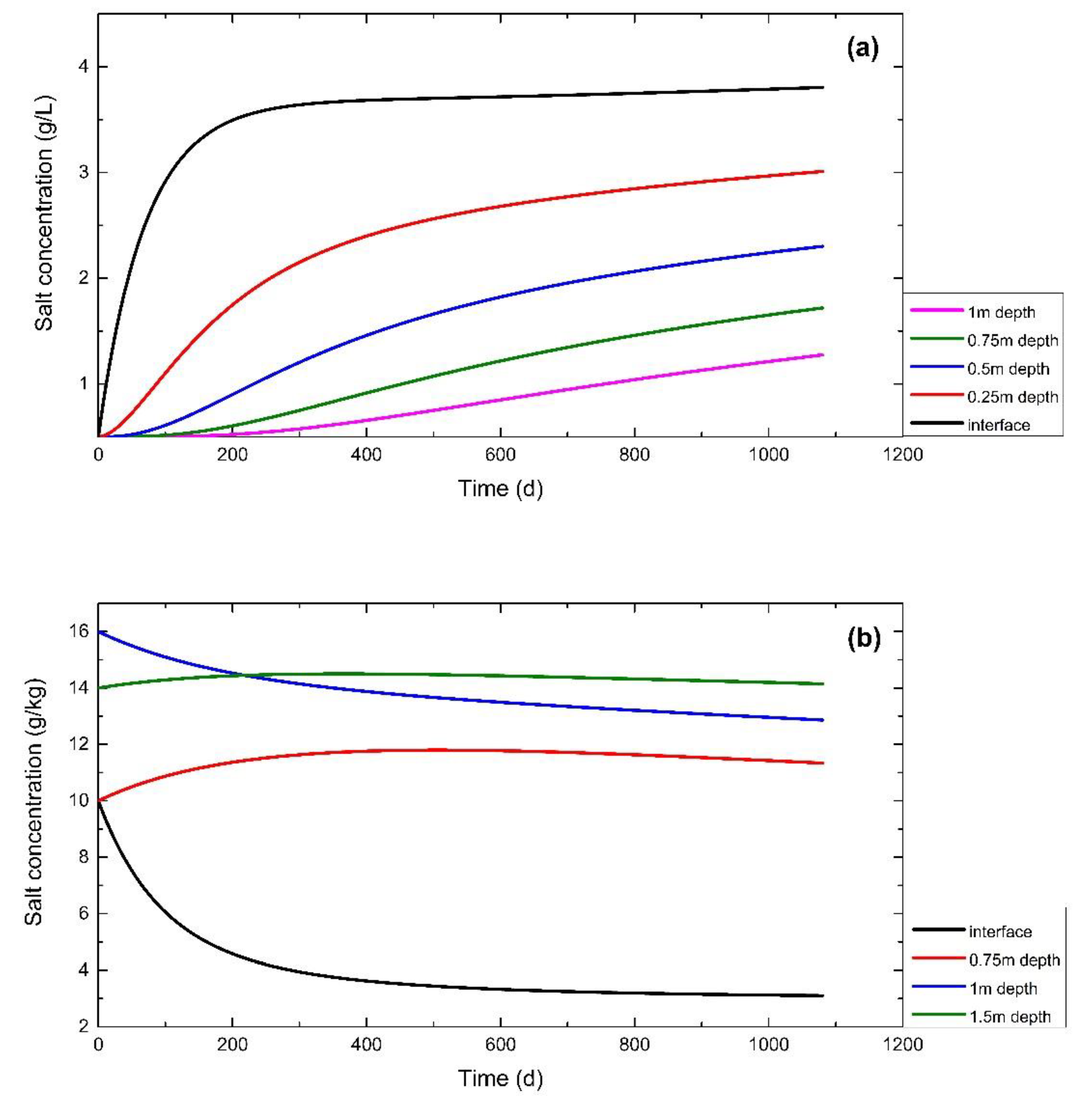
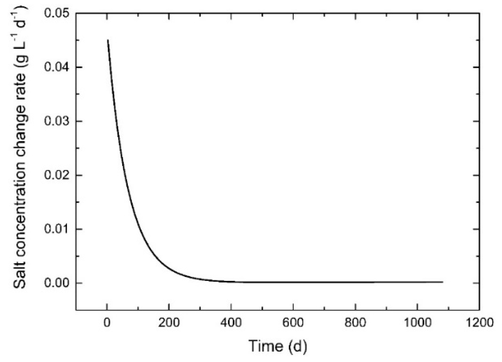
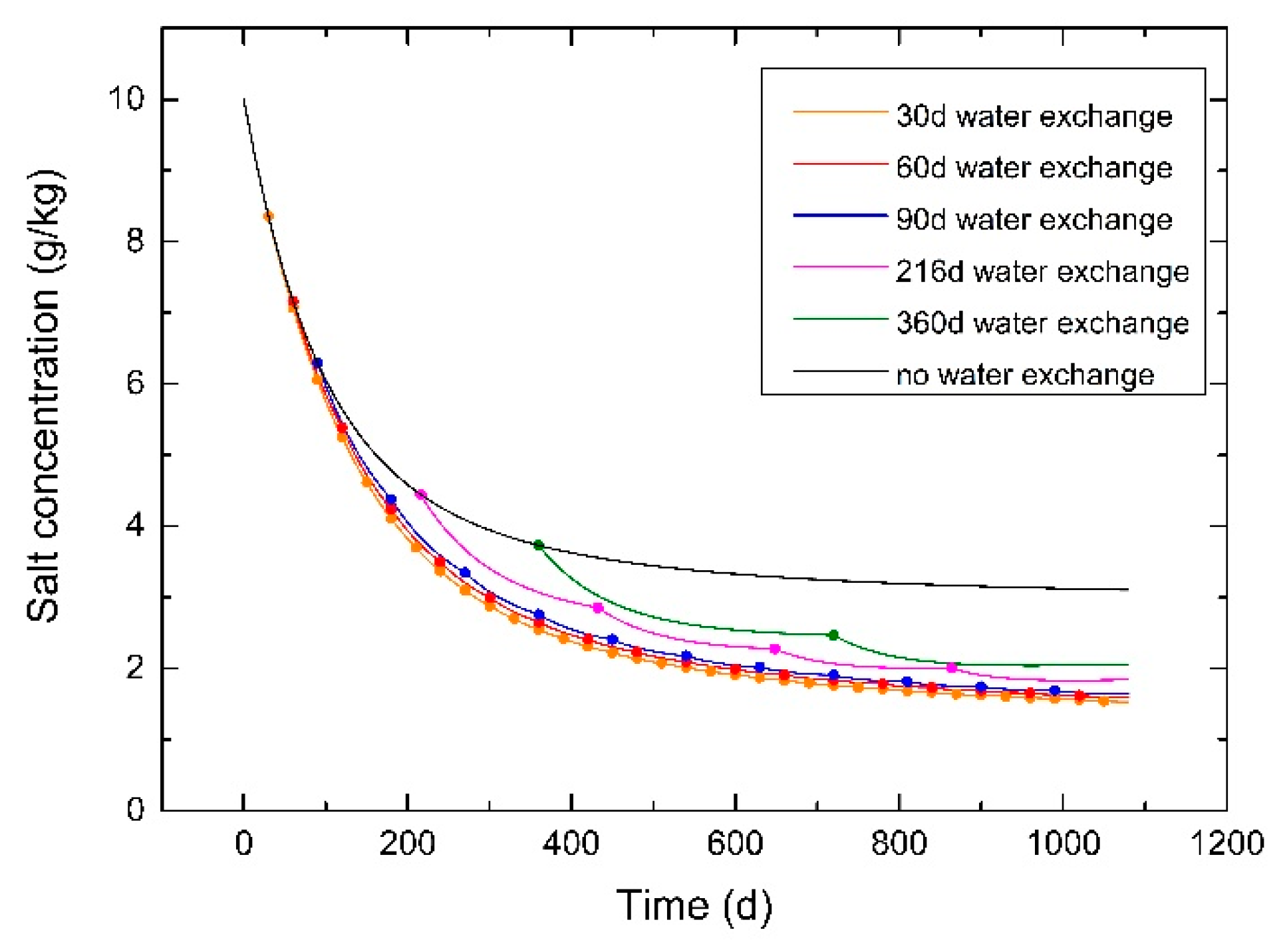
3.5. Effect of Period of Water-Exchange

Water-exchange effectively accelerates the process of salt release from sediment and replaces salt water with freshwater in a timely fashion. The variation in the salt concentration change rate shows the exchange rate between the sediment and water.
Figure 7 shows the average salt concentration profile of the sediment at 0.75 m, 1 m, and 1.5 m at the interface and water at 1 m of the interface under no water-exchange scenario. As shown in the figure, the average salt concentration of the lake water increased with increasing depth; the rate of increase gradually slowed as a function of distance from the interface. The average lake water salt concentration at the interface increased rapidly in the first 100 d and represented a 500% increase of the initial concentration. The average sediment salt concentration tended to decrease, with the average sediment salt concentration at the interface approximately 72% lower than the initial concentration. The salt concentration of the sediment below 1.5 m was almost unchanged during the simulation period because of the long distance from the interface and the small concentration gradient with adjacent layers. The average concentration of the sediment at 0.75 m increased initially but decreased with time because of the supply from the lower layer (1–1.5 m) with a higher salt concentration, thereby showing that molecular diffusion was also obvious in the sediment. The average salt concentration of the sediment at 1.5 m increased slightly and tended to be stable, which showed that salt release from the top layer (1–1.5 m) could be both upward and downward.
Figure 8 proves that the salt concentration change rate in the water layer (0–0.25 m) decreased gradually with time. The variation of water salinity was primarily driven by the molecular diffusion of salt from the sediment, and the release rate of the sediment slowed down as the water salinity increased. On the 360th day, the change rate stabilized, illustrating that the salt concentrations on both sides of the interface reached similar concentrations and the system equilibrated. A lower salt concentration in water maintained a relatively high concentration gradient with the sediment and kept salt release at a high-speed state, so water-exchange scenarios were considered.
Figure 9 shows the average salt concentration at the sediment surface at 30 d, 60 d, 90 d, 216 d, and 360 d and no water-exchange scenario. The effect of salt release of these five water-exchange scenarios was better than no water-exchange scenario. The average salt concentration at the sediment surface was 3.10 g/kg after 1080 days with the no water-exchange scenario, while the sediment salinities were 1.52 g/kg, 1.58 g/kg, 1.64 g/kg, 1.84 g/kg, and 2.07 g/kg for the five water-exchange scenarios, respectively. The effect of salt release significantly improved, which achieved the purpose of sediment salinity reduction to control surface water salinization. The average salt concentrations of water-exchange at 30 d, 60 d, and 90 d were approximately 50% lower than the no water-exchange scenario at the end of the simulation period. The nodes in the figure represent the water-exchange time and the number of nodes corresponds to the number of water-exchange steps under each scenario. In all of the water-exchange scenarios, the salinity of the sediment decreased. The ending salt concentrations after the 30 d and 360 d water-exchange scenarios were 1.52 g/kg and 2.07 g/kg, respectively; the salt concentrations for the other water-exchange scenarios were between those two values. In the first three scenarios (30 d, 60 d, and 90 d), the variation lines of salt concentration were smooth. In these three changing water periods, the water salinity stayed at a relative low value during the entire simulation period, and the salt-release rate was relatively fast because of the high concentration gradient between the water and sediment, so there were no obvious changes on the graph corresponding to water-exchange. On the contrary, catastrophe points occurred when the water-exchange scenario was 216 d and 360 d; these clear changes were caused by a sudden increase in the salt-release rate during water-exchange, before which the concentration gradient between the water and sediment decreased and remained at a low level. Around the 90th day, there was a marked decline in the sediment salt-release rate which was due to the relatively high salt concentration in the lake water. Water-exchanges of 30 d, 60 d, and 90 d maintained high salt-release rates in the sediment. Though changing the water every 30 d was the best, it was only 3% and 7% better than 60 d and 90 d respectively. More frequent water-exchanges could achieve the best effect, but this advantage is small compared to relatively low frequencies, which could also maintain a fast rate of salt release. The results showed that a water-exchange period of 90 d maintained a relatively fast salt-release rate and conserved water resources due to fewer water-exchange steps.

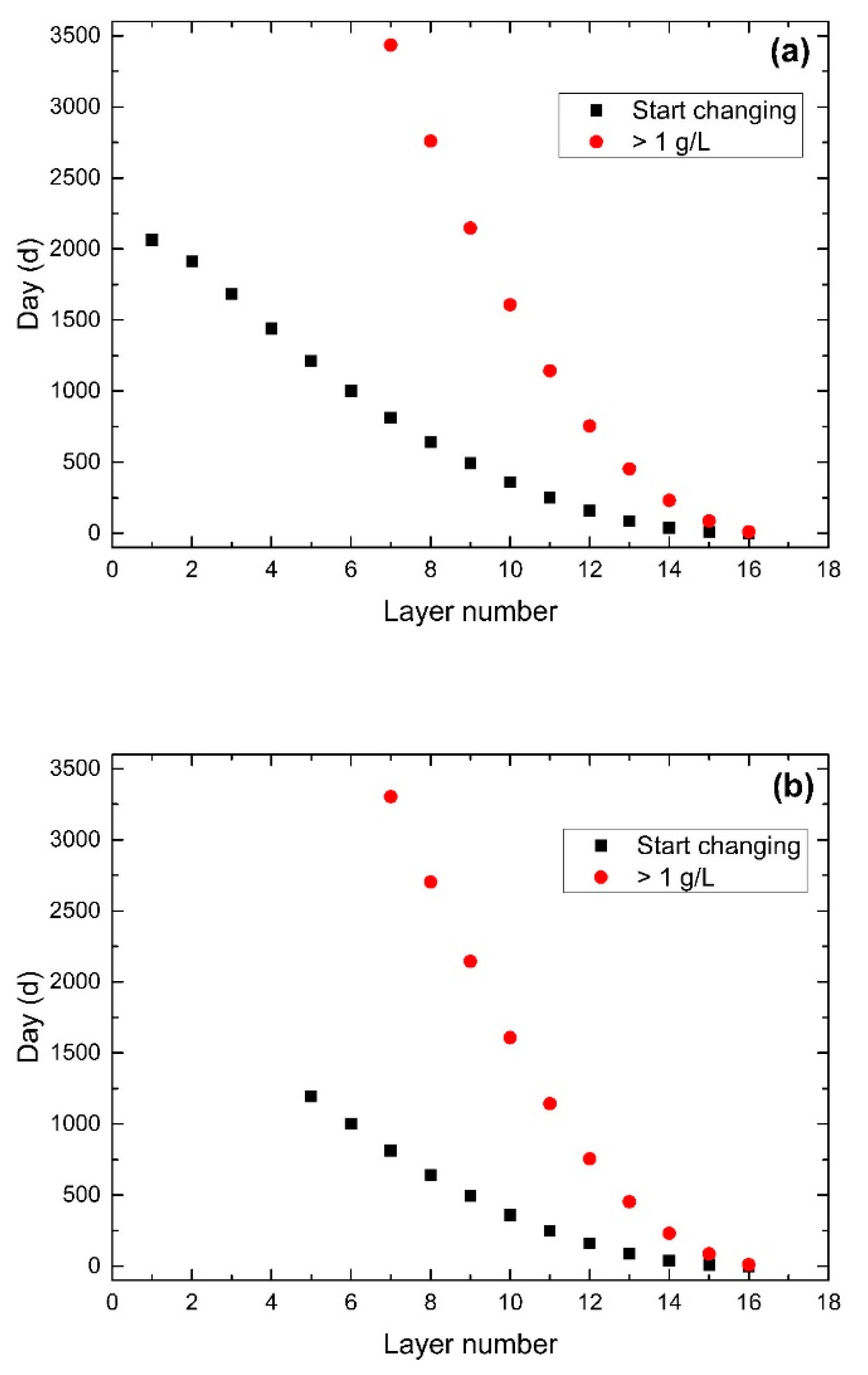
3.6. Effect of Lake Stage

Figure 10 shows the change rate in salt concentration at the sediment surface with no water-exchange but with different lake stages. Though the two scenarios had different lake stages, the salt concentration differences in the sediment were nearly identical with slight differences, which caused the salt concentration change rates under the two scenarios to be almost the same and appear as overlapped lines in Figure 10. The salt concentration change rate became stable around the 500th day, before which the salt released relatively quickly, then gradually stabilized to 3 g/kg. The average salt concentration of the lake water increased during the simulation period, which meant salt release took place even when the average salt concentration of the sediment stabilized, during which the supply from the lower layer and that released from the upper layer is equilibrated. Currently, the average salt concentrations of the water and sediment were similar; the concentration of the former was slightly lower than the latter, which caused subtle molecular diffusion.
The salinity index of freshwater in a human-living area is less than 1 g/L. The time at which the change started and became greater than 1 g/L of the average salt concentration in water at each layer is shown in Figure 11. The water depth was divided into 16 layers, with the 16th (0–0.25 m from the interface) layer adjacent to the sediment. From that layer to the 6th (2.5–2.75 m) layer, the time at which change time started was the same in both scenarios. Salt concentrations began to change on day 1194 under the lake stage of 1.0 m, 18 days earlier than the lake stage 2.0 m scenario at the 5th layer. The time taken for the average salt concentration to become greater than 1 g/L was same as these two scenarios from the 16th (0–0.25 m) to the 10th (1.5–1.75 m) layer. The times taken for the average salt concentration to become greater than 1 g/L of the 9th (1.75–2 m), the 8th (2–2.25 m), and the 7th (2.25–2.5 m) layers were the 2145th, the 2703rd, and the 3303rd day under the 1 m scenario, which are 3, 57, and 132 days earlier than 2 m scenario. The average salt concentrations of the layers above the 7th layer was not greater than 1 g/L at any time during the simulation period. In short, the influence of salt release from the sediment to water increased with time, and the salt capacity of the lake was much higher than the amount of salt released to the lake. Because of the low molecular diffusion from the sediment, salt transport was weak. Salt in the first layer rapidly released into the water, so the salt concentration of the first layer stayed relatively low during the simulation period. Though the supply from the lower layer reached the first layer, the supply also released quickly into the water and reached equilibrium.

4. Conclusions

The salinity index of freshwater in human-living areas is generally less than 1 g/L. Sediments with high salinity can cause the degradation of water through salt release in coastal reclamation area. To clarify the salt-release process and provide an efficient method to dispose of sediments with high salinity, a numerical model was established to simulate salt transport across the interface between sediment and water in a low-permeability area. In situ tests and physical experiments were conducted to calculate hydraulic parameters and observe variations in salt concentrations in sediment and water. Numerical models were used to calibrate molecular diffusion coefficients and predict salt-release processes at the sediment–water interface in Yuehu Lake, China. Different water-exchange scenarios were considered and compared in the model. The results showed that the sediment released salt more slowly and became stable once the salt concentration in water reached a certain level. The salt concentration of the water increased rapidly and stabilized after approximately one year. Though a faster frequency of water-exchange controlled sediments and water salinization more effectively, water-refreshing rates more frequent than 90 d were similarly as effective as a 90 d water-exchange cycle. Refreshing the water every 90 days resulted in the sediment releasing salt at a relatively rapid rate. Two types of lake stage were considered and showed that the influence of water depth on salt release from sediment was not apparent before the salt capacity of the water was reached. The influence of the salt release at each layer was related to the distance from the interface and the immersion time. The salt concentration of the water increased rapidly within 0.5 m from the interface and reached 1 g/L after 90 days. Layers of water more than 2.5 m from the interface did not reach 1 g/L during the simulation periods. When the salt concentration at the sediment surface stabilized, a salt-release process also existed; at that time, the supply from the lower layers was comparable to the release into the water to reach equilibrium. In summary, in order to ensure that lake water quality meets ecological needs in coastal reclamation areas, we propose a new method involving water-exchange to dispose of sediments with high salinity. We compared several scenarios under different water-exchange periods and lake stages during the implement of water-exchange, and found an effective and resource-saving scheme which can be used as a reference for the treatment of sediments with high salinity in the future.

Author Contributions

J.W. and Z.C. conceived and designed the experiments; W.L., Y.Z., and D.Y. conducted the experiments; W.L. and R.L. analyzed the data; W.L. and Z.C. established the numerical model; W.L. and Y.Y. wrote the paper; J.W. edited the paper.

Funding

This research received no external funding.

Acknowledgments

This research was financially supported by the National Key R&D Program of China (Grant Nos. 2016YFC0401801 and 2016YFC0402800) and the Fundamental Research Funds for the Central Universities (Grant No. 2018B58514). We are grateful to the editor and the two anonymous reviewers whose invaluable suggestions have led to significant improvement in this manuscript.

Conflicts of Interest

The authors declare no conflict of interest.

References

  1. Antonellini, M.; Mollema, P.N. Impact of groundwater salinity on vegetation species richness in the coastal pine forests and wetlands of Ravenna, Italy. Ecol. Eng. 2010, 36, 1201–1211. [Google Scholar] [CrossRef]
  2. Abarca, E.; Karam, H.; Hemond, H.F.; Harvey, C.F. Transient groundwater dynamics in a coastal aquifer: The effects of tides, the lunar cycle, and the beach profile. Water Resour. Res. 2013, 49, 2473–2488. [Google Scholar] [CrossRef]
  3. Badaruddin, S.; Werner, A.D.; Morgan, L.K. Water table salinization due to seawater intrusion. Water Resour. Res. 2015, 51, 8397–8408. [Google Scholar] [CrossRef]
  4. Mccarthy, T.S. Groundwater in the wetlands of the Okavango Delta, Botswana, and its contribution to the structure and function of the ecosystem. J. Hydrol. 2006, 320, 264–282. [Google Scholar] [CrossRef]
  5. Mondal, N.C.; Singh, V.P. Hydrochemical analysis of salinization for a tannery belt in Southern India. J. Hydrol. 2011, 405, 235–247. [Google Scholar] [CrossRef]
  6. Jurinak, J.J.; Whitmore, J.C.; Wagenet, R.J. Kinetics of salt release from a saline soil. Soil Sci. Soc. Am. J. 1977, 41, 721–724. [Google Scholar] [CrossRef]
  7. Domenico, P.A.; Mifflin, M.D. Water from low-permeability sediments and land subsidence. Water Resour. Res. 1965, 1, 563–576. [Google Scholar] [CrossRef]
  8. Robinson, C.; Gibbes, B.; Li, L. Driving mechanisms for groundwater flow and salt transport in a subterranean estuary. Geophys. Res. Lett. 2006, 33, L03402. [Google Scholar] [CrossRef]
  9. Wei, X.; Qun, L.; Shusheng, G.; Zhiming, H.; Hui, X. Pseudo threshold pressure gradient to flow for low permeability reservoirs. Explor. Dev. 2009, 36, 232–236. [Google Scholar] [CrossRef]
  10. Gonneea, M.E.; Mulligan, A.E.; Charette, M.A. Climate-driven sea level anomalies modulate coastal groundwater dynamics and discharge. Geophys. Res. Lett. 2013, 40, 2701–2706. [Google Scholar] [CrossRef]
  11. Neuzil, C.E. Groundwater flow in low-permeability environments. Water Resour. Res. 1986, 22, 1163–1195. [Google Scholar] [CrossRef]
  12. Neuzil, C.E. How permeable are clays and shales? Water Resour. Res. 1994, 30, 145–150. [Google Scholar] [CrossRef]
  13. Remenda, V.H.; Kamp, G.; Cherry, J.A. Use of vertical profiles of δ18O to constrain estimates of hydraulic conductivity in a thick, unfractured aquitard. Water Resour. Res. 1996, 32, 2979–2987. [Google Scholar] [CrossRef]
  14. Hendry, M.J.; Wassenaar, L.I. Implications of the distribution of δD in pore waters for groundwater flow and the timing of geologic events in a thick aquitard system. Water Resour. Res. 1999, 35, 1751–1760. [Google Scholar] [CrossRef]
  15. Rubel, A.P.; Sonntag, C.; Lippmann, J.; Pearson, F.J.; Gautschi, A. Solute transport in formations of very low permeability: Profiles of stable isotope and dissolved noble gas contents of pore water in the Opalinus Clay, Mont Terri, Switzerland. Geochim. Cosmochim. Acta 2002, 66, 1311–1321. [Google Scholar] [CrossRef]
  16. Wanner, P.; Hunkeler, D. Carbon and chlorine isotopologue fractionation of chlorinated hydrocarbons during diffusion in water and low permeability sediments. Geochim. Cosmochim. Acta 2015, 157, 198–212. [Google Scholar] [CrossRef]
  17. Lebbe, L.; Meir, N.V. Hydraulic conductivities of low permeability sediments inferred from a triple pumping test and observed vertical gradients. Groundwater 2000, 38, 76–88. [Google Scholar] [CrossRef]
  18. Cey, B.D.; Barbour, S.L.; Hendry, M.J. Osmotic flow through a Cretaceous clay in southern Saskatchewan, Canada. Can. Geotech. J. 2001, 38, 1025–1033. [Google Scholar] [CrossRef]
  19. Liu, H.H. Non-Darcian flow in low-permeability media: Key issues related to geological disposal of high-level nuclear waste in shale formations. Hydrogeol. J. 2014, 22, 1525–1534. [Google Scholar] [CrossRef]
  20. Papadokostaki, K.G.; Petrou, J.K. Combined experimental and computer simulation study of the kinetics of solute release from a relaxing swellable polymer matrix. I. Characterization of non-fickian solvent uptake. J. Appl. Polym. Sci. 2004, 92, 2458–2467. [Google Scholar] [CrossRef]
  21. Ling, J. Characteristics and mechanism of low permeability clastic reservoir in Chinese petroliferous basin. Acta Sedimentol. Sin. 2004, 22, 13–18. [Google Scholar]
  22. Li, Y.H.; Gregory, S. Diffusion of ions in seawater and deep sea sediments. Geochim. Cosmochim. Acta 1974, 88, 708–714. [Google Scholar]
  23. Van Rees, K.C.J.; Sudicky, E.A.; Rao, P.S.C.; Reddy, K.R. Evaluation of laboratory techniques for measuring diffusion coefficients in sediments. Environ. Sci. Technol. 1991, 25, 1605–1611. [Google Scholar] [CrossRef]
  24. Barone, F.S.; Rowe, R.K.; Quigley, R.M. Estimation of chloride diffusion coefficient and tortuosity factor for mudstone. J. Geotech. Eng. 1992, 118, 1031–1045. [Google Scholar] [CrossRef]
  25. Hendry, M.J.; Barbour, S.L.; Boldt-Leppin, B.E.J.; Reifferscheid, L.J.; Wassenaar, L.I. A comparision of laboratory and field based determinations of molecular diffusion coefficients in a low permeability geologic medium. Environ. Sci. Technol. 2009, 43, 6730–6736. [Google Scholar] [CrossRef] [PubMed]
  26. Zhou, D.; Jia, L.; Kamath, J.; Kovscek, A.R. Scaling of counter-current imbibition processes in low-permeability porous media. J. Pet. Sci. Eng. 2002, 33, 61–74. [Google Scholar] [CrossRef]
  27. French, J.A.; Harley , B.M.; Neysadurai, A. Desalination of an Important Estuary. Environment Engineering, Process of the 1985 Specialty Conference; ASCE: New York, NY, USA, 1985; pp. 91–97. [Google Scholar]
  28. Johnson, R.L.; Cherry, J.A.; Pankow, J.F. Diffusive contaminant transport in natural clay: A field example and implications for clay-lined waste disposal sites. Environ. Sci. Technol. 1989, 23, 340–349. [Google Scholar] [CrossRef]
  29. Portielje, R.; Lijklema, L. Estimation of sediment-water exchange of solutes in Lake Veluwe, the Netherlands. Water Res. 1999, 33, 279–285. [Google Scholar] [CrossRef]
  30. Malusis, M.A.; Shackelford, C.D. Coupling effects during steady-state solute diffusion through a semipermeable clay membrane. Environ. Sci. Technol. 2002, 36, 1312–1319. [Google Scholar] [CrossRef]
  31. Heiss, J.W.; Michael, H.A. Saltwater-freshwater mixing dynamics in a sandy beach aquifer over tidal, spring-neap, and seasonal cycles. Water Resour. Res. 2014, 50, 6747–6766. [Google Scholar] [CrossRef]
  32. Mero, F.; Simon, E. The simulation of chloride inflows into Lake Kinneret. J. Hydrol. 1992, 138, 345–360. [Google Scholar] [CrossRef]
  33. Assouline, S. Estimation of lake hydrologic budget terms using the simultaneous solution of water, heat, and salt balances and a Kalman Filtering Approach: Application to Lake Kinneret. Water Resour. Res. 1993, 29, 3041–3048. [Google Scholar] [CrossRef]
  34. Hurwitz, S.; Lyakhovsky, V.; Gvirtzman, H. Transient salt transport modeling of shallow brine beneath a freshwater lake, the Sea of Galilee, Israel. Water Resour. Res. 2000, 36, 101–107. [Google Scholar] [CrossRef] [Green Version]
  35. Rimmer, A. The mechanism of Lake Kinneret salinization as a linear reservoir. J. Hydrol. 2003, 281, 173–186. [Google Scholar] [CrossRef]
  36. Papadokostaki, K.G. Combined experimental and computer simulation study of the kinetics of solute release from a relaxing swellable polymer matrix. II. Release of an osmotically active solute. J. Appl. Polym. Sci. 2004, 92, 2468–2479. [Google Scholar] [CrossRef]
  37. Siyal, A.A.; Skaggs, T.H.; Van Genuchten, M.T. Reclamation of saline soils by partial ponding: Simulations for different soils. Vadose Zone J. 2010, 9, 486–495. [Google Scholar] [CrossRef]
  38. Harte, P.T.; Konikow, L.F.; Hornberger, G.Z. Simulation of solute transport across low-permeability barrier walls. J. Contam. Hydrol. 2006, 85, 247–270. [Google Scholar] [CrossRef]
  39. He, B.; Takase, K.; Wang, Y. Numerical simulation of groundwater flow for a coastal plain in Japan: Data collection and model calibration. Environ. Geol. 2008, 55, 1745–1753. [Google Scholar] [CrossRef]
  40. Boswell, J.S.; Olyphant, G.A. Modeling the hydrologic response of groundwater dominated wetlands to transient boundary conditions: Implications for wetland restoration. J. Hydrol. 2007, 332, 467–476. [Google Scholar] [CrossRef]
  41. Langevin, C.D.; Guo, W. MODFLOW/MT3DMS–based simulation of variable-density ground water flow and transport. Groundwater 2006, 44, 339–351. [Google Scholar] [CrossRef]
  42. Lesser, G.R.; Roelvink, J.A.; Kester, J.A.T.M.V.; Stelling, G.S. Development and validation of a three-dimensional morphological model. Coast. Eng. 2004, 51, 883–915. [Google Scholar] [CrossRef]
  43. Mandeville, A.N.; O’Connell, P.E.; Sutcliffe, J.V.; Nash, J.E. River flow forecasting through conceptual models part III-The Ray catchment at Grendon Underwood. J. Hydrol. 1970, 11, 109–128. [Google Scholar] [CrossRef]
  44. O’Connell, P.E.; Nash, J.E.; Farrell, J.P. River flow forecasting through conceptual models part II-The Brosna catchment at Ferbane. J. Hydrol. 1970, 10, 317–329. [Google Scholar] [CrossRef]
  45. Onta, P.R.; Gupta, A.D. Regional management modeling of a complex groundwater system for land subsidence control. Water Resour. Manag. 1995, 9, 1–25. [Google Scholar] [CrossRef]
  46. Tartakovsky, G.D.; Neuman, S.P. Three-dimensional saturated-unsaturated flow with axial symmetry to a partially penetrating well in a compressible unconfined aquifer. Water Resour. Res. 2007, 43, 1–17. [Google Scholar] [CrossRef]
  47. Liu, Q.; Mou, X.; Cui, B.; Ping, F. Regulation of drainage canals on the groundwater level in a typical coastal wetlands. J. Hydrol. 2017, 555, 463–478. [Google Scholar] [CrossRef]
  48. Lu, C.Y.; Wang, J.; Sun, Z.G. An experimental study on starting pressure gradient of fluids flow in low permeability sandstone porous media. Pet. Explor. Dev. 2002, 29, 86–89. [Google Scholar]
Figure 1. Geographic area of study area. The red polygon (□) indicates the model boundary, the red balloon icon ( Water 11 02503 i001) indicates the in situ experiment point, the blue dot (●) indicates the drill-hole test point, and the red dashed line (---) indicates the section line. The salinity distribution of the lake water at the section is described in the Results and Discussion section.
Water 11 02503 g001
Figure 2. Schematic diagram of the experimental apparatus used to obtain the molecular diffusion coefficient.
Water 11 02503 g002
Figure 3. Standard curves of salinity vs. electrical conductivity at 0–5 g/L (a), and 5–20 g/L (b). The red line (——) and the black square (■) indicate the fitted data and the measured data.
Water 11 02503 g003
Figure 4. Simulated and measured salt concentrations during the simulation period at the sediment–water interface and the middle of the water (a) and the middle of the sediment (b). The red and black lines (——) indicate the simulated data and the black square (■) and red circle (●) indicate the measured data at the interface and the middle of the water in panel (a). The black line (——) and square (■) indicate the simulated and measured data at the middle of the sediment in panel (b).
Water 11 02503 g004
Figure 5. Profiles of salinity distribution in water and sediment surfaces at the end of the simulation period (the 1080th day) under six water-exchange scenarios.
Water 11 02503 g005
Figure 6. Salt concentration distribution of lake water under the lake stage scenarios 1.0 m (a) and 2.0 m (b) at the end of the simulation period.
Water 11 02503 g006
Figure 7. Average salt concentration of lake water (a) and sediment (b) under no water-exchange scenario. The black, red, blue, olive, and magenta lines (——) indicate the salt concentrations of water at the interface, 0.25 m, 0.5 m, 0.75 m, and 1 m from the interface, in panel (a). The black, red, blue, and olive lines (——) indicate the salt concentrations of the sediment at the surface, 0.75 m, 1 m, and 1.5 m from the interface, in panel (b).
Water 11 02503 g007
Figure 8. Salt concentration change rates of the water layer (0–0.25 m) under the no water-exchange scenario.
Water 11 02503 g008
Figure 9. Average salt concentrations of the first layer of sediment under water-exchange scenarios. The black, orange, red, blue, magenta, and olive lines (——) indicate the salinity of sediment surface under no, 30 d, 60 d, 90 d, 216 d, and 360 d water-exchange scenarios. The circle (●) indicates the time of water-exchange.
Water 11 02503 g009
Figure 10. Salt concentration change rates at the surface of sediment under no water-exchange scenarios at different lake stages.
Water 11 02503 g010
Figure 11. Time of variation of salt concentrations at lake stages of 2 m (a) and 1 m (b). The black square (■) indicates the time at which the salinity of the water started to change at different layers. The red circle (●) indicates the time at which the salinity of the water became greater than 1 g/L at different layers.
Water 11 02503 g011
Table 1. Salt concentration of sediment at different depths.
Depth (m)Z-1 (g/kg)Z-2 (g/kg)Z-3 (g/kg)Average Salt Concentration (g/kg)
0.2–0.510.708.2011.9010.27
0.7–1.011.8010.8010.1010.90
1.2–1.516.7014.8018.7016.73
1.7–2.014.1013.0014.5013.87
2.2–2.513.8015.4012.7013.97
2.7–3.014.6014.9012.7014.07
Table 2. Vertical hydraulic conductivity estimated by in situ standpipe experiments.
Serial NumberKv (m/d)Serial NumberKv (m/d)
SP-A0.00201SP-G0.00087
SP-B0.00173SP-H0.00080
SP-C0.00171SP-I0.00109
SP-D0.00174SP-J0.00109
SP-E0.00063SP-K0.00124
SP-F0.00079SP-L0.00142
Table 3. Horizontal hydraulic conductivity estimated by the slug test.
Serial NumberKh (m/d)Serial NumberKh (m/d)
SL-A0.0024SL-G0.0010
SL-B0.0020SL-H0.0010
SL-C0.0020SL-I0.0013
SL-D0.0020SL-J0.0013
SL-E0.0010SL-K0.0015
SL-F0.0009SL-L0.0016
Table 4. Simulation and measured data of the salinity of lake water at different locations (from the interface).
Data TypeSalinity of Lake Water (g/L)RMSER
Interface0.25 m0.5 m0.75 m1 m
Simulation (the 90th day)2.791.020.580.510.50.134910.99892
Measured (the 90th day)2.510.50.50.5
Simulation (the 180th day)1.990.830.580.50.50.093160.99838
Measured (the 180th day)1.80.80.50.50.5

