1. Introduction
Industrial development and population growth are accompanied by increases in water demand, for which groundwater plays a significant source. Particularly in coastal and island regions, indiscriminate groundwater development can reduce the groundwater level, leading to seawater intrusion of coastal aquifers. In addition, rising sea levels due to global warming pose a potential risk factor for seawater intrusion of coastal aquifers. The decline in groundwater level and rise in sea level rise disrupt the pressure balance of coastal aquifers and shift the seawater–freshwater interface towards the land, causing contamination of groundwater with saltwater. Moreover, once seawater intrusion occurs, the contaminated groundwater facility can no longer be used for drinking water due to the difficulty of natural restoration. As a representative example, in Cape May County, New Jersey, USA, more than 120 supply wells have been closed since 1940 [
1]. In coastal countries, numerous monitoring wells are installed to monitor coastal groundwater continuously [
2,
3]. However, monitoring seawater intrusion of all coastal aquifers is practically impossible through the fixed-point observation alone.
Coastal aquifers are characterised by the intrusion of high-density seawater (saltwater) under the groundwater (freshwater) in the form of a wedge, forming the pressure equilibrium. The Ghyben-Herzberg law was established and widely used to track the seawater–freshwater interfaces of coastal aquifers. In addition, researchers have proposed theoretical methods for approximating the seawater–freshwater interface of coastal aquifers [
4,
5,
6]. However, as theoretical methods cannot consider the vertical flow and complex transition region of the seawater–freshwater interface, these methods are prone to error when estimating the seawater–freshwater interface.
With the development of experimental measurement devices and improvements in computer performance, hydraulic model experiments and numerical analyses have been extensively conducted. Representative case studies include numerical analysis [
7] on the effect of tides on the behaviour of the seawater–freshwater interface of the coastal aquifers using the SUTRA model [
8], as well as experimental analysis [
9]. In a laboratory-scale porous media tank experiment, seawater intrusion according to differences in water level was visualised [
10,
11]. Sandy tank experiments and the highly versatile SEAWAT model [
12] have also been used to investigate the effects of climate change on the seawater intrusion characteristics of coastal aquifers [
13]. Bakhtyar et al. [
14] introduced a two-dimensional Reynolds Averaged Navier-Stokes (RANS) model to analyse interactions between waves and coastal groundwater flow and seawater–freshwater interface behaviour in coastal aquifer simulations. Lu et al. [
15] examined seawater intrusion characteristics according to the type of medium and particle-size distribution of coastal aquifers through water tank experiments and numerical simulation. In addition, researchers have conducted three-dimensional modelling [
16] of Pioneer Valley, Australia, using MODHMS [
17].
The abovementioned studies have greatly contributed to the understanding of the characteristics of seawater intrusion in coastal aquifers. However, most theoretical, experimental, and numerical studies do not sufficiently interpret groundwater behaviour due to the heterogeneity, discontinuity, and anisotropy characteristics of coastal aquifers; moreover, they cannot directly consider the effects of underground obstructions. Comte et al. [
18] conducted a case study considering the effects of underground obstructions through a three-dimensional analysis applying field conditions to analyse the salinity and groundwater level of heterogeneous aquifers and discuss the effects of volcanic dykes on the flow and seawater intrusion of coastal groundwater. Researchers have also conducted seawater intrusion experiments on coastal aquifers considering the effects of artificial underground obstructions in sandy tanks, and also measured unique seawater–freshwater interfaces near obstructions [
19].
In this study, a hydraulic model experiment and numerical analysis are conducted to analyse the effect of underground obstructions in coastal aquifers on the hydraulic characteristics of groundwater in coastal areas. In the experiment, we investigate the correlation between the groundwater level distribution and saltwater–freshwater equilibrium interface in the presence of a seawall using the sandy tank constructed by Lee et al. [
19]. For numerical analysis, the Navier-Stokes solver based on the Porous Body Model (PBM) was introduced, the latter of which can directly analyse the groundwater flow while accounting for fluid resistance according to the characteristics (particle diameter, porosity, shape) of the coastal aquifer. This is a departure from conventional methods that depend on hydraulic conductivity. To ensure the validity and effectiveness of the numerical model, we compare and verify the groundwater level and saltwater–freshwater interface measured in the sandy tank experiment. In addition, we analyse the groundwater level distribution, groundwater flow, and pressure gradient according to seawall construction in the coastal aquifer to investigate the mechanism of the formation of the seawater–freshwater equilibrium interface. In this manner, this study seeks to understand the hydraulic characteristics of groundwater in a coastal aquifer with a seawall.
2. Laboratory Experiments
2.1. Hydraulic Model
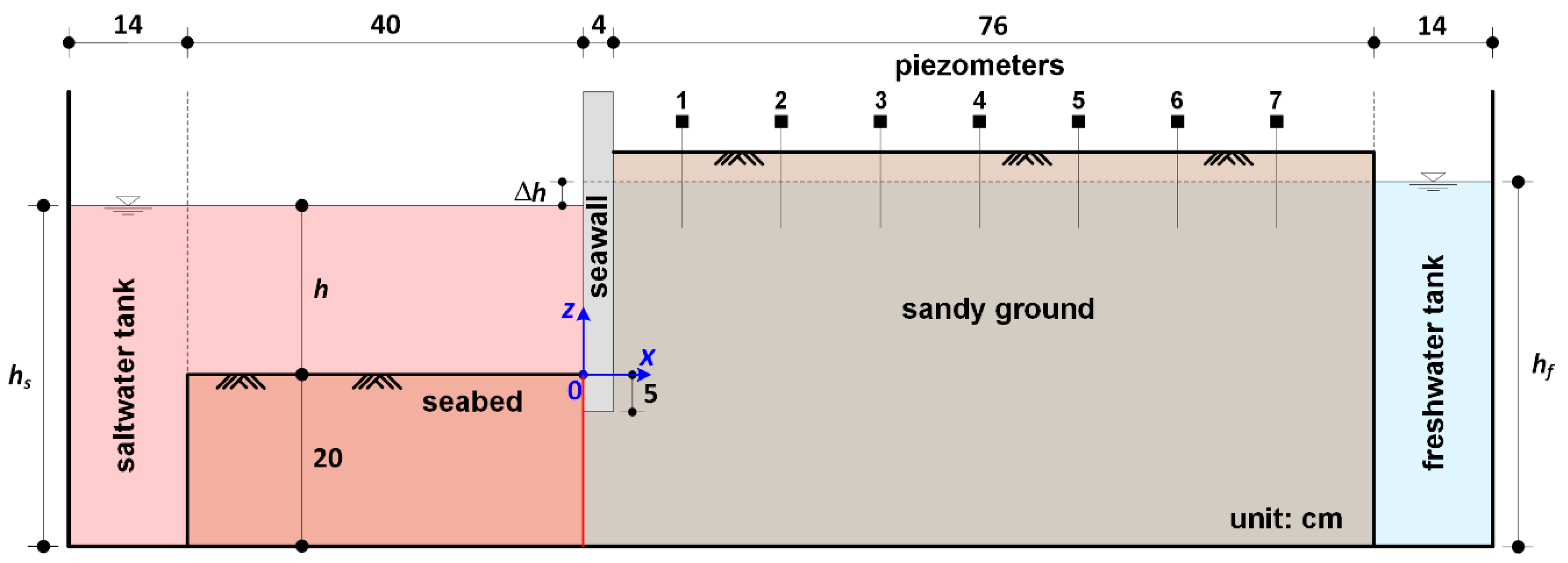
The sandy tank shown in
Figure 1 was constructed to investigate the formation process of the saltwater-freshwater interface in the coastal aquifer with a seawall [
19]. The dimensions of the sandy tank are as follows: 148 cm length, 50 cm height, and 20 cm width. On both sides of the sandy tank, compartments of 14 cm length and 20 cm width were constructed to maintain constant water level and salinity of the saltwater and freshwater. In these compartments, separate saltwater/freshwater injection tanks and flow control devices were connected to maintain the target water level and salinity. The compartment walls consisted of dense stainless steel wire meshes, which allowed water to pass through freely but blocked sand. The experimental tank was divided into sea and land regions with lengths of 40 cm and 80 cm, respectively, by constructing an impermeable upright seawall with a thickness of 4 cm. The thickness of the seabed in the sea region was 20 cm, and the ground behind the seawall was laid higher with sand than the groundwater level.
2.2. Experimental Conditions and Measurements
To track the saltwater–freshwater interface in the coastal aquifer, the saltwater was stained with a Rhodamine B reagent. The water used in the experiment was normal clean tap water, and purified salt was dissolved in the saltwater to reach the target salinity. The salinity, water temperature, and density in each experiment were measured and adjusted to maintain constant experimental conditions. The sand forming the seabed and coastal aquifer was standard filter sand with a particle diameter of 0.8–1.2 mm, an average particle diameter of 1 mm, and a porosity of 0.41.
The experimental conditions were largely based on differences between the sea level and groundwater level (Δh) and between the saltwater and freshwater salinities (ΔS). At a sea depth (h) of 20 cm, Δh was set to 1 cm, 1.5 cm, and 2 cm, and at h = 10 cm, Δh was set to 1 cm and 1.5 cm. In addition, as the freshwater salinity was 0 psu, and ΔS was 25 psu, 35 psu, and 45 psu. In each experiment, saltwater and freshwater were injected into the compartments of the sandy tank to stably reach the target water level as quickly as possible.
Seven piezometers were arranged at intervals of 10 cm to measure the groundwater level behind the seawall. The detailed locations are shown in
Figure 1. Additionally, the saltwater–freshwater interface in the coastal aquifer was extracted from the digital images by an image processing technique based on a two-dimensional analysis of the RGB pixels.
2.3. Experimental Results
The experimental results were measured when the groundwater flow in the coastal aquifer reached a steady state or when the saltwater-freshwater interface reached equilibrium. Although the time to reach a steady state varies depending on the experimental conditions, it represents the time when changes in the groundwater level of the coastal aquifer and the saltwater-freshwater interface rarely occur for an extended period. In the experimental condition used in this study, the steady state was reached after approximately 30 min to 1 h.
2.3.1. Groundwater Table
Figure 2 shows the distribution of groundwater level behind the seawall in typical laboratory experiments and numerical simulations. Only the experimental results are discussed in this section. A comparison with the numerical results is provided later with the validation of the numerical model.
In
Figure 2, the difference between the sea level and groundwater level decreases towards the sea. However, the difference between the sea level and that behind the seawall is maintained to some extent due to the groundwater blocking effect of the seawall. The larger the value of Δ
h, the more pronounced the effect, and the greater the water level difference in front of and behind the seawall. As a result, the larger the water level difference between the coastal aquifer and the sea, the more groundwater flow develops and the higher the pressure gradient. This distribution of groundwater level in the coastal aquifer has a large influence on the formation of the saltwater–freshwater interface.
2.3.2. Pressure-Equilibrium State
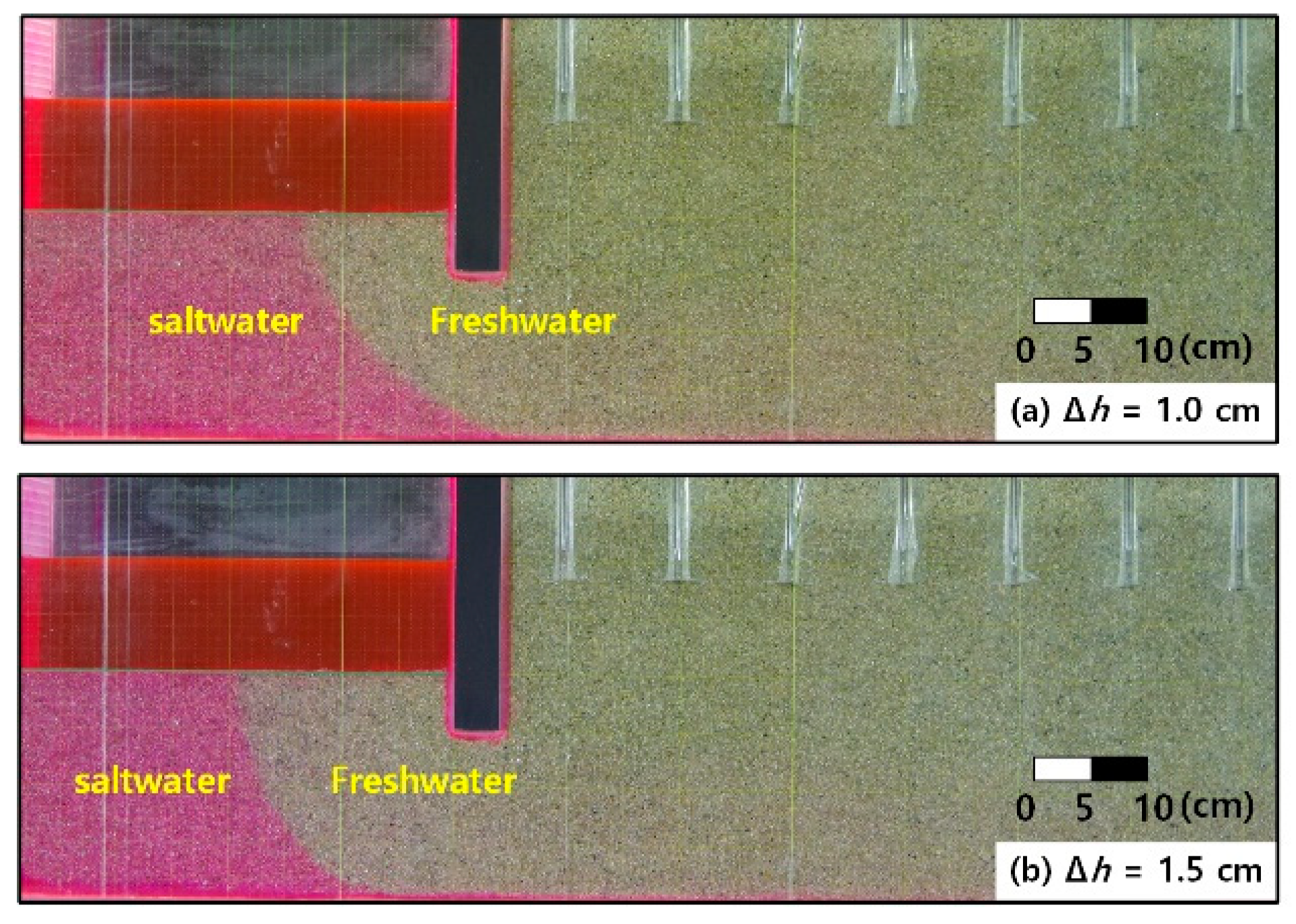
Figure 3 shows an image taken when the saltwater and freshwater were parallel at
h = 10 cm. Here, the red section is the saltwater region stained with a reagent, and the remainder is the freshwater region.
In
Figure 3, the larger the value of Δ
h, the more the saltwater–freshwater interface is distributed towards the seabed. This is because as Δ
h increases, the pressure gradient increases and the groundwater flow of the coastal aquifer becomes stronger, causing the saltwater–freshwater interface to be pushed outwards. Furthermore, a region develops in the seabed in front of the seawall, through which groundwater (freshwater) escapes but saltwater cannot intrude. This is a unique saltwater–freshwater interface that was not observed in previous studies, which did not consider underground obstructions.
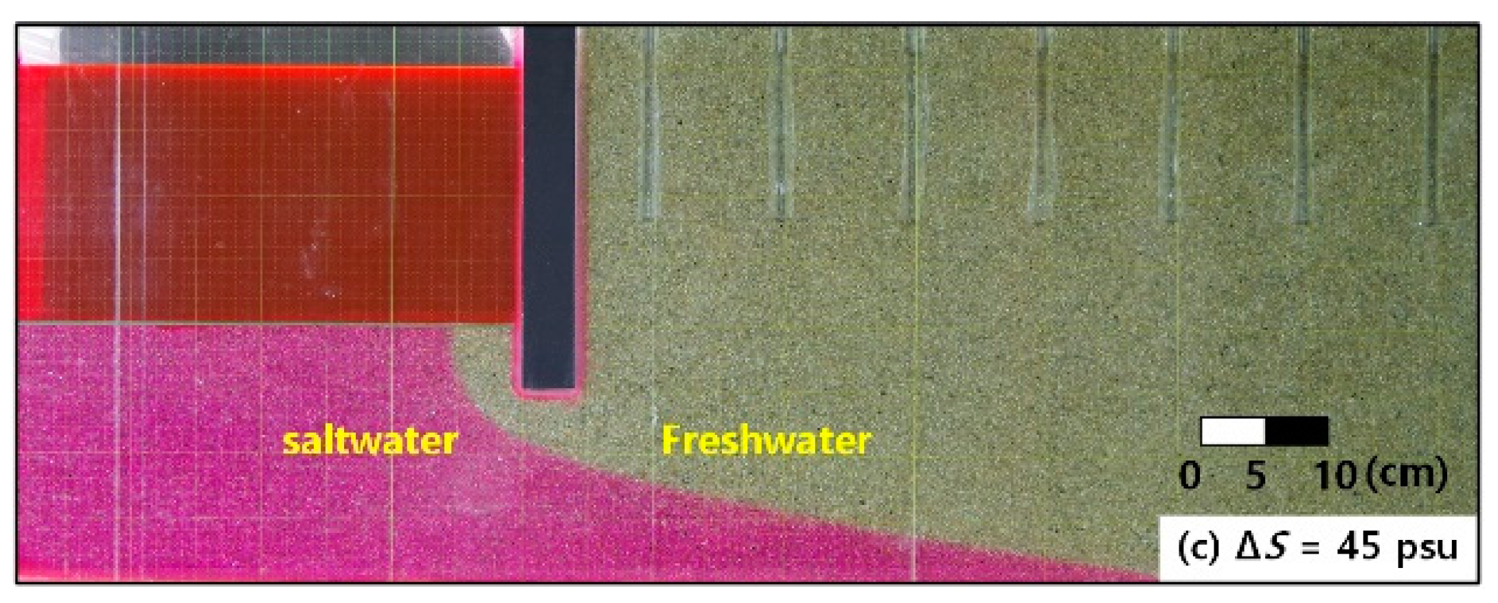
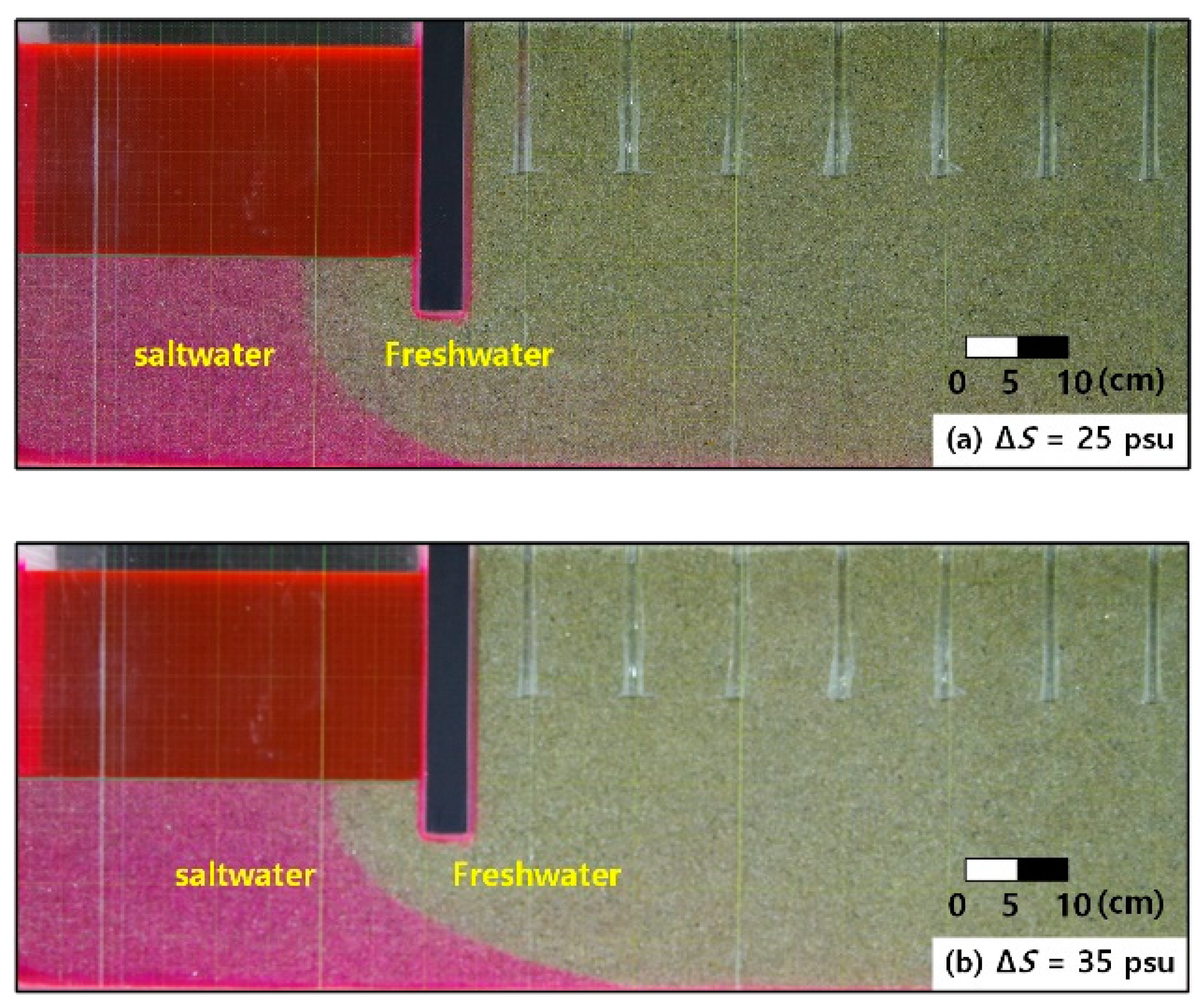
Figure 4 shows the parallel state of saltwater and freshwater at typical conditions according to Δ
S.
In
Figure 4, the larger Δ
S, the larger the reduced gravity (
g’ = Δ
ρg/
ρf; Δ
ρ is the difference in the density of saltwater and freshwater,
g is gravitational acceleration, and
ρf is the freshwater density), facilitating saltwater intrusion into the coastal aquifer. Thus, at the same Δ
h, the higher the salinity, the gentler the pressure gradient of the coastal aquifer and the stronger the flow rate of the saltwater intrusion, resulting in the deep intrusion of the saltwater–freshwater interface into the coastal aquifer. As mentioned above, the groundwater escapes through the freshwater region through the seabed in front of the seawall; the unique saltwater–freshwater interface distribution caused by the pressure equilibrium can be re-confirmed.
2.3.3. Saltwater–Freshwater Interface
While the saltwater–freshwater equilibrium interface has been discussed in Lee et al. [
19], their experimental results exceeded the measurement limits of the sandy tank. Therefore, this study reanalyses the characteristics of the saltwater–freshwater equilibrium interface with only measurement results within the allowable range.
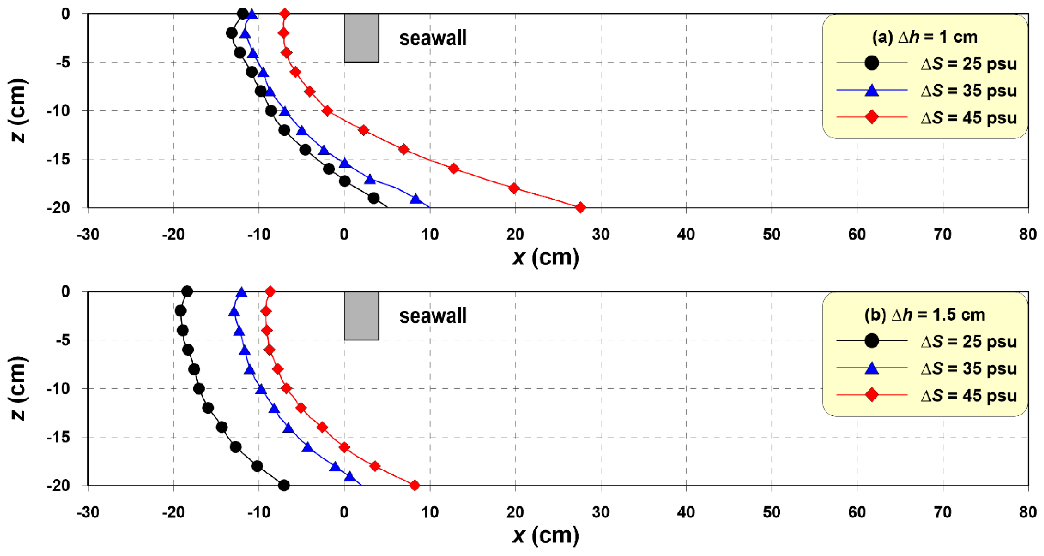
Figure 5 compares the saltwater–freshwater equilibrium interfaces according to Δ
S.
In
Figure 5, when Δ
h is constant, the larger the Δ
S, the gentler the pressure gradient of the coastal aquifer and the larger the reduced gravity, causing more saltwater to intrude into the aquifer. Comparing
Figure 5a,b, the pressure gradient of the coastal aquifer increases with Δ
h; as a result, the saltwater–freshwater equilibrium interface tends towards the sea side, and the interface slope becomes steep. This is because as Δ
h increases, the flow rate of the groundwater increases, pushing the saltwater–freshwater interface towards the sea.
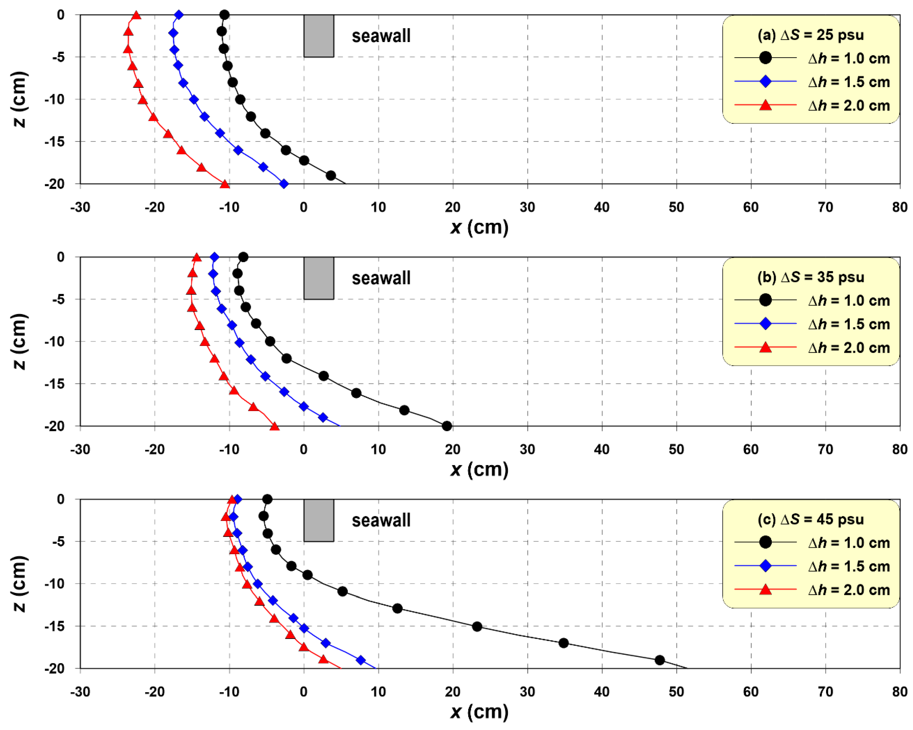
Figure 6 compares the saltwater–freshwater equilibrium interface with respect to Δ
h for each Δ
S at a sea depth of 20 cm.
In all graphs of
Figure 6, the pressure gradient of the coastal aquifer increases with Δ
h, causing the distribution of the saltwater–freshwater interface to tend towards the sea side. Comparing (a), (b), and (c), the smaller Δ
S, the smaller the pressure gradient and reduced gravity, weakening saltwater intrusion in the coastal aquifer.
The above results indicate that saltwater intrusion in the coastal aquifer strengthens as the pressure gradient decreases (smaller Δh, larger ΔS). Conversely, as the pressure gradient increases (larger Δh, smaller ΔS), the saltwater–freshwater interface is distributed on the sea side, and saltwater intrusion does not occur even behind the seawall. In addition, because groundwater escapes beneath the seawall, unique saltwater–freshwater interface and freshwater region are formed, in which saltwater cannot intrude.
On a related note, we discuss the groundwater hydraulic characteristics of the seawall-constructed coastal aquifer in depth through a numerical analysis, considering that these characteristics are difficult to sufficiently understand through the sandy tank experiment.
3. Numerical Analysis
Groundwater flow is mainly affected by aquifer characteristics of heterogeneity, discontinuity, and anisotropy [
20,
21,
22]. However, most numerical models simulating seawater intrusion in coastal aquifers interpret groundwater flow as dependent on hydraulic conductivity. Therefore, this study introduces a numerical model—Navier-Stokes equation model based on PBM—that can account for the characteristics of the aquifer more precisely. This model can be used to analyse flow considering the energy dissipation of the groundwater according to particle diameter, porosity, and shape of the aquifer, as well as directly simulate changes in flow due to impermeable obstructions.
3.1. Numerical Model
3.1.1. Governing Equations
The basic set of calculations consists of the continuity equation (Equation (1)), which includes the source term that generates flows without disturbance in 3D incompressible and viscous fluids, and a modified Navier-Stokes momentum equation (Equation (2)), in which the fluid resistance of the porous media is applied.
where
is the Cartesian coordinate system (
,
and
); the
-axis is a vertical axis with zero indicating seabed-face and positive values upward;
is the velocity component corresponding to the
direction;
is the volume porosity;
is the surface porosity in the
direction;
is the flux density of the source and sink term;
is time;
is the fluid density;
is the fluid pressure;
is the sum of the kinematic viscosity coefficient (
) and the eddy viscosity coefficient (
) from the turbulence model;
is the strain rate tensor;
is the surface tension force based on the continuum surface force model [
23];
is the source and sink terms;
is the fluid resistance term for the porous media;
is the acceleration of gravity term; and
is the wave energy damping term for the added damping zones.
A numerical simulation of fluid flow with a free surface requires not only solutions of governing equations (Equations (1) and (2)) but also special treatment of the free surface (i.e., tracking of the fluid interface). In this study, the free surface is governed by Equation (3) in terms of the volume of fluid (VOF) function [
24] based on incompressibility fluid and PBM, which represents the rate of fluid volume in the cell to the entire cell volume.
where
is the VOF function.
3.1.2. Fluid Resistances in Porous Media
The fluid resistance for flow through porous media,
in Equation (2) applied in this study is shown in Equation (4). The fluid resistances include the frictional resistance forces due to laminar flow (viscous effect) by Liu and Masliyah [
25], the frictional resistance forces due to turbulent flow (turbulence effect) by Ergun [
26], and the inertia resistance force suggested by Sakakiyama and Kajima [
27].
where
is the coefficient of laminar resistance;
is the coefficient of turbulent resistance;
is the coefficient of inertia; and
is the median grain size of porous media.
3.1.3. Equations of State for Fluids
To analyse density current, it is important to estimate the density of a fluid accurately; thus, Equation (5) was applied to estimate density according to temperature and salinity, as suggested by Gill [
28].
where,
ρ0 is the density of 4 °C fresh water.
is the increase in density with temperature change and is expressed as Equation (6).
expresses the change in density with changing salinity and is expressed as Equation (7). The empirical constants used in the density calculation are shown in
Table 1.
where
is the temperature (°C), and
is the salinity (psu).
The kinematic viscosity coefficient
for the fluid is calculated using Equation (8). Here, the calculated value of Equation (5) is substituted for density
, and the viscosity coefficient
is calculated using Equation (9), which considers water temperature and salinity, as suggested by Riley and Skirrow [
29].
where,
is the viscosity coefficient for 4 °C freshwater.
indicates the change in the viscosity coefficient with a change in temperature and is expressed as Equation (10).
indicates the change in the viscosity coefficient with a change in salinity and is expressed as Equation (11). The empirical constants used for the water viscosity coefficient are expressed in
Table 2.
3.1.4. Advection-Diffusion Equations
In density current analyses, quantitative decisions about influential factors are important in order to accurately calculate the fluid density
and kinematic viscosity coefficient
, which are substituted into the governing equations. The state equation used to calculate the density and kinematic viscosity coefficient of water is a function of temperature
and salinity
. Therefore, the advection-diffusion equations adopted herein include Equation (12) for temperature and salinity.
where
is
or
;
is the diffusion coefficient;
is the eddy viscosity coefficient simulated by the turbulence model; and
is the Prandtl/Schmidt number.
3.1.5. Solution Techniques
A staggered grid is used for computational discretization, where the velocity components are stored at the cell face, and other variables including the pressure, wave source function, and VOF function are defined at the cell centre. The governing equations are converted to a system of algebraic equations using the finite difference method. For the discretization of the Navier-Stokes momentum equation (Equation (2)), we use the forward difference approximation for time derivative terms, a combination of the central difference and upwind methods for the convection term, and the central difference approximation for the other terms, including the pressure gradient and stress. The finite difference approximations of Equation (2) can be written as:
From the discretized Equation (14), new water particle velocities can be calculated explicitly using initial conditions or velocities and the pressure in the satisfaction of divergence at the previous time step. However, the flow velocity calculated using only the momentum equation (Equation (14)) cannot satisfy the continuity equation in a control volume. Therefore, this study uses the numerical SOLution Algorithm (SOLA) for transient fluid flow scheme, sometimes called the highly simplified maker and cell (HSMAC) technique, which performs iterations for flow velocities to satisfy the continuity equation (Equation (1)) while also properly adjusting the pressure.
D < 0 in (15) means that the mass flows into the cell. Therefore, the pressure (
) must be increased to prevent this. By contrast,
must be decreased for
. Because
exists in a cell,
can be adjusted properly to induce
to reach divergence (
), and it can be defined as follows regarding
as a function of
. Therefore, to solve
, the Newton-Raphson method can be applied as Equation (16).
where
has influence on the neighbouring cell (meaning that repeated calculations are required), and the superscript
represents the number of iterations at each time step. The calculation is repeated until the designated convergence condition is satisfied, and the updated pressure and flow velocity at each cell based on the repetitions are then expressed as the following Equations (17) and (18), respectively.
The iterations continue until all divergences are made sufficiently small such that the velocity field is within the accuracy requirements. In this study, the magnitude of is chosen to be approximately times a typical absolute value of . The last iterated quantities of velocity and pressure are taken as the advanced time values.
After velocity components and the pressure have been calculated, the new free surface configuration is computed using the advection equation of the VOF function (Equation (3)), which is solved by using the donor-acceptor method [
24].
3.1.6. Boundary Conditions and Stability
Two free surface boundary conditions (i.e., normal and tangential stress conditions) are used to conduct the time-marching scheme of free surface motion. The normal stress condition is imposed as a boundary condition for pressure. The pressure point defined in the centre of a cell generally differs from the actual location on the free surface. Therefore, the pressure in the centre of the surface cell is evaluated using linear interpolation or extrapolation between the pressure on the free surface and that of the adjacent fluid cell. The tangential boundary condition is imposed by assuming the same velocities outside the fluid domain as those in the fluid domain (zero gradient boundary condition on the free surface). Furthermore, the velocities on the interfaces between the surface and empty cells are determined in such a manner as to satisfy the continuity equation.
The impermeable and non-slip conditions are applied on the normal and tangential directions to the bottom and surface of the structure, respectively. The slip condition is also imposed as a lateral boundary condition for the
x-z plane when taking
y = 0 and the outermost opposite
x-z plane. From this lateral condition, it can be assumed that the infinite width in the
y-direction is considered under the condition that the direction of the flow wave is perpendicular to the seawall, and thus the dimension of the numerical water tank can be reduced for efficient calculation. In addition, at both ends of the numerical water tank, the radiation condition (open boundary), in which the change in physical quantity (
), such as velocity or VOF function, becomes 0, is added as follows:
In computational fluid dynamics, the stability of calculation, which is related to the convergence of the numerical solution, is critical. In this study, the Courant–Friedrichs–Lewy (Equation (20)) and the diffusive limit condition (Equation (21)) are imposed to determine the time interval
.
where
is the maximum velocity corresponding to the
direction and
is the weighting coefficient, which was chosen as
in most cases.
s under laboratory conditions and
s under normal field conditions are used for the initial time intervals, after which the time interval
is adjusted automatically each hour to satisfy the Courant condition (Equation (20)) and the diffusive limit condition (Equation (21)).
3.2. Validation of Numerical Model
To verify the validity and effectiveness of the numerical model, a numerical sandy tank is constructed on the basis of the sandy tank experiment, as shown in
Figure 1. The specifications and calculation conditions of the numerical tank are the same as in the experiment. In both compartments of the numerical tank, a source and a sink were arranged to keep the water level and salinity constant. To verify the numerical model, the numerical sandy tank was divided by intervals of 0.2 cm horizontally and vertically to form a square grid, and calculations at intervals of 1/20 s were conducted.
As shown in
Figure 2, the calculated values, groundwater level, and surface slope of the area behind the seawall show high agreement between the sandy tank experiment and numerical simulation, and the groundwater level difference is also accurately reproduced. This is because the numerical model accurately reproduces the flow generation and fluid resistance of the sandy ground by the water level difference.
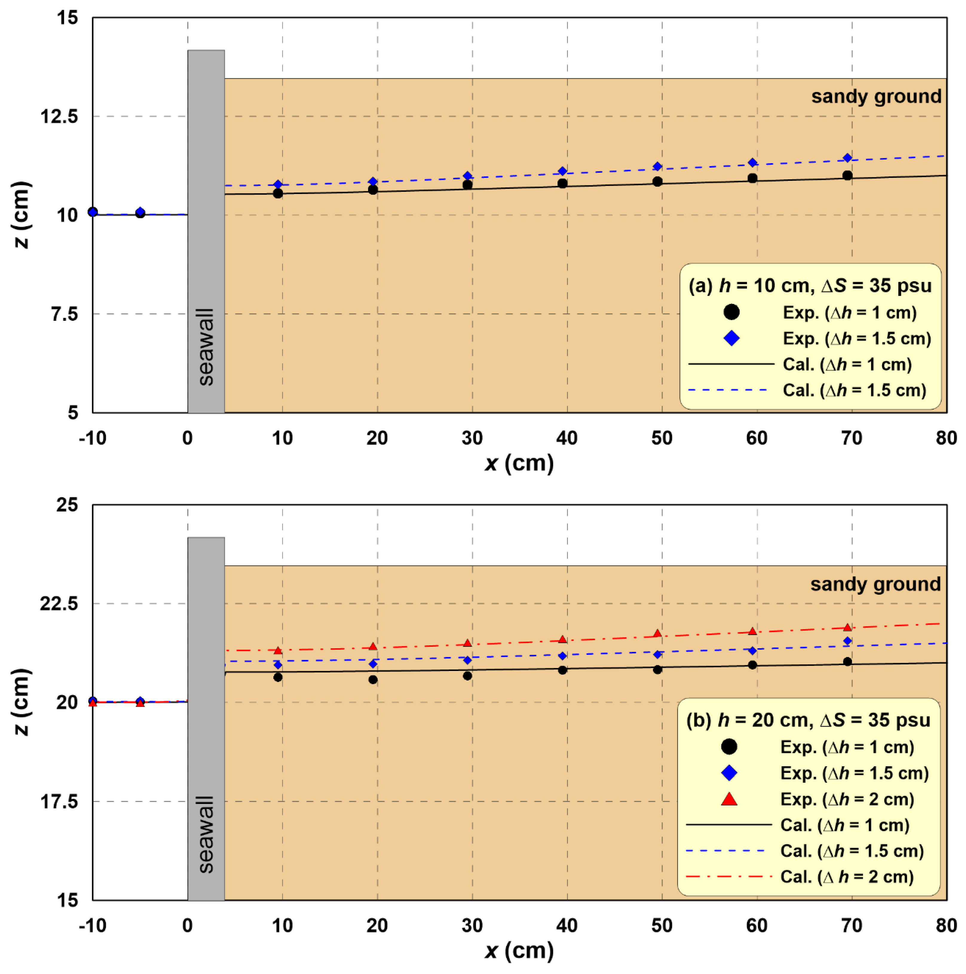
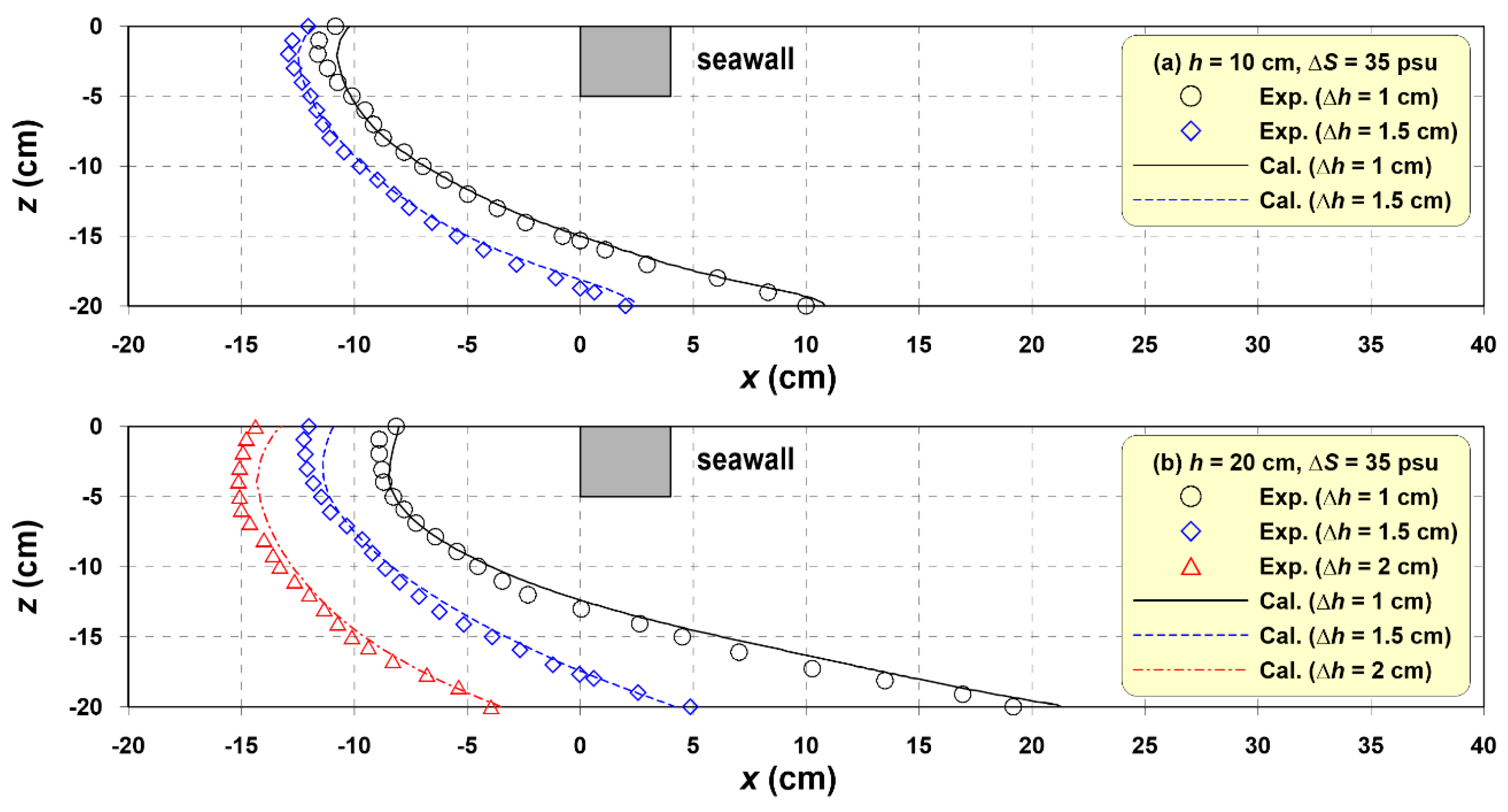
Figure 7 shows the saltwater–freshwater equilibrium interface for (a)
h = 10 cm and (b)
h = 20 cm with Δ
h at Δ
S = 35 psu. Here, the saltwater–freshwater interface is defined as an isohaline of 17.5 psu, which is half the salinity.
In
Figure 7, while the saltwater–freshwater interface in the numerical computation slightly overestimates saltwater intrusion, it reproduces the saltwater–freshwater interface measured in the experiment with sufficient accuracy. In particular, the calculation results accurately show the characteristics of the unique saltwater–freshwater interface attributable to the effect of the seawall.
To confirm the statistical accuracy of the numerical model, the normalized root mean square error (NRMSE) was calculated using Equation (22). In the calculation of RMSE and NRMSE, the groundwater level was calculated based on seven measurement values in the experimental sandy tank, and for the saltwater-freshwater interface, 20 interface horizontal distances at each of the vertical positions at 1 cm intervals were used.
where
is the amount of data,
is the measured value, and
is the calculated value.
In addition to the qualitative reproducibility of the numerical models shown in
Figure 2 and
Figure 7, the statistical accuracies are listed in
Table 3. Under laboratory-scale conditions, the average NRMSE of the groundwater level in the coastal aquifer was 0.093, and the NRMSE of the saltwater-freshwater interface was 0.076, which verified the validity of the numerical analysis.
3.3. Numerical Conditions
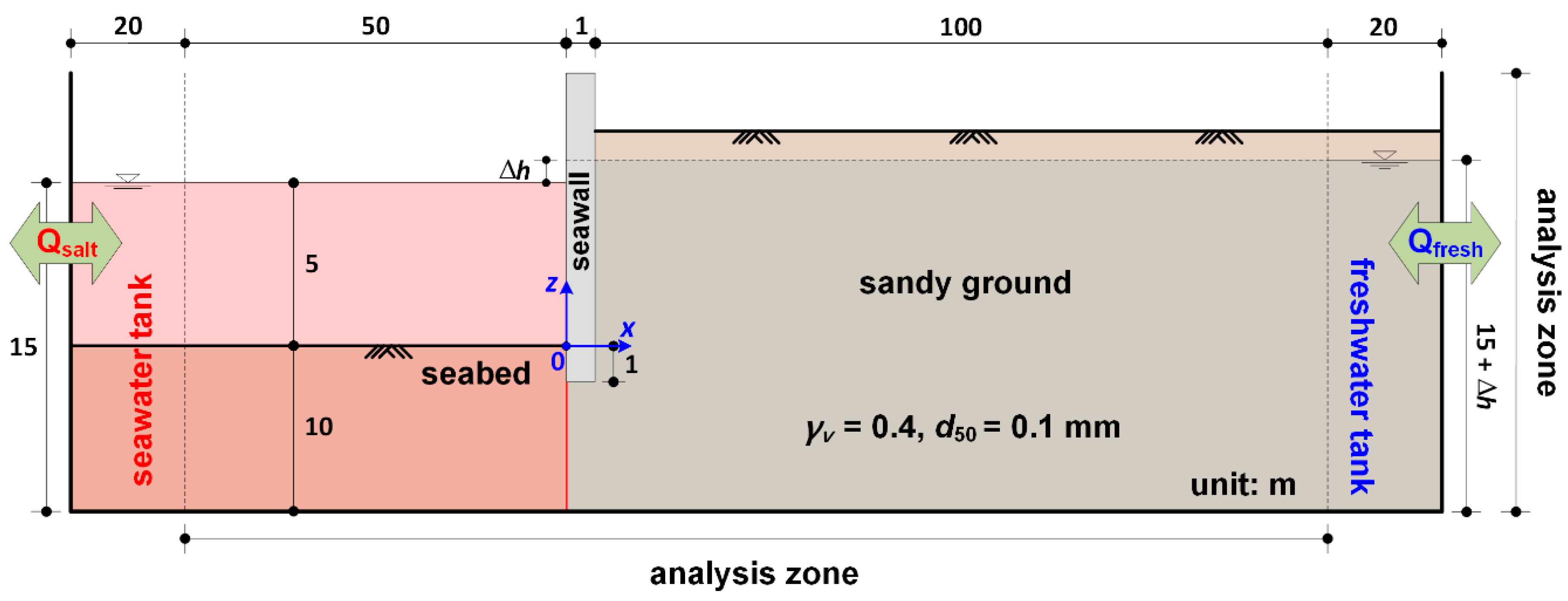
Through close numerical analysis, we investigate the groundwater flow in the coastal aquifer, pore water pressure distribution, and the formation process of the seawater–freshwater equilibrium interface under the practical condition for scale, which could not be verified in the scale model experiment. To this end, a numerical sandy tank was constructed, as shown in
Figure 8. The analysis area of the numerical water tank is 151 m × 20 m, and compartments are arranged on both sides to maintain the constant water level and salinity of the seawater and groundwater. The sea depth (
h) is 5 m, seabed thickness (
D) is 10 m, porosity (
γv) of the seabed and the coastal aquifer is 0.4, and mean particle diameter (
d50) is 0.1 mm. The calculation area was divided by intervals of 0.25 m horizontally and vertically to form a square grid, and calculations were conducted at intervals of 1 s. Regarding the numerical analysis conditions, the salinity of the seawater is 30 psu, and the temperature difference between the seawater and groundwater is not considered. The difference between the sea level and groundwater level is shown in
Table 4. At both boundaries of the water tank, a source and a sink were arranged to maintain the constant water level and salinity.
3.4. Numerical Results
The present study discusses numerical results for the steady state, which showed that very little change occurred in the groundwater flow and water levels in the coastal aquifer. In addition, the seawater-freshwater interface was observed over time. The time to reach the steady state was different depending on the numerical calculation conditions, and under the numerical condition used in this study, the steady state was reached in approximately 24–36 h.
3.4.1. Groundwater Table
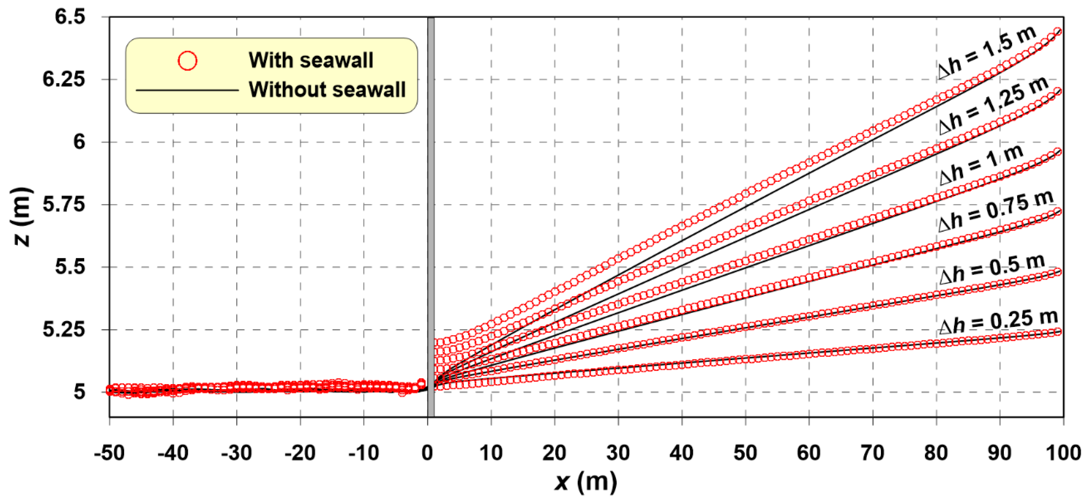
To examine the effects of the construction of an artificial seawall on the groundwater level distribution of the coastal aquifer, we compare the groundwater level distribution according to the construction of the seawall (
Figure 9). Here, the solid lines and circles indicate the water level with and without the construction of the seawall, respectively.
As shown in
Figure 9, the groundwater level gradually decreases at a constant slope and equals the sea level near the shoreline (
x = 0 m). However, the water level behind the seawall rises because of the groundwater blocking effect of the seawall. As discussed in the sandy tank experiment, the larger Δ
h, the more pronounced the water level difference in front of and behind the seawall. The water level distribution in the coastal aquifer is closely related to the groundwater flow, pore water pressure, and formation of the seawater–freshwater interface. These are discussed in depth later in the paper.
3.4.2. Groundwater Flow
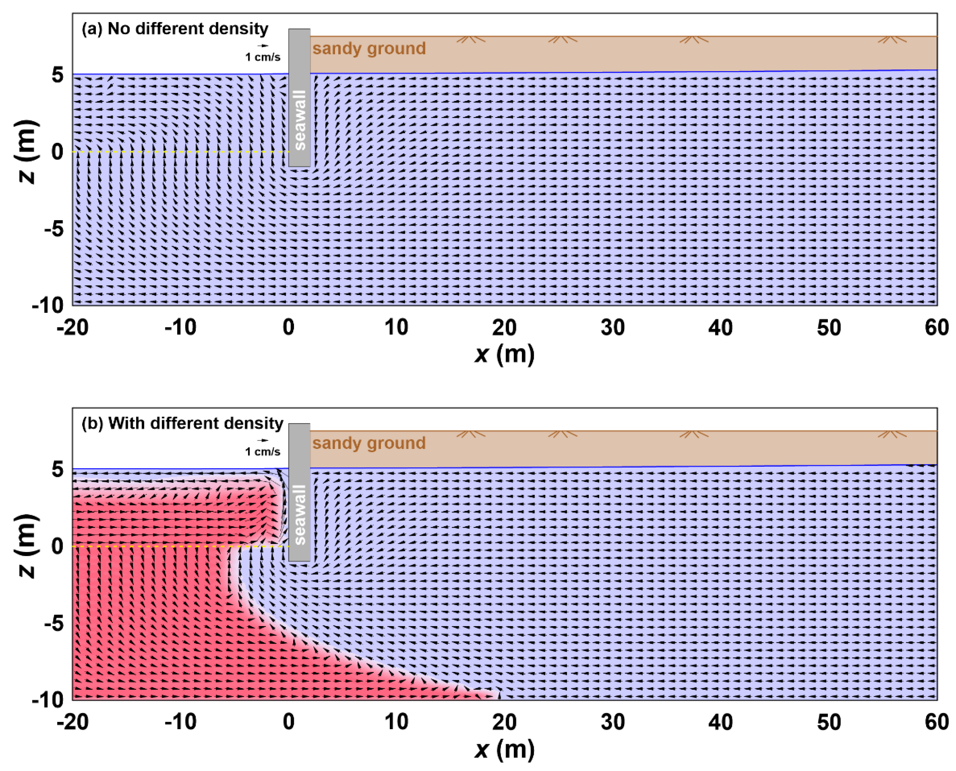
To confirm the groundwater flow characteristics in the coastal aquifer with a seawall,
Figure 10 compares the cases of no difference in density and different densities between the seawater and groundwater.
In
Figure 10a, the groundwater flow below the seawall is widely distributed overall, and the flow rate is not very large. Conversely, in
Figure 10b and the coastal aquifer with both saltwater and freshwater, dense seawater (saltwater) intrudes below the groundwater (freshwater) in a wedge shape. As a result, the movement path of the groundwater that escapes to the sea due to the water level difference becomes considerably narrow, and the flow rate increases. Therefore, a freshwater region is formed in the seabed in front of the seawall through which the groundwater escapes, as confirmed in the sandy tank experiment.
In contrast, as shown in
Figure 10, the flow pattern completely differs depending on whether the density difference between the seawater and groundwater is considered. Accordingly, to understand the hydraulic characteristics of the groundwater in the coastal aquifer, it is necessary to numerically analyse the difference in the density of the seawater and groundwater, as performed in this study.
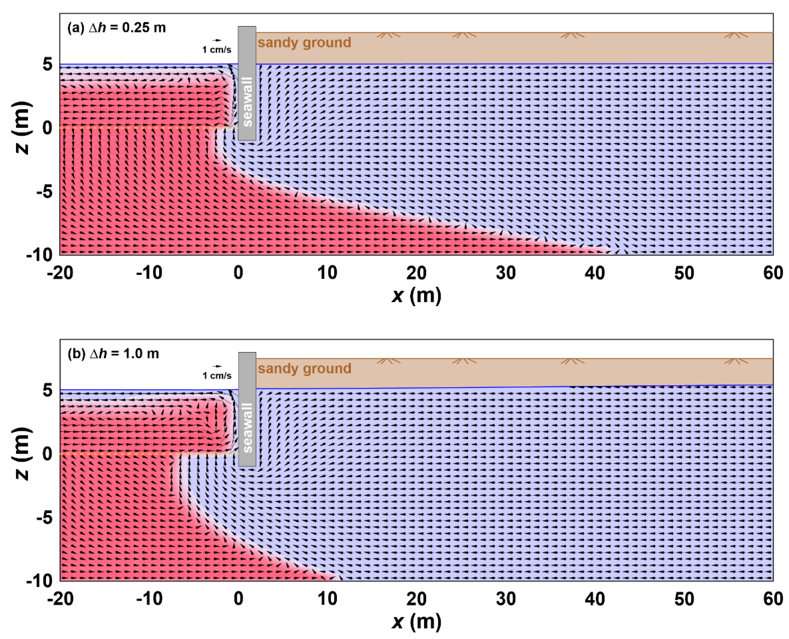
Figure 11 shows a comparison and analysis of the distribution characteristics of the groundwater flow and seawater–freshwater equilibrium interface according to Δ
h.
As confirmed in
Figure 11, dense seawater exists in the shape of a wedge below the groundwater. In addition, the water level difference between the front and back of the seawall shown in
Figure 10 is small.
Figure 11a, in which the groundwater level slope is gentle, shows deeper seawater intrusion inland than
Figure 11b. In addition, when the water level difference is small, the pressure gradient and flow rate of the groundwater are small; as a result, the force pushing the seawater towards the sea is insufficient, and a freshwater region narrowly forms on the seabed in front of the seawall.
As described above, while the groundwater level, groundwater flow, and the distribution of the seawater–freshwater interface of the coastal aquifer with a seawall were examined in the sandy tank experiment, this analysis provided an understanding of the formation mechanism of the freshwater region of the seabed in front of the seawall and the unique seawater–freshwater interface.
3.4.3. Pore Water Pressure
In the sandy tank experiment and the numerical analysis described above, we discussed the relationship between the pressure gradient and the seawater–freshwater interface of the coastal aquifer according to Δ
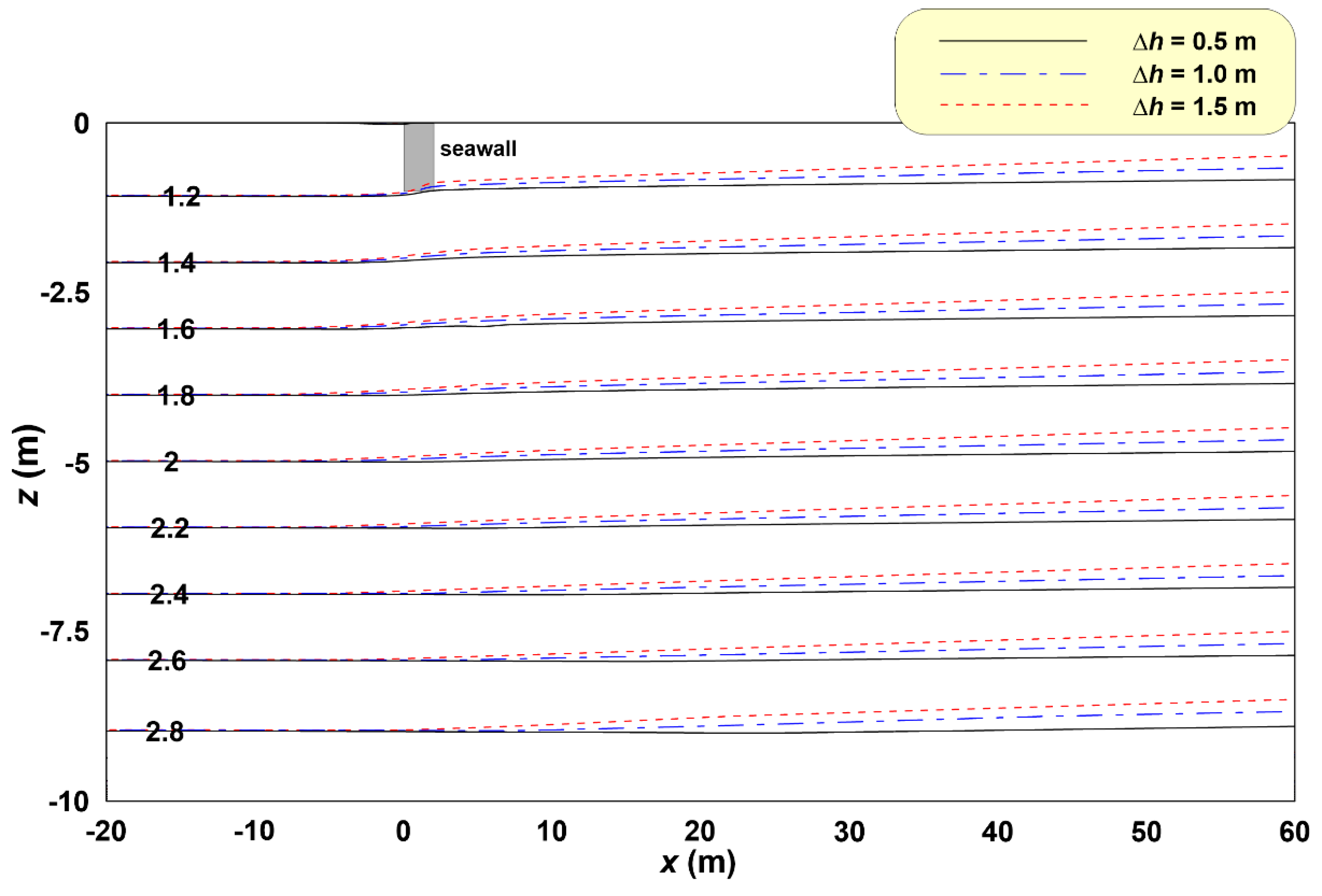
h. To clearly understand this correlation, we analysed the pore water pressure of the coastal aquifer through the numerical analysis, which could not be examined using the existing numerical models. Pore water pressure was directly calculated using the Navier-Stokes solver, a PBM-based non-hydrostatic model. In
Figure 12, the pressure gradients are compared and analysed by plotting contour lines for typical conditions of Δ
h = 0.5 m, Δ
h = 1 m, and Δ
h = 1.5 m. Here, the pore water pressure was divided by the hydrostatic pressure (
ρsgh;
ρs is the seawater density,
g is the gravitational acceleration, and
h is the sea depth) at a seabed depth of 5 m.
As already observed in
Figure 12, the greater Δ
h, the greater the pore water pressure gradient in the coastal aquifer. In particular, the slope of the non-dimensional contour line 1.2 formed under the seawall, in which the largest water level difference suddenly occurs.
Here, we qualitatively examined the effect of the pressure gradient on the distribution of the seawater–freshwater equilibrium interface. In the coastal aquifer, a seawater–freshwater interface forms in the region in which an equilibrium of the seawater fluid force is reached due to the fluid force and gravity of the groundwater due to the pressure gradient. This distribution of pore water pressure in the coastal aquifer plays a key role in forming the seawater-freshwater equilibrium interface. A more in-depth analysis is required to understand this close correlation. Accordingly, a quantitative analysis of this phenomenon will be conducted in the future.
3.4.4. Seawater–Freshwater Interface
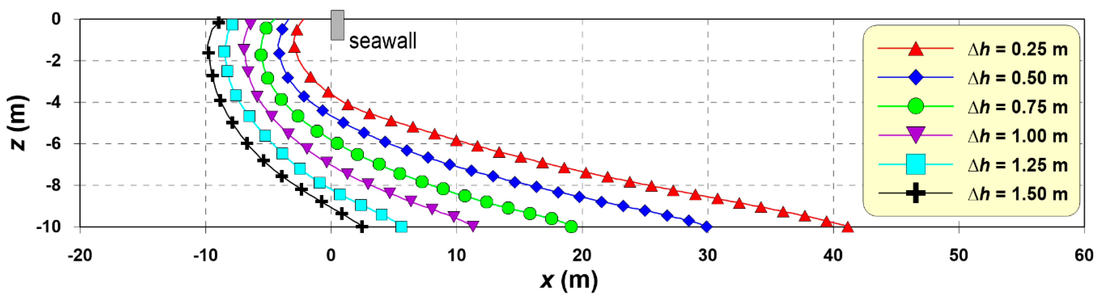
Figure 13 shows the seawater-freshwater equilibrium interface measured at each Δ
h condition in the numerical sandy tank. The seawater–freshwater interface was defined as an isohaline of 15 psu, which is half of the seawater salinity.
Comparing the seawater–freshwater interface according to Δ
h in
Figure 13, the larger Δ
h, the more the equilibrium interface tends towards the sea side. In addition, a freshwater region widely forms on the seabed in front of the seawall. This phenomenon is consistent with the results already confirmed in the sandy tank experiment, and the results of the water level, flow, and pore water pressure distribution in the coastal aquifer are also consistent. In addition, as measured in the sandy tank experiment, seawater intrusion in the coastal aquifer barely occurs if the difference between the sea level and groundwater level is large.
According to the experimental and numerical analysis results, the pressure gradient and groundwater flow rate increase as Δh increases in the aquifer with a seawall. As a result, the seawater–freshwater interface is pushed towards the sea and a freshwater region forms on the seabed in front of the seawall through which the groundwater escapes. Accordingly, this study allows us to understand the formation mechanism of the seawater–freshwater interface in a coastal aquifer with an underground obstruction such as a seawall.
4. Conclusions
In this study, sandy tank experiment and numerical analysis were conducted to investigate the effect of underground obstructions, such as a seawall, on the hydraulic characteristics of the groundwater in a coastal aquifer. In the experiment, the saltwater–freshwater equilibrium interface was measured in a sandy tank in which an impermeable upright seawall was constructed. In the numerical analysis, a non-hydrostatic numerical model, which can directly analyse the groundwater flow according to the characteristics (particle diameter, porosity, shape, etc.) of the porous medium, was introduced. This is a departure from conventional methods that depend on hydraulic conductivity. In the numerical sandy tank with a seawall, we analysed the groundwater flow, water level, and pore water pressure distribution within the coastal aquifer. These analyses revealed the formation mechanism of the seawater–freshwater equilibrium interface. The main results obtained from the sandy tank experiment and numerical analysis are as follows.
- (1)
As Δh increases, the water level difference between the front and back of the seawall measured in the sandy tank increases, and the distribution of the saltwater–freshwater interface tends towards the sea side.
- (2)
As ΔS increases, the reduced gravity increases, thereby facilitating saltwater intrusion into the coastal aquifer. As a result, at the same Δh, as ΔS increases, the saltwater–freshwater interface becomes more widely distributed in the coastal aquifer.
- (3)
The PBM-based Navier-Stokes solver was introduced to simulate seawater intrusion in the coastal aquifer; PBM can directly consider the characteristics (particle diameter, porosity, shape) of the permeable medium.
- (4)
The accurate reproduction of the groundwater level and saltwater–freshwater interface of the coastal aquifer measured in the sandy tank demonstrated the validity and effectiveness of the Navier-Stokes solver introduced in this study.
- (5)
Due to the groundwater blocking effect of the seawall, the difference between the water level behind the seawall and the sea level increased, and this tendency became more pronounced with increasing Δh.
- (6)
In the seawall-constructed coastal aquifer, the groundwater flow rate increased as Δh increased, and the unique groundwater flow and seawater–freshwater interface were formed in the numerical analysis when the difference in density between the seawater and freshwater was considered.
- (7)
In the sandy tank experiment and numerical analysis, there were also cases in which seawater intrusion in the coastal aquifer did not occur due to the rise in groundwater level caused by the groundwater blocking effect of the seawall.
- (8)
In the non-hydrostatic numerical model, for the pore water pressure of the coastal aquifer, the pressure gradient increased as Δh increased. In addition, due to the large difference in water level in front of and behind the seawall, the largest pressure gradient occurred directly underneath the seawall.
- (9)
The numerical analysis also showed a unique distribution of the seawater–freshwater interface near the seawall, similar to that in the sandy tank experiment. Moreover, from the overall hydraulic characteristics of groundwater flow, water level, and pore water pressure of the coastal aquifer obtained through the numerical analysis, the formation process of the seawater–freshwater interface could be understood.
- (10)
This formation of the seawater–freshwater interface in the seawall-constructed coastal aquifer occurred due to the groundwater flow and pressure gradient caused by the difference in water level. As Δh increased, the seawater–freshwater interface tended towards the sea side, and a freshwater region was widely formed in the seabed in front of the seawall through which groundwater escaped.
Based on the experimental and numerical analysis results, groundwater is partially blocked by underground obstructions such as seawalls, thereby inducing a rise in the water level. As a result, the pressure gradient and groundwater flow rate of the coastal aquifer increase, slowing seawater intrusion. Therefore, this principle can be applied to seawater intrusion reduction in coastal aquifers to more actively respond to seawater intrusion due to rises in the sea level and decreases in groundwater level.


