Numerical Simulation of Non-Homogeneous Viscous Debris-Flows Based on the Smoothed Particle Hydrodynamics (SPH) Method

Abstract

Non-homogeneous viscous debris flows are characterized by high density, impact force and destructiveness, and the complexity of the materials they are made of. This has always made these flows challenging to simulate numerically, and to reproduce experimentally debris flow processes. In this study, the formation-movement process of non-homogeneous debris flow under three different soil configurations was simulated numerically by modifying the formulation of collision, friction, and yield stresses for the existing Smoothed Particle Hydrodynamics (SPH) method. The results obtained by applying this modification to the SPH model clearly demonstrated that the configuration where fine and coarse particles are fully mixed, with no specific layering, produces more fluctuations and instability of the debris flow. The kinetic and potential energies of the fluctuating particles calculated for each scenario have been shown to be affected by the water content by focusing on small local areas. Therefore, this study provides a better understanding and new insights regarding intermittent debris flows, and explains the impact of the water content on their formation and movement processes.

1. Introduction

As a frequent natural disaster, debris flow poses a serious threat to the lives and properties of people living in mountain areas [1,2,3,4]. This natural phenomenon needs to be taken into consideration when planning new developments in mountain catchments because its sudden, devastating, and extensive impacts could have strong consequences on the local economy. Debris flows can be divided into multiple categories such as viscous flow, dilatant flow, dilute flow, water-rock flow, etc. [5] based on the variety of materials and their combinations. The first category mentioned, the viscous debris flow, is particularly widely distributed in the mountainous areas of the southwest of China. This particular debris flow is characterized by high viscosity, wide particle-size distributions and uneven velocity distributions [6]. The difficulty in describing its motion process is due to the fact that the viscous debris flow is classified as a heterogeneous, non-constant, and non-Newtonian flow [7]. In previous studies, Johnson [8] attempted to describe the motion of viscous debris flow by using the Bingham Model, which is applicable to laminar viscous flows because in such fluids, the concentration of coarse particles is quite low. Bagnold [9] described it in terms of dilatant flow, and emphasized the discrete force between particles caused by collision. Based on the experiment conducted by Bagnold, Takahashi [10] proposed the idea of the presence of a vertical collision stress between particles, which supports the coarse particles not sinking into the fluid. Chen [11,12] comprehensively focused on the elastic shear force, the plastic shear force, and the laminar shear force in muddy fluids, implementing a modification of the motion resistance which could be suitable for viscoplastic fluids containing certain coarse particles. O’Brien [13,14] took into account the effects of plasticity, viscosity, collision, and turbulence on resistance forces and identified a general equation which includes the components due to cohesive yield stress, Mohr-Coulomb shear force, viscous shear stress, turbulent shear stress, and dispersive shear force, establishing a debris fluid model that could fully describe the effects due to different particle compositions and different densities.

Furthermore, the mesh-free numerical modeling techniques are being gradually introduced into this field. Dai [15] developed a three-dimensional model to simulate rapid landslide motions across 3D terrains. The artificial viscosities linearly related to the linear and quadratic terms of shear deformation were incorporated into the pressure terms in the momentum equation to dissipate energy for avoiding numerical oscillations. However, Dai [15] did not consider the effect of yield stress or the interaction between solid and liquid phases. Hosseini [16] adopted an innovative treatment similar to the one applied in Eulerian formulations to viscous terms, and hence facilitated the implementation of various inelastic non-Newtonian models. This approach utilized the exact forms of the shear strain rate tensor and its second principal invariant to calculate the shear stress tensor. Rodriguez-Paz [17] introduced a new frictional approach for the boundary conditions and modified constitutive equations in the SPH (Smoothed Particle Hydrodynamics) method to focus on the interaction between fluid particles and boundary conditions. The resulting technique was then applied for the numerical simulation of debris flows and the results were compared with those experimentally obtained and available in literature [18,19], providing good agreements.

In this paper, the SPH method was applied to estimate the movement of a non-homogeneous viscous debris-flow: the fluid under investigation was divided into solid-liquid phases. The solid phase was characterized by particles with larger size than the critical particle size, while the liquid phase was the mixture of water and particles with smaller size than the critical one. The constitutive relation for the liquid phase was characterized by yield stress, laminar viscous force, and turbulent viscous force, while the constitutive relation of the solid phase was related to support force, friction, and collision stresses. It is well known that the magnitude of shear deformation determines which force plays a dominant role in the process of the fluid movement [20]. Therefore, quantifying all the above forces, it could be possible to quantify and estimate the role of each component and further investigate how the shear sharp deformation could be reduced. However, due to the complexity of the materials composing debris flows, even the fluid with same rheological coefficients could generate effects attributable to different flow structures and characteristics. Therefore, the effect on the debris flow process of the initial vertical distribution of the two-phase solid-liquid is also considered in this study.

2. Fundamental Theories and Numerical Modeling

2.1. The SPH Method

SPH is a kind of mesh-free method based on a pure Lagrangian description, which has been widely applied in multiple engineering and science fields [21,22,23,24]. Compared with the mesh method based on continuum theory, the SPH method avoids the problem of mesh distortion in dealing with the flow issue since there is no connectivity between the particles, since it is developed on a uniform smoothed particle hydrodynamic framework. By adopting this technique, the goal is to provide accurate and stable numerical solutions for integral equations or partial differential equations (PDEs) using a series of arbitrarily distributed particles carrying field variables, such as mass, density, energy, and stress tensors [25].

2.1.1. SPH Interpolation

There are two main steps to transform PDEs equations into the SPH form, called particle approximation and kernel approximation, respectively [26]. The first step consists of representing a function in continuous form as an integral representation by using an interpolation function. In this step, the approximation of the function and its derivatives is based on the evaluation of the smooth kernel function and its derivatives. The second step involves representing the problem domain by using a set of discrete particles within the influence area of the particle at location x, and then estimating the field variables for those particles as follows:

$$\langle f\left(x\right)\rangle ={\displaystyle {\int }_{\Omega }f\left(x^{\prime }\right)}W\left(x-x^{\prime },h\right)d{x}^{\prime },$$

(1)

$$\langle f\left(x\right)\rangle ={\displaystyle \sum _{j=1}^N{m}_j\frac{f\left(x_j\right)}{{\rho }_j}}W\left(x-x_j,h\right),$$

(2)

where x’ denotes the position of continuum in the influence domain before the discretization; W denotes the smoothing function; h is a parameter that defines the size of the kernel support, known as the smoothing length; Ω represents the problem space whose radius is taken as several times of h according to different smoothing functions; N is the total number of neighboring particles; m is the mass; and ρ is the density.

Kernel approximation is the technique of approximating the values of both the field function and the derivative of the field function. The kernels used in the SPH method approximate a $\delta$ function (the Dirac function). Monaghan [27] suggested that a suitable Kernel approximation must have a compact support in order to ensure zero interactions outside its computational range. The original calculations of Gingold and Monaghan [28] used a Gaussian Kernel. The Gaussian Kernel function is simple to use and has high accuracy. Especially for the case of disordered particle distribution, this technique generates stable and accurate approximation results. However, the Gaussian Kernel function does not have a strict compact support unless the size of the Kernel support approaches the infinity value. Additionally, further various Kernels forms with a compact support (such as spline [29], super-Gaussian [30], polynomial [31], and cosine [32]) were proposed in previous studies but the one of the most popular Kernels more commonly utilized is based on the spline functions [29] as defined by:

$$W\left(r,h\right)=\frac{10}{7\mathsf{\pi }{h}^2}\times \{\begin{array}{cc}1-1.5q^2+0.75q^3& 0\le q<1\\ 0.25{\left(2-q\right)}^3& 1\le q<2\\ \hspace{1em} 0& 2\le q\end{array},$$

(3)

where q = |r|/h and r is the separation distance between the particles. In this study, Equation (3) has been used to approximate the values of the field under investigation. This Kernel has compact support so that its interactions are exactly zero for r > 2h. The smoothing distance or so called “Kernel range” h determines the degree with which a particle interacts with adjacent particles.

2.1.2. Gradient and Divergence

As a standard procedure, the gradient and divergence operators need to be formulated in a SPH algorithm if the simulation of the Navier-Stokes equations is to be attempted. In this work, the following commonly used forms are employed for gradient of a scalar A and divergence of a vector A [33]:

$$\frac{1}{{\rho }_a}{\nabla }_{a}A={\displaystyle \sum _b{m}_b\left(\frac{A_a}{{\rho }_a^2}+\frac{A_b}{{\rho }_b^2}\right)}{\nabla }_a{W}_{ab},$$

(4)

$$\frac{1}{{\rho }_a}{\nabla }_a\cdot A={\displaystyle \sum _b{m}_b\left(\frac{A_a}{{\rho }_a^2}+\frac{A_b}{{\rho }_b^2}\right)}\cdot {\nabla }_a{W}_{ab},$$

(5)

where ${\nabla }_a{W}_{ab}$ is the gradient of the Kernel function $W\left(x-x_j,h\right)$ with respect to $x_j$, subscripts _a and _b represent the target particles and the particles in the influence domain, respectively, affecting the position of particle i. This choice of discretization operators ensures that an exact projection algorithm is produced. To date, there are various options to represent these operators, but only certain specific ones [34,35] have proven to be more convenient in terms of the accuracy and robustness of the method.

2.2. Governing Equations

The governing equations for transient compressible fluid flow include the conservation of mass and momentum equations. In a Lagrangian framework, these can be written as follows:

$$\frac{1}{\rho }\frac{D\rho }{Dt}+\nabla \cdot v=0,$$

(6)

$$\frac{Dv}{Dt}=g+\frac{1}{\rho }\nabla \cdot \tau -\frac{1}{\rho }\nabla P,$$

(7)

where t is time, $v$ is the particle velocity vector, g is the gravitational acceleration, $P$ stands for pressure, and D/Dt refers to the material derivative. The density ρ has been intentionally kept in the equations to be able to enforce the incompressibility of the fluid. Using an appropriate constitutive equation to model the shear stress tensor $\tau$, Equations (6) and (7) can be used to solve both Newtonian and non-Newtonian flows.

The momentum equations include three driving force terms, i.e., body force, forces due to divergence of the stress tensor, and the pressure gradient, and these always have to be considered together with the incompressibility constraint. In a SPH formulation, the above system of governing equations must be solved for each particle at each time-step, and the order with which the force terms are incorporated into the momentum equations can be different from one algorithm to another.

2.2.1. Equation of State

SPH method can be formulated for incompressible and compressible flows. The equation of state, giving the relationship between particle density and fluid pressure, can be written as follows [28]:

$$P=P_0\left[{\left(\frac{\rho }{{\rho }_0}\right)}^7-1\right],$$

(8)

where $P_0$ represents a constant value of pressure, usually expressed in terms of initial pressure and ${\rho }_0$ is the reference density.

2.2.2. Viscous Terms

In the context of the SPH method, several forms of viscosity terms were introduced by Lucy [25], Gingold and Monaghan [29], Wood [34], Loewenstein and Mathews [36], and Shao and Lo [37]. As the purpose of this work was to solve non-Newtonian fluids, a new description of viscosity was developed to facilitate the modeling of such flow characteristics. Viscosity of incompressible Newtonian fluids depends only on the second principal invariant of the shear strain rate:

$$D=\left[\begin{array}{cc}2\frac{\partial u}{\partial x}& \frac{\partial u}{\partial y}+\frac{\partial v}{\partial x}\\ \frac{\partial u}{\partial y}+\frac{\partial v}{\partial x}& 2\frac{\partial v}{\partial y}\end{array}\right],$$

(9)

In solving Equations (8) and (9), the finite difference method should firstly be used to solve the total derivative between two particles, and then decompose the results into x, y directions, following Lo and Shao [38].

$${\left(\frac{\partial u_{\mathrm{i}}}{\partial x_j}\right)}_a=\left(\frac{\partial u_{\mathrm{i}}}{\partial r_{ab}}\right)\left(\frac{\partial r_{ab}}{\partial x_j}\right)=\frac{{\left(u_{\mathrm{i}}\right)}_a-{\left(u_{\mathrm{i}}\right)}_b}{r_{ab}}\frac{{\left(x_j\right)}_a-{\left(x_j\right)}_b}{r_{ab}},$$

(10)

The viscous debris flow studied in this paper is a non-Newtonian fluid whose constitutive equation has the following form:

$$\mathrm{Bingham}\mathrm{fluid}:\tau ={\tau }_B+{\mu }_{B}D,$$

(11)

$$\mathrm{dilatant}\mathrm{fluid}:\tau ={\mu }_D\left(\left|D\right|\right)D,$$

(12)

$$\mathrm{viscoplastic}\mathrm{fluid}:\tau =\frac{1}{2}\left(\frac{{\mu }_0}{\left|D\right|}+{\mu }_1+{\mu }_2\left|D\right|\right)D,$$

(13)

where ${\tau }_B$ refers to the yield stress; ${\mu }_B$, ${\mu }_1$ are the coefficients of friction and ${\mu }_D$, ${\mu }_2$ are the coefficients of collision stresses. According to the different flows considered, the symbols in Equation (13) can represent different meanings. When the object considered corresponds to solid particles, ${\mu }_0$ indicates the static support force between the solid particles, ${\mu }_1$ is the particle friction coefficient, and ${\mu }_2$ is the particle collision coefficient. When considering a liquid phase slurry, ${\mu }_0$ is the yield stress, ${\mu }_1$ is the laminar viscosity coefficient, and ${\mu }_2$ is the turbulent viscosity coefficient. By comparing Equations (10)–(12), Equations (10) and (11) can be regarded as a special form of Equation (12), because slurry flows consists of water and fine particles (liquid phase) and coarse particles (solid phase). In the Bingham model, since the fluid turbulence is not considered, the turbulent viscosity coefficient is ${\mu }_2=0$. In the expansion model, the inter-particle frictional force is negligible relative to the particles’ collision, so the second term in Equation (11) is zero.

By substituting single components of Equations (9) and (10), the second term of right hand side in Equation (7) can be written as follows:

$$\frac{1}{{\rho }_a}{\nabla }_a\cdot \tau =\frac{1}{{\rho }_a}\left[\begin{array}{c}\frac{\partial }{\partial x}\\ \frac{\partial }{\partial y}\end{array}\right]\cdot \left[\begin{array}{cc}{\tau }_{xx}& {\tau }_{xy}\\ {\tau }_{yx}& {\tau }_{yy}\end{array}\right]=\frac{1}{{\rho }_a}\left[\begin{array}{c}\frac{\partial }{\partial x}\cdot {\tau }_{xx}+\frac{\partial }{\partial y}\cdot {\tau }_{yx}\\ \frac{\partial }{\partial x}\cdot {\tau }_{xy}+\frac{\partial }{\partial y}\cdot {\tau }_{yy}\end{array}\right],$$

(14)

By substituting Equation (13) into Equation (14), the viscous term in the x, y direction can be represented by the following discretization:

$$\frac{du}{dt}={\displaystyle \sum _b{m}_b\left\{\frac{1}{{\rho }_a{\rho }_b}\cdot \frac{1}{2}\left(\frac{{\mu }_0}{\left|D\right|}+{\mu }_1+{\mu }_2\left|D\right|\right)\left[2\frac{\partial u}{\partial x}i+\left(\frac{\partial v}{\partial x}+\frac{\partial u}{\partial y}\right)j\right]\right\}\cdot \left(\frac{\partial W}{\partial q}\cdot \frac{x_{ab}}{hr}i+\frac{\partial W}{\partial q}\cdot \frac{y_{ab}}{hr}j\right)}$$

(15)

$$\frac{dv}{dt}={\displaystyle \sum _b{m}_b\left\{\frac{1}{{\rho }_a{\rho }_b}\cdot \frac{1}{2}\left(\frac{{\mu }_0}{\left|D\right|}+{\mu }_1+{\mu }_2\left|D\right|\right)\left[\left(\frac{\partial v}{\partial x}+\frac{\partial u}{\partial y}\right)i+2\frac{\partial v}{\partial y}j\right]\right\}\cdot \left(\frac{\partial W}{\partial q}\cdot \frac{x_{ab}}{hr}i+\frac{\partial W}{\partial q}\cdot \frac{y_{ab}}{hr}j\right)}$$

(16)

It can be seen from Equation (15) that when deformation $\left|D\right|$ is relatively small, yield stress (particle support force) has a greater impact on the fluid’s acceleration, but there should be an upper limit to this effect in order to prevent excessive acceleration which could cause the local instability of the fluid investigated. In existing studies [16], a lower limit is usually set for $\left|D\right|$. When $\left|D\right|$ is less than this lower limit, the relationship between stress and $\left|D\right|$ satisfies linearity:

$$\begin{array}{l}\left|D\right|\le \frac{{\mu }_0}{\sigma }\to \tau =\sigma D\\ \left|D\right|>\frac{{\mu }_0}{\sigma }\to \tau =\frac{1}{2}\left(\frac{{\mu }_0}{\left|D\right|}+{\mu }_1+{\mu }_2\left|D\right|\right)D\end{array}$$

(17)

where $\sigma$ is the limiting factor.

In [16], Hosseini considers that the viscosity of “solid zone” fluid is much greater than that of the main fluid (100 times). In this study, although the turbulent stress term $\frac{1}{2}{\mu }_2\left|D\right|D$ is introduced, it can be ignored in the region of low velocity. By calibrating this value against experimental results obtained for this study, $200{\mu }_1$ was the limited factor selected.

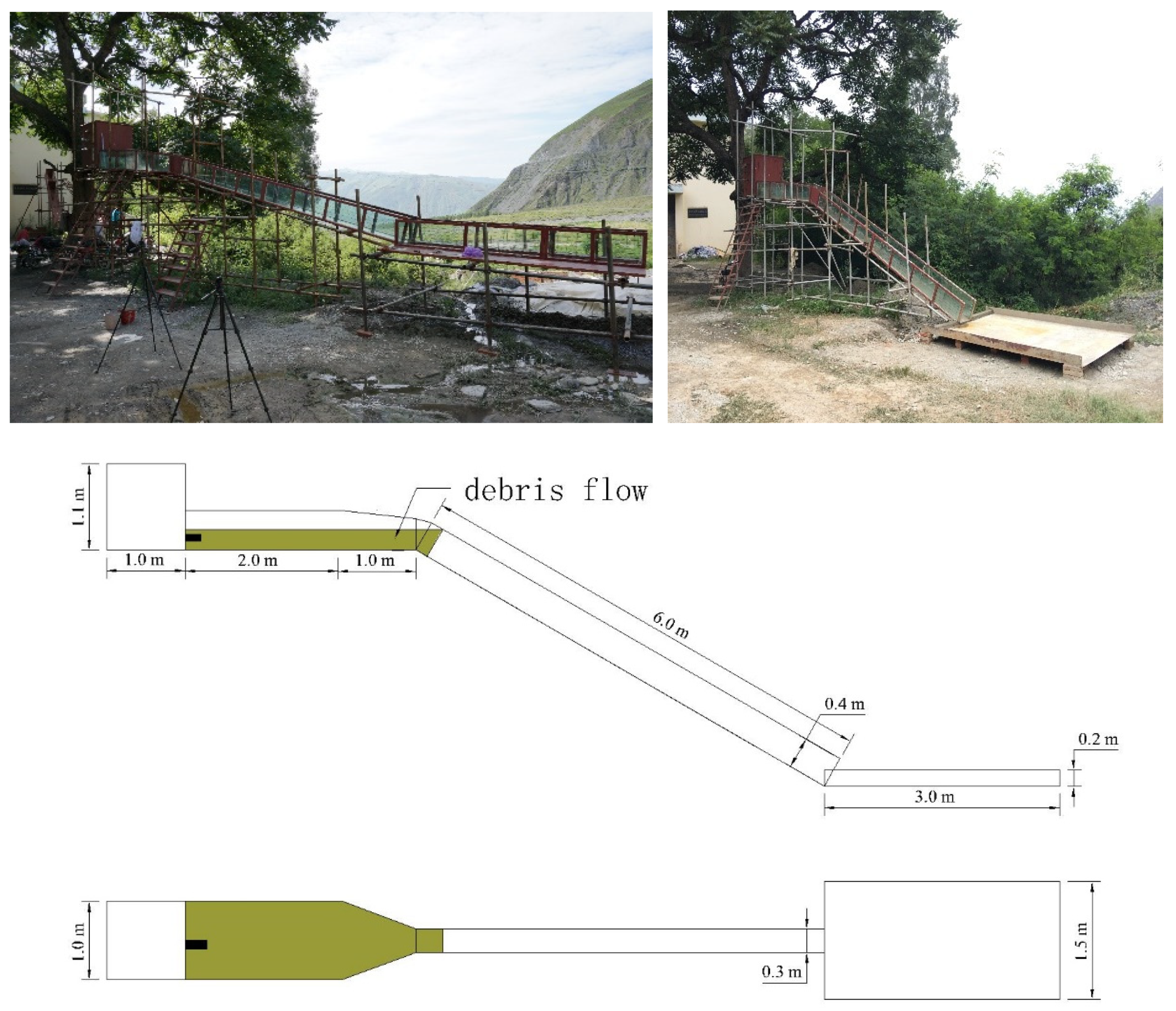
3. Experimental Setup and Boundary Conditions

Figure 1 shows the facility where the experiments for the numerical validation of the method previously described in Section 2 were conducted. This facility is located in the Debris Flow Observation and Research Station at Jiangjia Gully, the largest field research center in China—also known as “the debris flow museum”. For this study, water is stored upstream to the material prepared under multiple configurations and water is always released by opening a steel gate at the velocity of 3 m/s. The flume can then be divided into two parts: (i) a steep upstream reach (6.0 m long and the chute slope can vary from 15° to 40° (always set up at 25° for these experiments); and (ii) a flat-bottomed downstream section (3.0 m long). The slope of the flume’s bed can be manually adjusted.

Details regarding the experimental procedure conducted can be found in [6]. For this study, three slurries were testes with densities ρ = 1400 kg/m³; ρ = 1500 kg/m³ and ρ = 1600 kg/m³. Different layers patterns were selected according to the different configurations displayed in Figure 2. By adding water to the flume, when the water level reached the height of the mixing fluid, the front-end steel gate of the mixing area was released at a speed of 3 m/s. In order to maintain the driving force of the mixtures, the water level behind the mixtures was kept at h = 0.2 m during the experiment.

The experimental configurations chosen to examine the influence of vertical grading patterns on the debris flow formation and propagation are displayed in Figure 2.

There are three configurations: Figure 2a shows the configuration a, with coarse particles as a top layer and fine sediment positioned below them; Figure 2b shows the configuration b, a realistic configuration with the original sediments collected from the Jiangjiagou Valley, fully mixed and distributed along the entire measurement area; Figure 2c shows the configuration c, with coarse particles distributed at the bottom and fine grains on the top of them. For this study, three types of liquid slurries were considered: (i) ρ = 1400 kg/m³, (ii) ρ = 1500 kg/m³, and (iii) ρ = 1600 kg/m³. The slurry rheology coefficient was measured by the MCR301 advanced rotary rheometer manufactured by Anton Paar, Austria [39]. Values of viscosity μ for the fluids simulated are displayed in

Table 1. Experimental conditions (viscosity values and vertical grading patterns) adopted for this study.

Test No.	Factors
	ρ (kg/m3)	Solid Phase Level	μ0 (Pa)	μ1 (Pa·s)	μ2 (Pa·s2)
1	1400	Upper	0.00004	0.0048	0.0197
2	1400	Mixed
3	1400	Bottom
4	1500	Upper	0.00006	0.0051	0.1654
5	1500	Mixed
6	1500	Bottom
7	1600	Upper	0.0001	0.0034	0.8242
8	1600	Mixed
9	1600	Bottom

.

The particle size distribution curves are shown in Figure 3, Ψ stands for the percentage of accumulated mass of particles and d denotes particle size.

4. Simulation and Analysis

By simulating the movement processes of different viscous debris flows, a series of experiments has been completed where free surface heights, fluid velocities, pressures, and shear deformations associated with the movement of the fluid were measured. The numerical simulation was carried out to generate the experimental conditions previously described (Figure 4). The numerical simulation replicated N = 113,054 particles, particle spacing d_p = 0.0025 m, solid particle density ρ_s = 2200 kg/m³, thickness of solid phase h_s = 0.1 m and thickness of liquid phase h_l = 0.1 m for configuration a and c in Figure 2. Similar to the tests conducted on the experimental facility, three different viscosity coefficients for the liquid phases (as shown in Table 1) were selected in the numerical simulation. The inflow conditions were the same as those applied experimentally, and the water level as driving force of the debris flow was kept at 0.2 m for each entire simulation.

Figure 5 represents the free surface values recorded at different times for each of the tests conducted in Table 1, after the debris flow initiation generated by the release of water upstream. The x-axis represents the length L of the debris flow, and the y-axis represents the height H of the debris flow. After 0.7 s, the distance reached by the debris flow (considering all the configurations) is within the range 2.48–2.66 m, and the maximum velocity range is 4.65–5.12 m/s. Authors noticed that when the debris flow has similar viscous properties but for the vertical distribution of different particles, the differences in velocities are not so significant and can considered almost negligible in most of the cases. However, the maximum velocity recorded for configuration b (Shown in Figure 2b correspond to tests 2, 5 and 8 in Figure 5) is similar to the one recorded for configuration a (Shown in Figure 2a and corresponding to tests 1, 4, and 7 in Figure 5), while configuration c (Shown in Figure 2c and corresponding to tests 3, 6, and 9 in Figure 5) was characterized by higher values of velocities and elevations measured. By comparing the shapes of head under different vertical distributions, it was found that for the tests conducted in Table 1, free surface values measured for configuration b fluctuate more than in configuration a and c, demonstrating that this scenario is typical of intermittent debris flows.

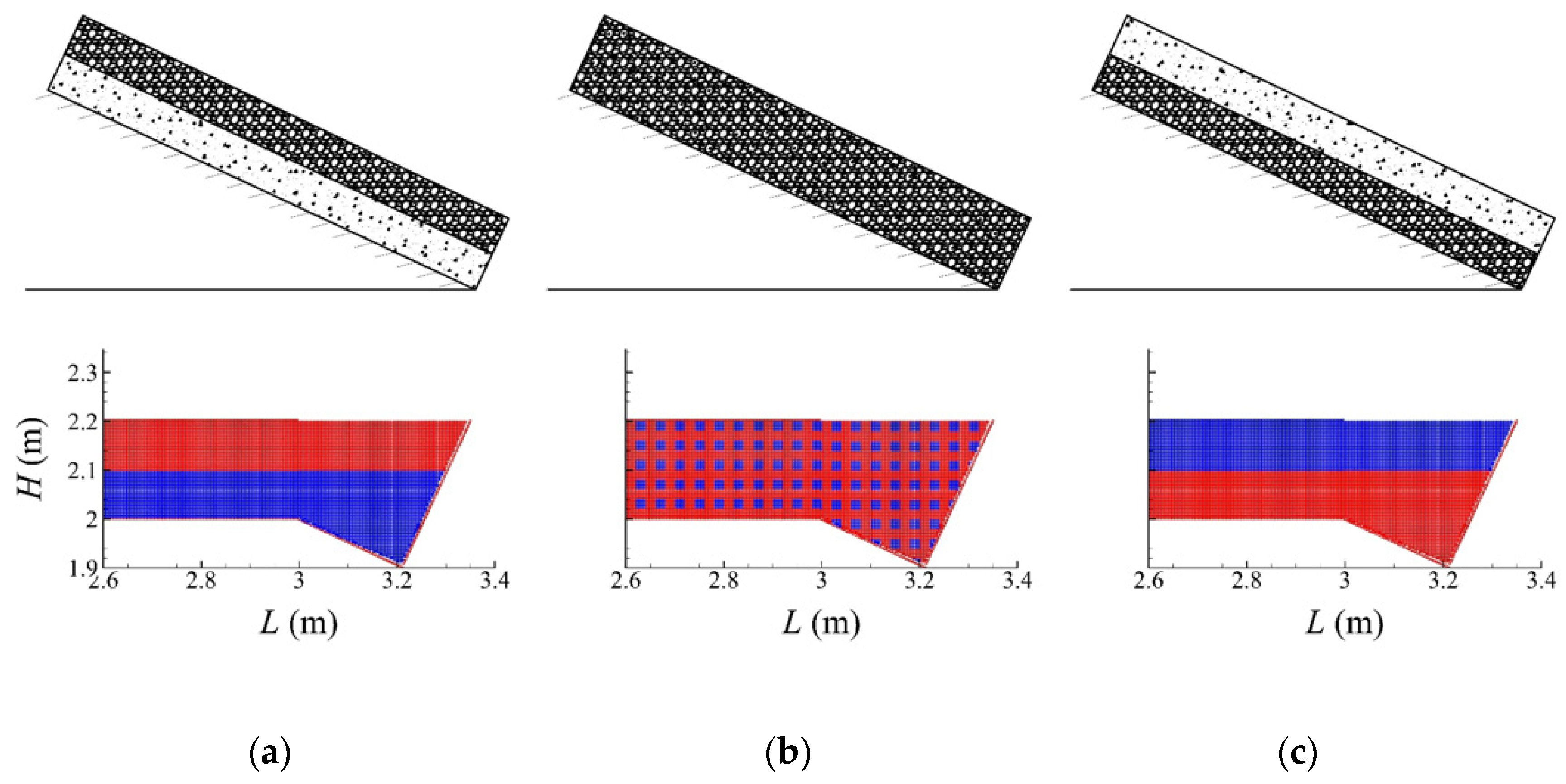
Characterization of Intermittent Debris Flow

In order to study the causes of this phenomenon, the characteristics of the fluid movement processes associated to configuration b were analyzed. Figure 6 shows the evolution of the solid-liquid phase at different locations simulated numerically. Figure 6a shows that in the horizontal region, most of the particles still retain under the laminar form. When moving into the upstream part of the sloped section, the fluid height decreases and the liquid phase group is stretched, as shown in Figure 6b. Then, due to the slope, velocity increases while the fluid height decreases, and different layers of liquid and solid particles will appear almost as parallel mixing within the entire width of the debris flow, as shown in Figure 6c. At this stage, the altering layers interact changing continuously positions demonstrating that mixing processes are taking place and when the mixing is finally completed, the fluctuation amplitude reduce becoming more stable, while the influenced range of the fluctuations can spread over a longer length, as shown in Figure 6d. Figure 6e shows the effect of the liquid phase on the height of the debris flow. It is clear that when liquid particles accumulate due to the mixing phenomena (highlighted as circles in Figure 6e), there is a correspondent decrease of the height of the debris flow (pointed out using arrows in Figure 6e). This inverse relationship is very interesting especially because it demonstrates how the gathering and accumulation of liquid particles tends to appear towards the bottom side of the debris flow layer.

On this basis, the relationship between the moisture content ϕ (the amount of liquid particles divided by the amount of solid particles, $N_l/N_s$), the kinetic energy of particles E_k and the height of the free surface $H$ (related to the potential energy of particles E_p) were calculated for the tests conducted for configuration b. As shown in Figure 7a, the height of the free surface $H$ decreases as the debris flow develops. There is a noticeable correlation between the fluctuation of the free surface associated with the fluctuation of the moisture content. In the regions of L = 1.00–1.38 m and L = 1.82−2.04 m, the height of free surface decreases linearly, and in these two regions, the water content remains in the range 0.2–0.65. The points that obviously exceed this threshold are L = 0.90, L = 1.52, L = 1.6, L = 1.74, and L = 1.80−1.84, and the height of free surface is different from that of linear decline in these areas or vicinity. When the moisture content is within the range 0.20–0.65, the free surface of the debris flow is characterized by a linear change, but when the moisture content exceeds this range, it generates an impact on the free surface.

From Figure 7b, it can be seen that there is a more obvious negative correlation between the particles kinetic energy E_k and the moisture content ϕ. To almost every peak of the kinetic energy E_k (highlighted as green circles in Figure 7b) calculated corresponds a peak of the moisture content ϕ (highlighted as blue circles in Figure 7b), which indicates that kinetic energy E_k and moisture content ϕ interact directly. However, this effect can only be assigned to small-scale portions of the particle kinetic energy fluctuations. Looking at Figure 7b, at the location of L = 1.74 m, the moisture content value corresponds to ϕ = 0.7619 and it is the maximum value measured in this region, and the corresponding kinetic energy E_k records its minimum value. But because of the large kinetic energy of the particles recorded in this region, the corresponding kinetic energy E_k = 5.4848 J is still higher than that recorded at the position of L = 1.64 m in the adjacent one E_k = 0.30263 J.

Figure 8 shows the effect of moisture content ϕ on the kinetic energy E_k and the height of the free surface H on a large scale, for configurations a and c. For both configurations, where the solid phase is located at the top and the bottom, the free surface is greatly affected by the magnitude of the moisture content ϕ, while the kinetic energy E_k is greatly affected by the derivative of moisture content along the length of the slope $\frac{d\phi }{dL}$. However, the fluctuation of the moisture content ∆ϕ along the length L, especially for configuration a where the solid phase is displayed at the top of the debris flow, is relatively small. So the kinetic energy E_k and potential energy E_p curves show relatively large-scale area fluctuations and linear characteristics in comparison to the mixed distribution fluid conditions typical of configuration b.

Finally, the energy conversion curves of fluids with different viscous coefficients were inspected and confronted, as shown in Figure 9. It was found that the gravitational potential energy (E_p = mgH) and the total energy (E₀ = E_k + E_p) of fluids decreases at a similar rate. The difference between three fluids is mainly reflected on kinetic energies. When comparing the set of fluids with the smallest density (ρ = 1400 kg/m³, ${\mu }_0$ = 0.00004, ${\mu }_1$ = 0.0048, and ${\mu }_2$ = 0.0197), results shows that velocity values increase from t = 0.0 s up to t = 0.6 s, reaching almost the highest values, and then the kinetic energy of the three fluids tends to be equal. As the time progresses, the same order appears again in the kinetic energy magnitude arrangement, which is E_k,ρ = 1400 kg/m³ > E_k,ρ = 1500 kg/m³ > E_k,ρ = 1600 kg/m³. This phenomenon is also due to the stronger fluctuation of the less dense fluids and these effects caused by different viscous fluids on debris flow array and collision, and friction forces on debris flow movement, will require further investigation in the future.

5. Summary and Conclusions

Debris flows are a natural phenomenon causing a lot of economical and human losses worldwide. Due to their nature, debris flows travel long distances at high speeds, and the time-space evolution of the relationship between soil and water content strongly affects the propagation stage. Thus, a quantitative modeling of this phenomenon is crucial to design strategies to be adopted to reduce the negative impacts. This paper contributes to this topic through the use of a SPH model investigating multiple combinations of fine and coarse particles with water content.

The SPH model was used to simulate tests conducted in the experimental facility that is located in the Debris Flow Observation and Research Station at Jiangjia Gully, the largest field research center in China—also known as “the debris flow museum”. As previously demonstrated, the SPH model is capable of properly reproducing the main characteristics of debris flows (propagation height and velocity, and more importantly to correctly simulate the time-space evolution of solid and liquid particles during the whole process from initiation to propagation over an impervious/permeable bottom boundary).

Based on the theory of solid-liquid two phase flows, the viscous term in the SPH model was modified to make it suitable for nonhomogeneous viscous debris flows. It was found that the denser the fluid is, the greater are the yield stress and the turbulent viscous coefficient. However for laminar viscous coefficients, the fluid with the density of ρ = 1500 kg/m³ has the largest values. The results obtained can be summarized as follows:

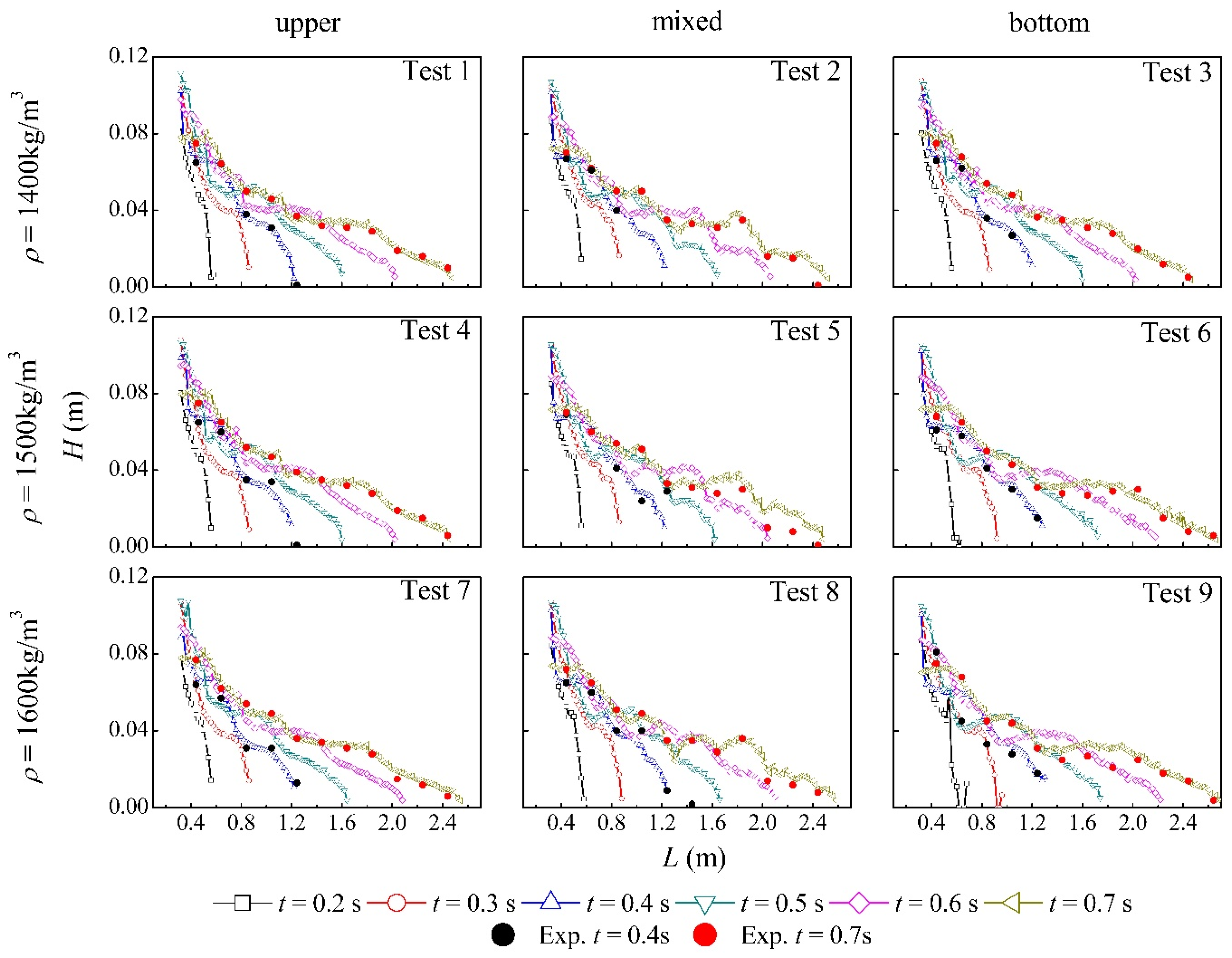
• By comparing the shape and velocity of debris flows under different configurations, it was found that the vertical distribution of particles played a very important role in debris flow fluctuation, with a greater influence than on the viscous coefficient. The third configuration with mixed fine and coarse particles showed to fluctuate more violently, and this outcome confirmed one of the main assumptions for intermittent debris flows.
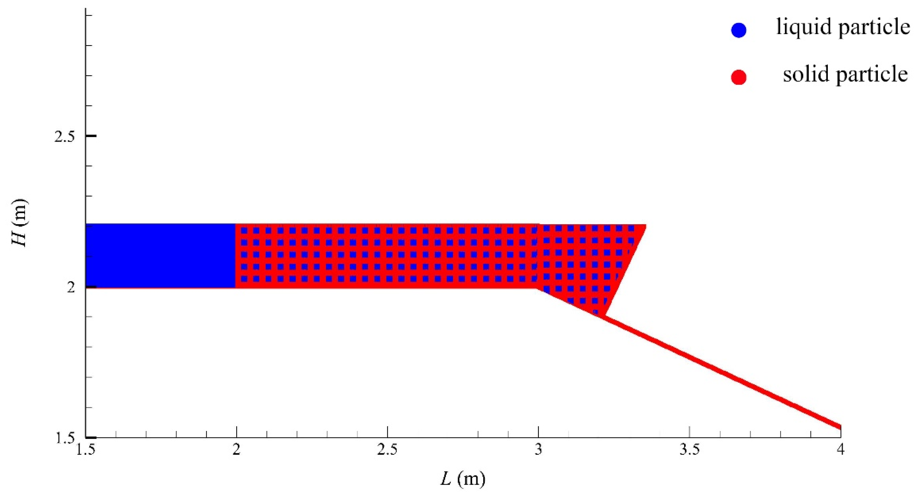
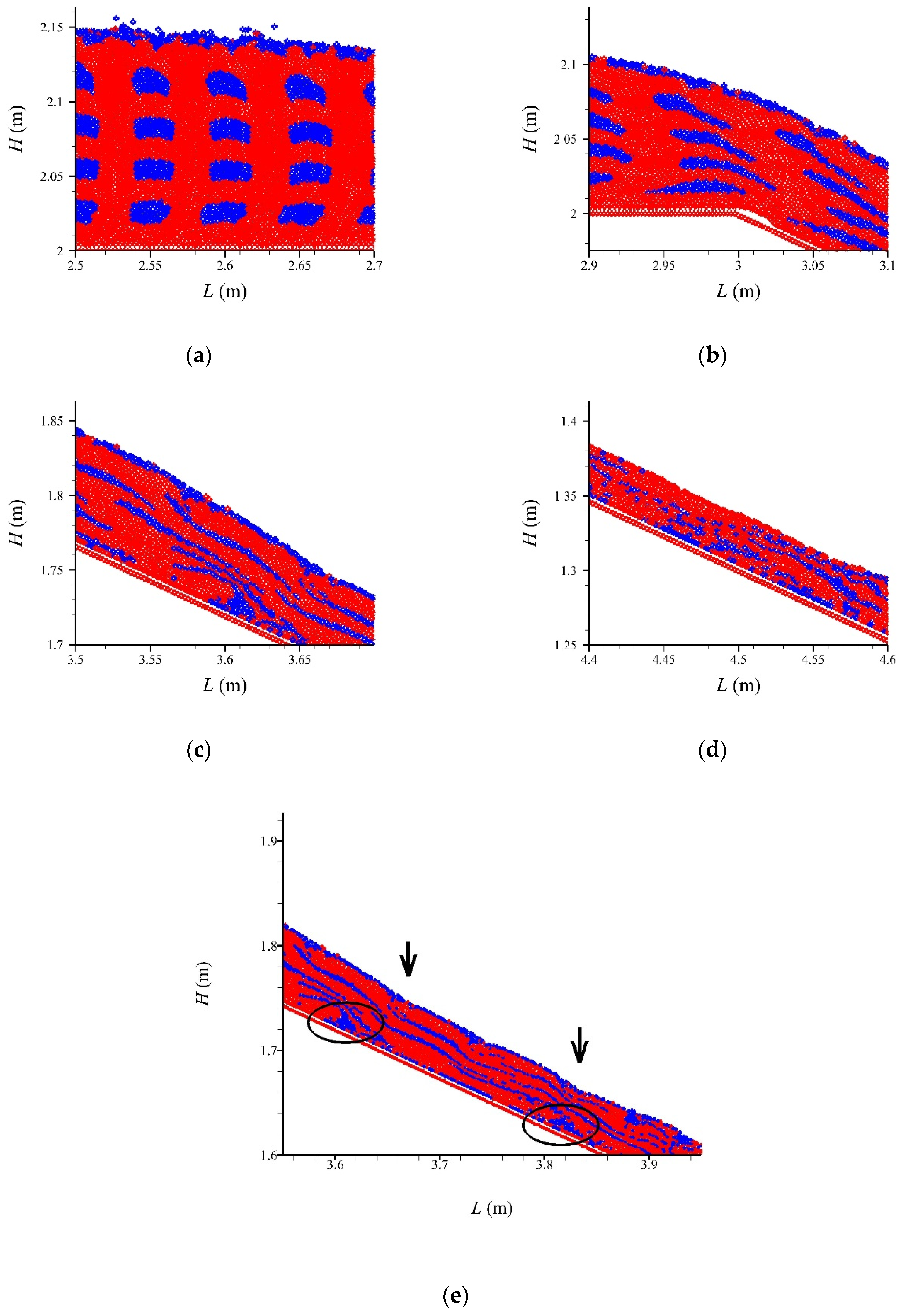
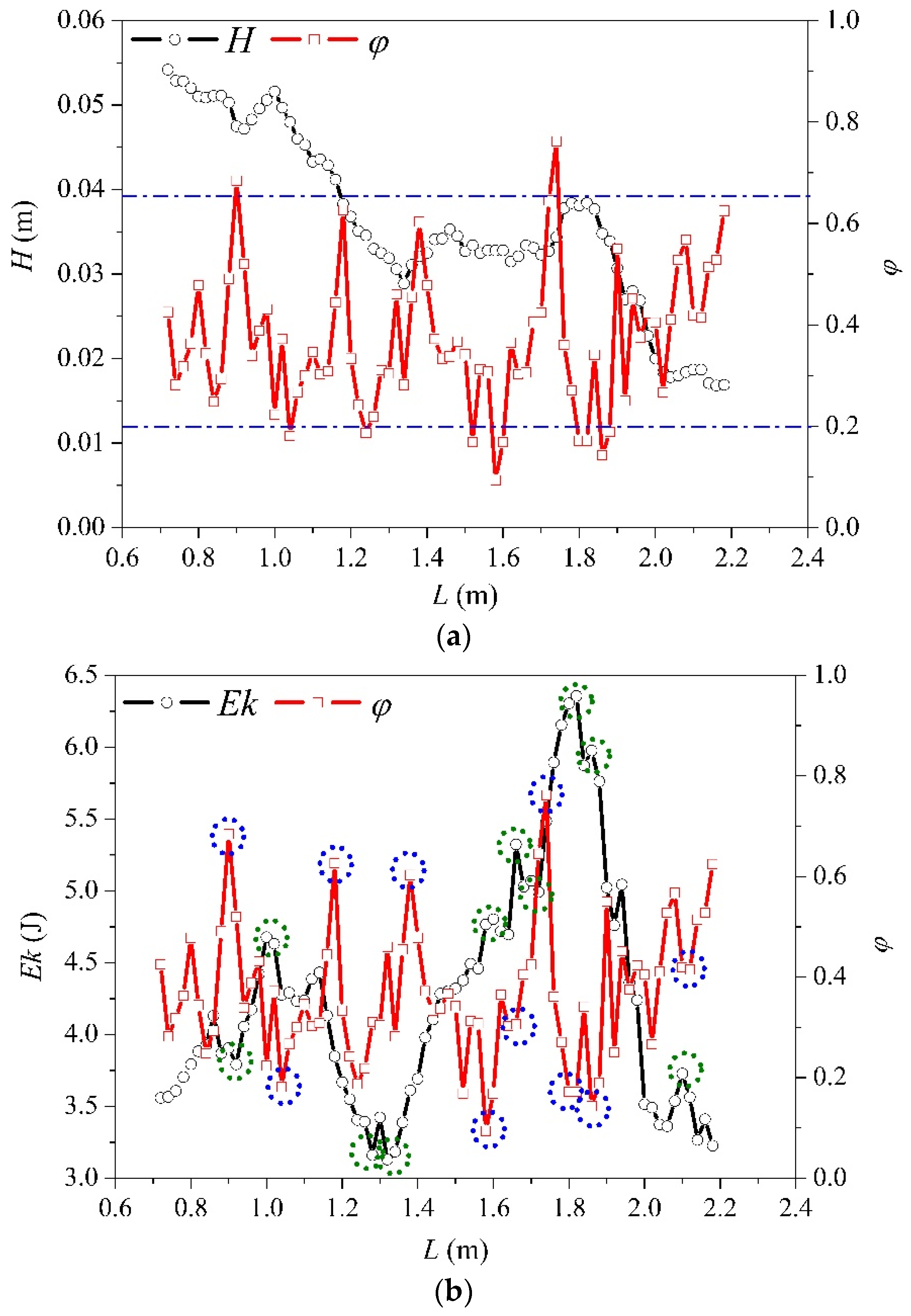
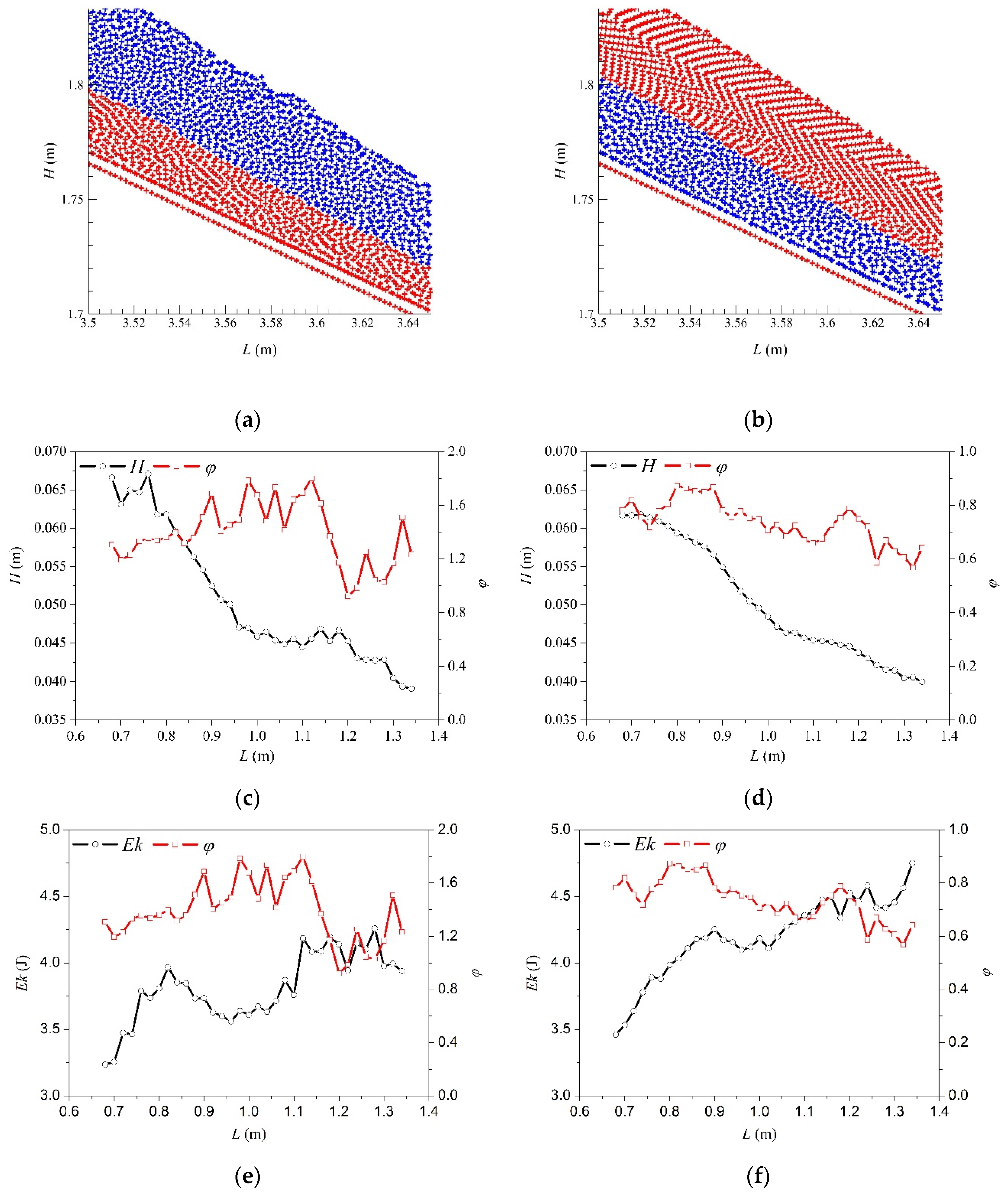
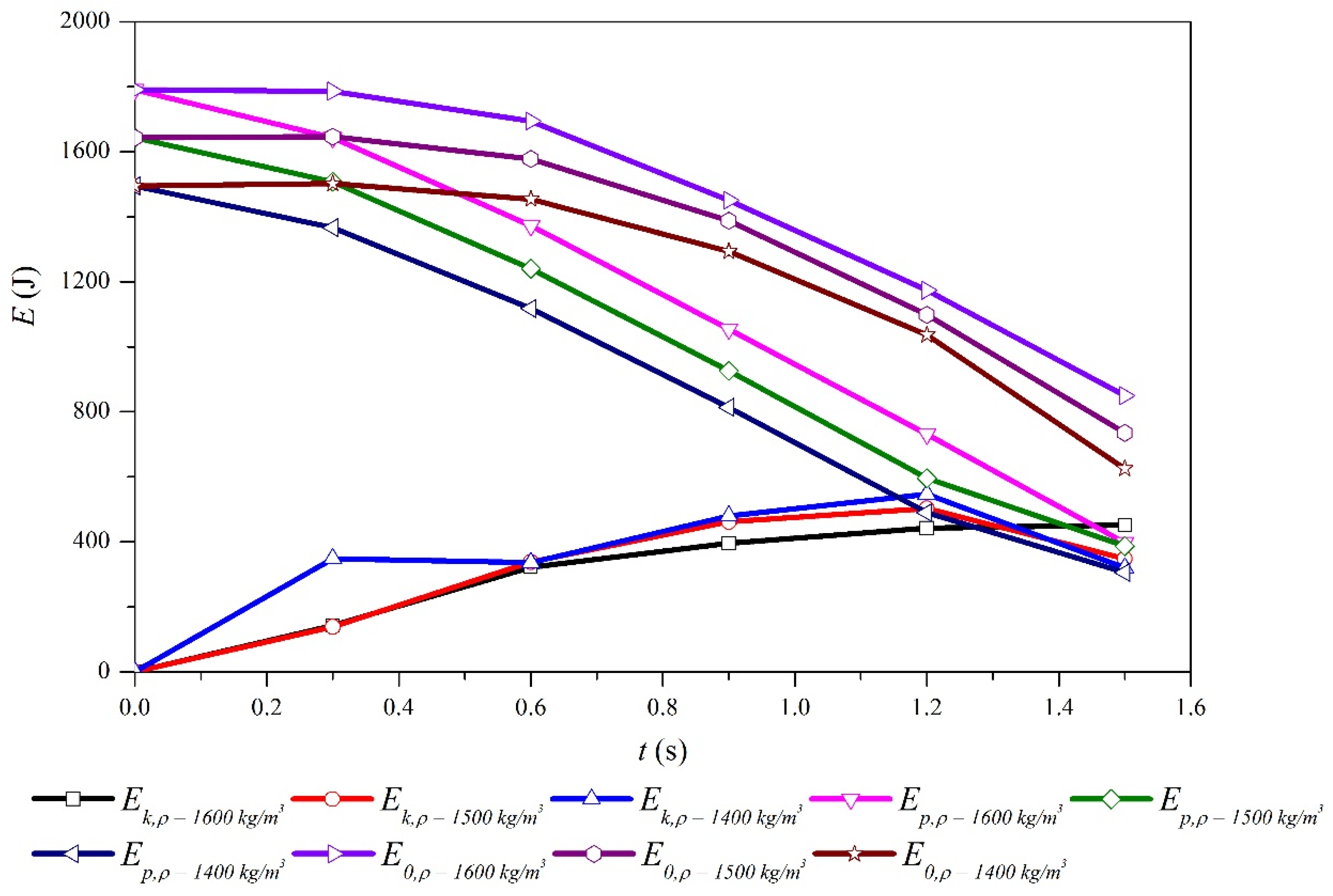
• By analyzing the characteristics of the fluid movement processes, it was found that when the two layers (fine and coarse particles) are mixed with the water, liquid particles tended to gather towards the bottom side of the debris flow causing a correspondent decrease of height. However, this effect could only be observed at small-scale areas. The potential energy was greatly affected by the magnitude of the moisture content, while the kinetic energy was significantly affected by the derivative of moisture content in the L direction.
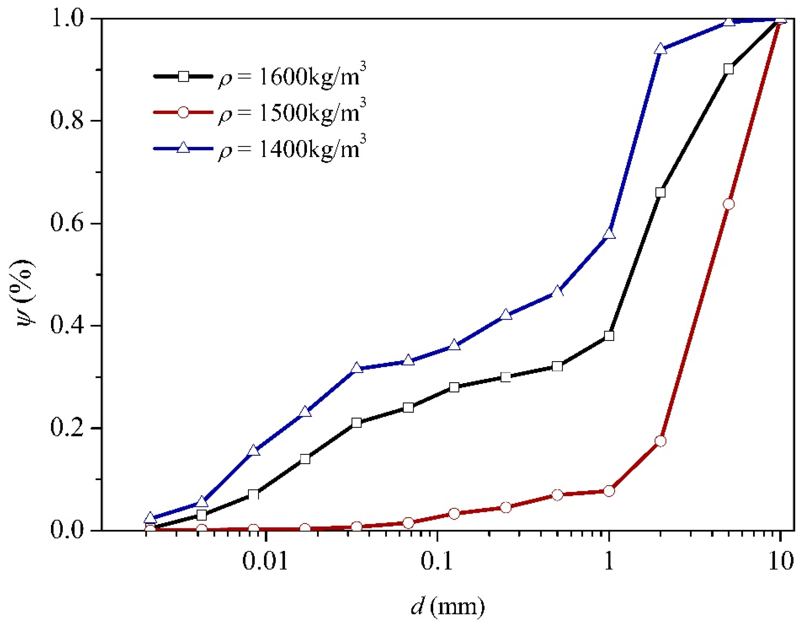
• The differences of the energy conversion curves associated to different viscous coefficients were mainly noticed in kinetic energies. Fluids with smaller densities exhibited higher initiation velocities and higher fluctuations values.

The authors can also confirm that there are still some uncertainties within the results analyzed that could be reduced by the use of either novel physically-based entrainment laws or fully 3D mathematical approaches, which could surely more accurately take into consideration the variation of pore water pressures inside the propagating mass. Therefore, future research will target the development of 3D mathematical models to refine the findings and provide an even better understanding of this very complex natural phenomenon.

References

- Kim, M.I.; Kwak, J.H.; Kim, B.S. Assessment of dynamic impact force of debris flow in mountain torrent based on characteristics of debris flow. Environ. Earth Sci. 2018, 77, 538. [Google Scholar] [CrossRef]
- Zhang, S.; Zhang, L.M. Impact of the 2008 Wenchuan earthquake in China on subsequent long-term debris flow activities in the epicentral area. Geomorphology 2017, 276, 86–103. [Google Scholar] [CrossRef]
- Silhan, K.; Tichavsky, R. Recent increase in debris flow activity in the Tatras Mountains: Results of a regional dendogeomorphic reconstruction. CATENA 2016, 143, 221–231. [Google Scholar] [CrossRef]
- Brandinoni, F.; Mao, L.; Recking, A.; Rickenmann, D.; Turowski, J.M. Morphodynamics of steep mountain channels. Earth Surf. Process. Landf. 2015, 40, 1560–1562. [Google Scholar] [CrossRef]
- Takahashi, T.; Das, D.K. Debris Flow: Mechanics, Prediction and Countermeasures; CRC Press: London, UK, 2014. [Google Scholar]
- Shu, A.P.; Tian, L.; Wang, S.; Rubinato, M.; Zhu, F.Y.; Wang, M.Y.; Sun, J.T. Hydrodynamic characteristics of the formation processes for non-homogeneous debris-flow. Water 2018, 10, 452. [Google Scholar] [CrossRef]
- Liu, J.J.; Li, Y. A review of study on drag reduction of viscous debris flow residual layer. J. Sedim. Res. 2016, 3, 72–80. (In Chinese) [Google Scholar]
- Johnson, A.M. Physical Processes in Geology; Freeman Cooper & Company: San Francisco, CA, USA, 1970. [Google Scholar]
- Bagnold, R.A. Experiments on a gravity-free dispersion of large solid spheres in a Newtonian fluid under shear. Proc. R. Soc. Lond. Ser. A 1954, 22, 49–63. [Google Scholar]
- Takahashi, T. Mechanical characteristics of debris flow. J. Hydraul. Div. Am. Soc. Civ. Eng. 1978, 104, 1153–1169. [Google Scholar]
- Chen, C.L. Generalized viscoplastic modelling of debris flow. J. Hydraul. Div. Am. Soc. Civ. Eng. 1988, 114, 237–258. [Google Scholar] [CrossRef]
- Chen, C.L. General solutions for viscoplastic debris flow. J. Hydraul. Div. Am. Soc. Civ. Eng. 1988, 114, 259–282. [Google Scholar] [CrossRef]
- O’Brien, J.S.; Julien, P.Y. Laboratory analysis of mudflow properties. J. Hydraul. Div. Am. Soc. Civ. Eng. 1988, 114, 877–887. [Google Scholar] [CrossRef]
- O’Brien, J.S.; Julien, P.Y.; Fullerton, W.T. Two-dimensional water flood and mudflow simulation. J. Hydraul. Div. Am. Soc. Civ. Eng. 1993, 119, 244–261. [Google Scholar] [CrossRef]
- Dai, Z.; Huang, Y.; Cheng, H.; Xu, Q. 3D Numerical modeling using smoothed particle hydrodynamics of flow-like landslide propagation triggered by the 2008 Wenchuan earthquake. Eng. Geol. 2014, 180, 21–33. [Google Scholar] [CrossRef]
- Hosseini, S.M.; Manzari, M.T.; Hannani, S.K. A fully explicit three-step SPH algorithm for simulation of non-Newtonian fluid flow. Int. J. Numer. Methods Heat Fluid Flow 2007, 17, 715–735. [Google Scholar] [CrossRef]
- Rodriguez-Paz, M.X.; Bonet, J. A corrected smooth particle hydrodynamics method for the simulation of debris flows. Numer. Methods Part Differ. Equ. 2004, 20, 140–163. [Google Scholar] [CrossRef]
- Savage, S.B.; Hutter, K. The dynamics of avalanches of granular materials from initiation to run out. Acta Mech. Sin. 1991, 86, 201–223. [Google Scholar] [CrossRef]
- Trunk, F.J.; Dent, J.D.; Lang, T.E. Computer modeling of large rock slides. J. Geotech. Eng. 1986, 112, 348–360. [Google Scholar] [CrossRef]
- Iverson, R.M. The physics of debris flows. Rev. Geophys. 1997, 35, 245–296. [Google Scholar] [CrossRef]
- Xenakis, A.M.; Lind, S.J.; Stansby, P.K.; Rogersb, B.D. An incompressible SPH scheme with improved pressure predictions for free-surface generalised Newtonian flows. J. Non-Newton. Fluid Mech. 2015, 218, 1–15. [Google Scholar] [CrossRef]
- Springel, V.; Hernquist, L. Cosmological smoothed particle hydrodynamics simulations: A hybrid multiphase model for star formation. Mon. Not. R. Astron. Soc. 2003, 339, 289–311. [Google Scholar] [CrossRef]
- Gómez-Gesteira, M.; Dalrymple, R.A. Using a three-dimensional Smoothed Particle Hydrodynamics method for wave impact on a tall structure. J. Waterw Port Coast. 2004, 130, 63–69. [Google Scholar] [CrossRef]
- Flebbe, O.; Muenzel, S.; Herold, H.; Riffert, H. Smoothed Particle Hydrodynamics: Physical viscosity and the simulation of accretion disks. Astrophys. J. 1994, 431, 754–760. [Google Scholar] [CrossRef]
- Lucy, L.B. A numerical approach to the testing of the fission hypothesis. Astron. J. 1977, 82, 1013–1024. [Google Scholar] [CrossRef]
- Liu, G.R.; Liu, M.B. Smoothed Particle Hydrodynamics: A Mesh-Free Particle Method; World Scientific Publishing Company: Singapore, 2003; pp. 27–33. [Google Scholar]
- Monaghan, J.J. Smoothed particle hydrodynamics. Annu. Rev. Astron. Astrophys. 1992, 30, 543–574. [Google Scholar] [CrossRef]
- Gingold, R.A.; Monaghan, J.J. Smoothed particle hydrodynamics: Theory and application to non-spherical stars. Mon. Not. R. Astron. Soc. 1977, 181, 375–389. [Google Scholar] [CrossRef]
- Gingold, R.A.; Monaghan, J.J. Kernel estimates as a basis for general particle methods in hydrodynamics. J. Comput. Phys. 1982, 46, 429–453. [Google Scholar] [CrossRef]
- Monaghan, J.J. Particle methods for hydrodynamics. Comput. Phys. Rep. 1985, 3, 71–124. [Google Scholar] [CrossRef]
- Fulk, D.A.; Quinn, D.W. An Analysis of 1-D Smoothed Particle Hydrodynamics kernels. J. Comput. Phys. 1996, 126, 165–180. [Google Scholar] [CrossRef]
- Colagrossi, A.; Landrini, M. Numerical simulation of interfacial flows by Smoothed Particle Hydrodynamics. J. Comput. Phys. 2003, 191, 448–475. [Google Scholar] [CrossRef]
- Bose, A.; Carey, G.F. Least-squares p-r finite element methods for incompressible non-Newtonian flows. Comput. Methods Appl. Mech. 1999, 180, 431–458. [Google Scholar] [CrossRef]
- Wood, D. Collapse and fragmentation of isothermal gas clouds. Mon. Not. R. Astron. Soc. 1981, 194, 201–218. [Google Scholar] [CrossRef][Green Version]
- Bonet, J.; Lok, T.S.L. Variational and momentum preservation aspects of Smooth Particle Hydrodynamic formulations. Comput. Method Appl. Mech. 1999, 180, 97–115. [Google Scholar] [CrossRef]
- Loewenstein, M.; Mathews, W.G. Adiabatic particle hydrodynamics in three dimensions. J. Comput. Phys. 1986, 62, 414–428. [Google Scholar] [CrossRef]
- Shao, S.; Lo, E.Y.M. Incompressible SPH method for simulating Newtonian and non-Newtonian flows with a free surface. Adv. Water Resour. 2003, 26, 787–800. [Google Scholar] [CrossRef]
- Lo, E.Y.M.; Shao, S.D. Simulation of near-shore solitary wave mechanics by an incompressible SPH method. Appl. Ocean Res. 2002, 24, 275–286. [Google Scholar]
- Yang, H.J.; Wei, F.Q.; Hu, K.H. Determination of the maximum packing fraction for calculating slurry viscosity of debris flow. J. Sediment. Res. 2018, 3, 382–390. [Google Scholar]