Comparing Meteorological Data Sets in the Evaluation of Climate Change Impact on Hydrological Indicators: A Case Study on a Mexican Basin

Abstract

This study evaluates the choice of the meteorological data set in the simulation of the streamflow of a Mexican basin, in the bias correction of climate simulations, and in the climate change impact on hydrological indicators. The selected meteorological data sets come from stations, two interpolated data sets and one reanalysis data set. The climate simulations were taken from the five-member ensemble from the second generation Canadian Earth System Model (CanESM2) under two representative concentration pathways (RCPs), for a reference period (1981–2000) and two future periods (2041–2060 and 2081–2100). The selected lumped hydrological model is GR4J, which is a daily lumped four-parameter rainfall-runoff model. Firstly, the results show that GR4J can be calibrated and validated with the meteorological data sets to simulate daily streamflow; however, the hydrological model leads to different hydrological responses for the basin. Secondly, the bias correction procedure obtains a similar relative climate change signal for the variables, but the magnitude of the signal strongly varies with the source of meteorological data. Finally, the climate change impact on hydrological indicators also varies depending on the meteorological data source, thus, for the overall mean flow, this uncertainty is greater than the uncertainty related to the natural variability. On the other hand, mixed results were found for high flows. All in all, the selection of meteorological data source should be taken into account in the evaluation of climate change impact on water resources.

1. Introduction

Evaluation of the climate change impact on water resources is an important issue in hydrology science, as the expected changes in the precipitation and temperature patterns would affect the availability of water for the population as well as the ecosystems. Additionally, it is expected that the climate change impact on the hydrological regimes would lead to changes in average runoffs. For instance, Arnell et al. [1] argue that runoffs would increase in high latitudes, but they would decrease in other regions, such as Central and South America. The evaluations of the climate change impact on hydrology must deal with several uncertainties, such as the General Climate Model (GCM), the emission scenario or the representative concentration pathway (RCP), the statistical bias correction procedure, and the hydrological model [2,3,4,5,6,7,8,9,10].

On the other hand, the evaluation of the impact of climate change on water resources requires high-quality meteorological records in order to calibrate and validate the hydrological models, and to bias-correct climate simulations. To that concern, the Intergovernmental Panel on Climate Change (IPCC) argues that historical records in many regions are poor, especially for those more vulnerable to climate change; thus, it recommends further research to integrate observations into processed gridded products [11].

Precipitation data issued from gridded meteorological datasets present important differences among them. Such differences lead to uncertainty in runoff simulation. For instance, Fekete et al. [12] evaluated six monthly gridded precipitation datasets in runoff evaluation and found a high uncertainty in the estimation of runoff in semiarid regions. Biemans et al. [13] evaluated seven gridded datasets and found great uncertainty in the estimation of simulated runoff over 95 basins, which led authors to conclude that the range of uncertainty in input data has a critical influence on hydrological simulations and must be taken into consideration upon communication of results. Geritana et al. [14] evaluated six gridded datasets in runoff evaluation, and identified underestimation of precipitation which led to misrepresentation of runoff. Other studies have found good results when gridded data is used to simulate streamflow with semi-distributed [15] or lumped hydrological models [16].

Nonetheless, few studies have considered the uncertainty of meteorological dataset in the evaluation of climate change impact on hydrology. For instance, the study of Gao et al. [17] assessed the uncertainty related to data source in the bias correction of climate simulations for the evaluation of climate change impact on annual mean streamflow. Meteorological sources included data from weather stations and from two processed gridded data sets. The authors found that meteorological data source uncertainty was smaller than the uncertainty related to GCM, but larger than uncertainty associated to RCP.

The aims of this study are: firstly, to evaluate different meteorological datasets in the calibration and validation of a hydrological model in the simulation of daily streamflow; secondly, to assess the choice of meteorological data set in the bias correction of climate simulations; and finally, to evaluate this uncertainty in the evaluation of the climate change impact on hydrological indicators. Uncertainty associated with the choice of meteorological data set is also compared to uncertainty related to natural climate variability.

The manuscript is organized as follows: Section 2 describes the basin under study, the meteorological data sets, the climate simulations, the bias correction method and the hydrological model and indicators; Section 3 shows the evaluation of meteorological datasets in the reference period, the performance of the hydrological model, and the evaluation of uncertainty related to the choice of meteorological data set in the bias correction of climate simulations and in the impact of climate change on the hydrological indicators; Section 4 discusses results; and finally, Section 5 concludes.

2. Materials and Methods

The model chain in this study consists of global climate model outputs statically bias-corrected and downscaled to feed a hydrological model. Since we aim to compare the use of different meteorological datasets in the evaluation of climate change impact on water resources, the bias correction of climate outputs and the hydrological model calibration and validation procedure were performed with each of the four selected data sets. This section describes the study basin, the meteorological and climate data, the bias correction procedure, the hydrological model, and the selected hydrological indicators.

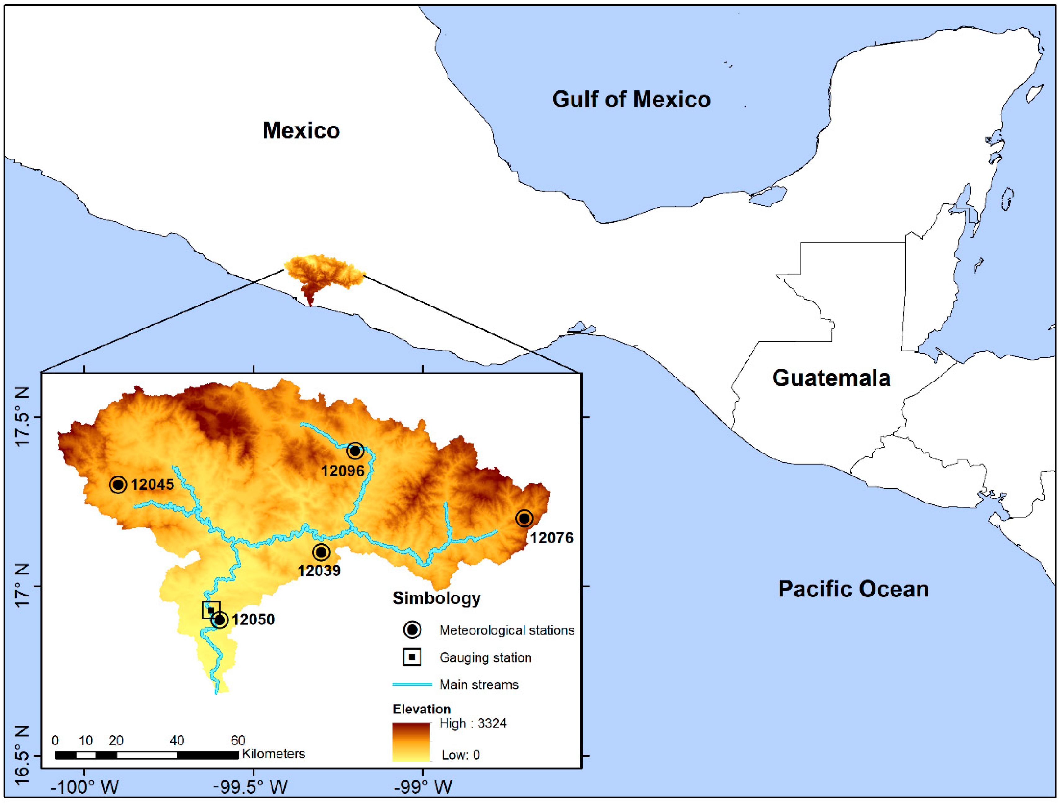
2.1. The Study Basin and the Meteorological Data Sets

The study basin is the Papagayo River Basin, located in south Mexico (Figure 1). The basin has its farthest headwater in the Sierra Madre del Sur mountain chain and discharges into the Pacific Ocean. The basin covers an area of 7067 km² and is located over a Tropical Savannah (Aw) climate region [18]. The mean annual precipitation is 1540 mm and the mean temperature is 20.5 °C evaluated for the 1981–2000 period. The discharge data come from the National Surface Water data set [19] for La Parota gauging station over the same period. The Papagayo River’s flow peaks in September (434 m³ s⁻¹), while its lowest discharge is in February (30 m³ s⁻¹).

Meteorological data (daily precipitation and temperature) were obtained from four data sets (

Table 1. Meteorological data sets selected for this study.

I.D.	Description	Source
data 1	Observation from five meteorological stations (Figure 1)	Servicio Meteorológico Nacional (SMN) via CICESE (Ensenada Center for Scientific Research and Higher Education) website [23]
data 2	Interpolated meteorological data (resolution of 1/16°)	NOAA (National Oceanic and Atmospheric Administration) website [24]
data 3	Interpolated meteorological data (resolution of 1/8°)	CICESE website [23]
data 4	Climate Forecast System reanalysis (CFSR; resolution of 1/2°)	Texas University website [25]

) that include station observations, interpolated meteorological data and reanalysis data for the common 1981–2000 period. Meteorological observations (data 1) were obtained from five SMN (Servicio Meteorológico Nacional) stations located in the basin (Figure 1). In addition, two gridded processed data sets were also considered: data 2 were taken from the data set for Mexico, the U.S.A., and Southern Canada presented by Livneh et al. [20], and data 3, which is the interpolated data set for Mexico introduced by Zhu et al. [21]. Both data sets were built from SMN data; moreover, data 2 incorporates a topographic adjustment that takes into account mountain precipitation. Finally, data 4 was taken from the NCEP (U.S. National Centers for Environmental Prediction) reanalysis [22], which is a gridded data set from a numerical weather prediction model that incorporates observed meteorological data.

Gridded data sets have different resolutions as shown in Table 1. In this study, the selected hydrological model is a lumped model: thus, for a given variable, the model is fed with one series that describes the basin as a whole. Therefore, average daily precipitation and temperature were obtained for each dataset. For the gridded data sets, average precipitation was computed considering the grid points within the basin. For data 1, the average precipitation was obtained following the Thiessen Polygon Method [26]. The basin is located in a mountainous area, thus, an interesting technique to explore is the modification of the Thiessen method proposed by Panagoulia et al. [27], which takes into account the station elevation.

2.2. Climate Simulations and the Bias Correction Method

For this study, the five-member ensemble from the second generation Canadian Earth System Model CanESM2 [28] under two representative concentration pathways (RCP 4.5 and RCP 8.5) was considered. Climate simulations were obtained for a reference period (1981–2000) and two future periods (2041–2060 and 2081–2100). The five-member ensemble climate simulation was selected to provide an estimation of natural climate variability. This natural variability can be estimated by repeating a climate change experiment using a given GCM several times when only the initial conditions are changed by small perturbations [29]. Therefore, the natural variability is irreducible even if perfect models would be available [6], and it is used in this study as a baseline to compare the uncertainty induced by the meteorological datasets.

Climate simulations have systematic biases (i.e., differences in observations within the historical period) that should be corrected before their use in hydrological models in order to provide consistent hydrological simulations [7]. In this study, the daily translation method [30] was selected to bias-correct precipitation and temperature simulations. The method establishes, in a first step, a relationship (correction factors) between the climate model simulations and the meteorological variables in the historical period (at different percentiles). On a second step, correction factors are applied to correct climate simulation in future periods. The daily translation method is applied on a monthly basis, and 50 percentiles are calculated for each month. The corrected daily temperature and precipitation in the historical reference (ref) period are computed as follows:

$$T_{corr\left(d\right)}^{ref}=T_{sim\left(d\right)}^{ref}+\left(T_{obs\left(m,q\right)}^{ref}-T_{sim\left(m,q\right)}^{ref}\right),$$

(1)

$$P_{corr\left(d\right)}^{ref}=P_{sim\left(d\right)}^{ref}\left(\frac{P_{obs\left(m,q\right)}^{ref}}{P_{sim\left(m,q\right)}^{ref}}\right).$$

(2)

where T_corr and P_corr are the bias-corrected temperature and precipitation, respectively. The indexes correspond to percentile (q), daily (d) time steps, raw climate simulations (sim), and observations (obs) or other meteorological data source. For the future period (fut), corrected precipitation and temperature are obtained through:

$$T_{corr\left(d\right)}^{fut}=T_{sim\left(d\right)}^{fut}+\left(T_{obs\left(m,q\right)}^{ref}-T_{sim\left(m,q\right)}^{ref}\right),$$

(3)

$$P_{corr\left(d\right)}^{fut}=P_{sim\left(d\right)}^{fut}\left(\frac{P_{obs\left(m,q\right)}^{ref}}{P_{sim\left(m,q\right)}^{ref}}\right).$$

(4)

The monthly correction factors were computed for the five-member ensemble average, upon which the correction was performed for each individual member in order to conserve the inter-member variability.

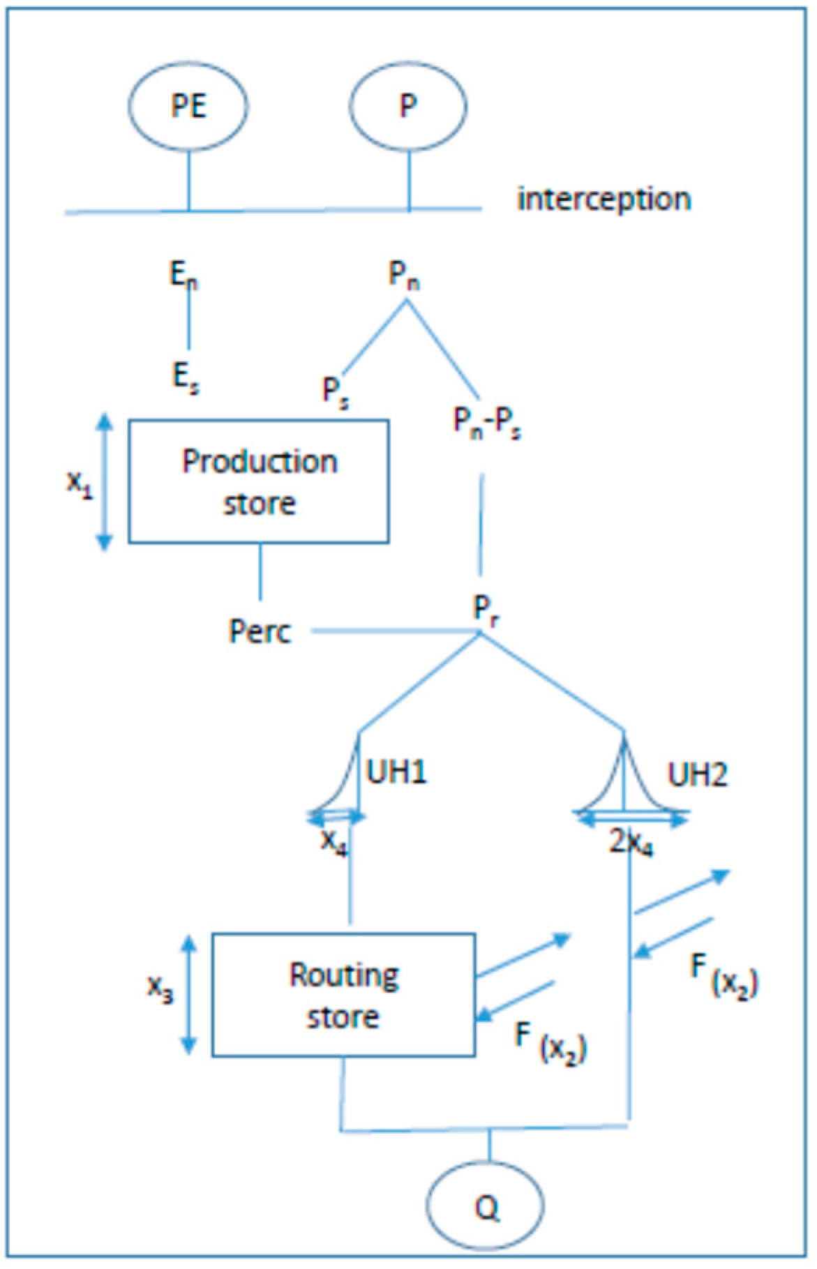
2.3. The Hydrological Model and Hydrological Indicators

The lumped conceptual hydrological model GR4J (Modèle du Génie Rural à 4 paramètres Journalier) was selected for this study. The GR4J model is a daily lumped four-parameter rainfall-runoff model developed by Perrin et al. [31]. Figure 2 shows the model structure. Input variables are daily precipitation (P) and potential evapotranspiration (PE). For this study, the PE was computed with the formulation proposed by Oudin et al. [32], which is based on mean temperature and extraterrestrial radiation. The hydrology in GR4J is simulated as follows: first, the model calculates the net rainfall (P_n) or the net evapotranspiration capacity (E_n) with the subtraction of PE from precipitation. In case P_n is not zero, a portion of the precipitation (P_s) goes into the production store. If, on the other hand, E_n is not zero, a quantity E_s is computed as a function of the water that evaporates from the store. The percolation (perc) from the production store meets the runoff directly. Water quantity P_r is divided into two flow components routed by two unit hydrographs, UH1 and UH2. A groundwater exchange term (F) describes water imports and exports. Four parameters are calibrated in GR4J: x₁, the maximum capacity of the production store; x₂, the groundwater exchange coefficient; x₃, one day ahead maximum capacity of the routing store; and x₄, the time base of the unit hydrograph. A detailed description of the model structure is presented in Perrin et al. [31].

The hydrological indicators selected in this study are: the overall mean flow (OMF), which is the mean daily flow for a given period; the two-year (HF2) and the 10-year (HF10) return period high flow. To evaluate high flow indicators, it was assumed that the time series follow the log Pearson III probability density function.

In this study, a five-member ensemble climate simulation was selected to evaluate the impact of climate change on hydrological indicators. The relative changes on hydrological indicators were performed with permutations as in Velázquez et al. [6]. This method assumes that each member of the ensemble (in the historical reference and future periods) is an independent proxy of the climate. Therefore, the permutation allows comparing the future of a given member in the presence of all members.

The relative differences of the hydrological indicators (∆ij) are computed as follows:

$${∆}_{ij}=\frac{I_i^{fut}-I_j^{ref}}{I_j^{ref}}$$

(5)

where the i and j subscripts represent the climate model simulations (issued from the five-member ensemble) used to compute the hydrological indicators. Hence, we obtain 25 values of relative differences which express the climate change signal (CCS) on a given hydrological indicator.

3. Results

This section shows, firstly, the comparison between meteorological datasets in the historical reference period; secondly, the performance of the hydrological model calibrated and validated with each dataset; and finally, the climate change signal on meteorological variables and hydrological indicators.

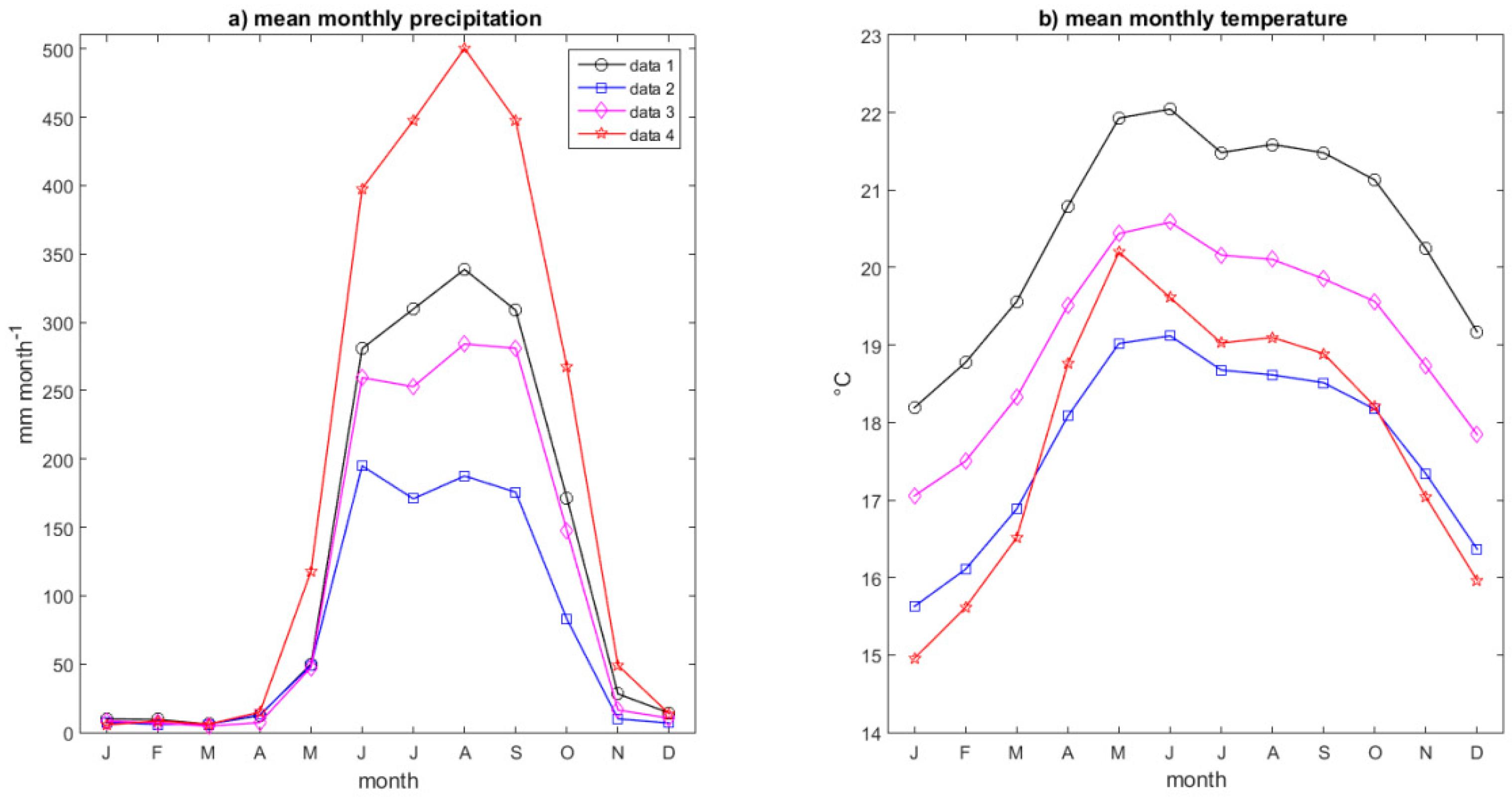
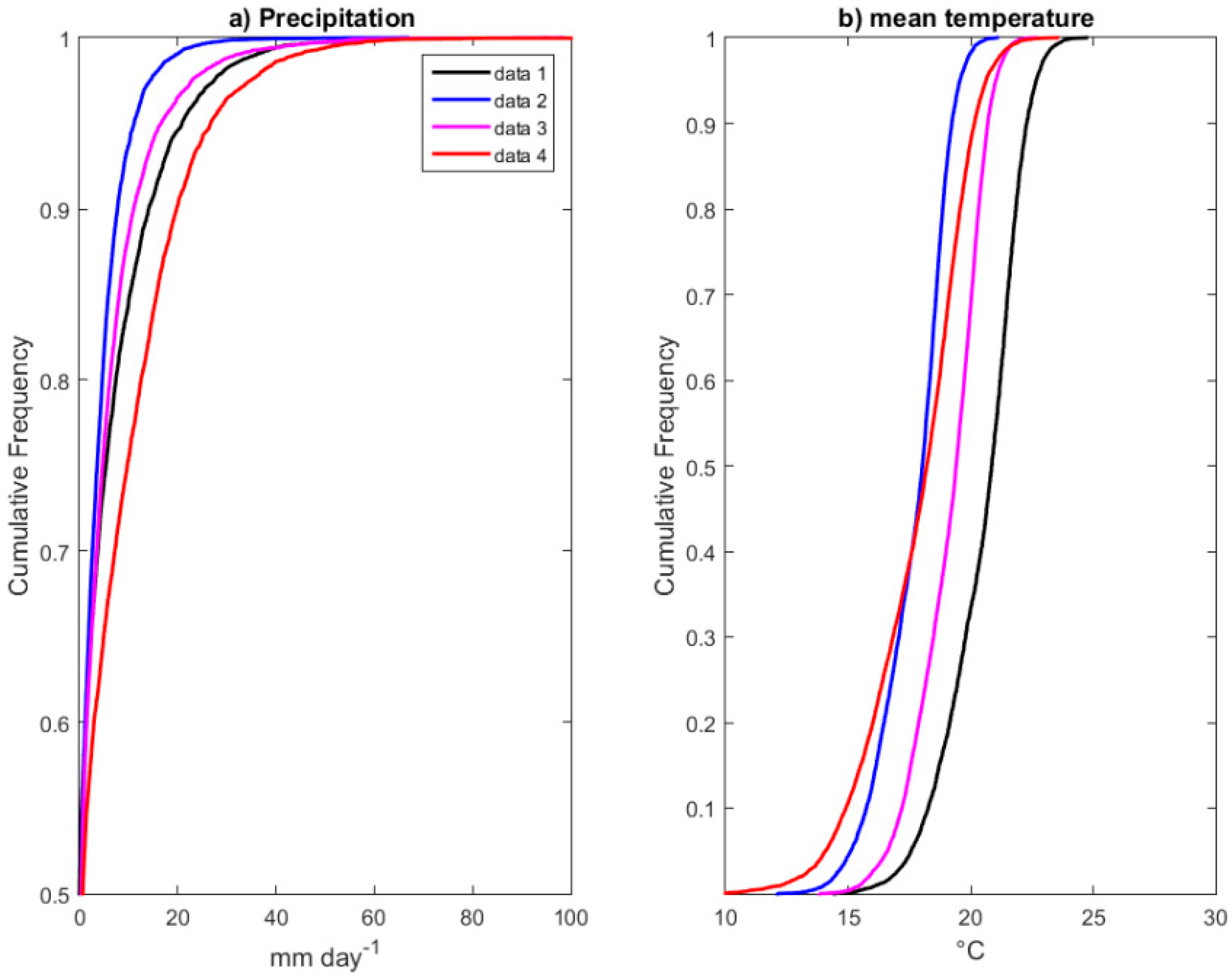
3.1. Comparison of Meteorological Data Sets in a Reference Period

Figure 3 shows the mean monthly precipitation and temperature as evaluated with the four data sets for the period 1981–2000. Compared to station data (data 1), it can be noted that for dry months (November to April) the mean precipitation evaluated with the other data sets is very similar. However, in wet months (May to October), precipitation is underestimated in the processed gridded precipitation (data 2 and data 3) and overestimated in the reanalysis data (data 4). For example, observed precipitation in August shows a value of 338 mm, while showing a value of 187 mm, 284, and 500 mm for data 2, data 3, and data 4, respectively. Additionally, Figure 3a shows differences in the annual cycle for data 2 and data 3 as July precipitation is lower than June and August precipitation.

Regarding the mean monthly temperature, Figure 3b shows a general underestimation of temperature; for instance, the difference in the observed temperature (data 1) in the warmest month (June) is 2.9 °C, 1.4 °C, and 2.4 °C for data 2, data 3, and data 4, respectively. Additionally, Figure 3b shows that the reanalysis (data 4) estimates the highest temperature in May rather than June.

Figure 4 shows the empirical cumulative distribution functions for daily precipitation and mean temperature over the study basin, while

Table 2. Selected percentiles (pctl) for daily precipitation and mean temperature computed with the meteorological data sets for the period 1981–2000.

pctl	Precipitation (mm day−1)
	data 1	data 2	data 3	data 4
50	0	0.33	0.37	0.67
75	5.39	3.59	4.66	9.73
90	20.86	11.13	16.64	26.64
	Temperature (°C)
10	18.28	15.75	17.19	14.91
50	20.87	18.03	19.40	18.20
90	22.30	19.23	20.69	20.15

compares the value of some percentiles of interest. This figure shows the general underestimation in precipitation for data 2 and data 3 and the overestimation for data 4; for instance, the relative difference (compared to data 1) for percentile 75 is −33%, −13%, and +80% for data 2, data 3, and data 4, respectively. Regarding mean temperature, the highest difference (compared to data 1) for data 2 and data 5 is found in quantile 90 (3.0 °C and 1.6 °C, respectively), while for data 4, the highest difference is presented in quantile 10 (3.3 °C).

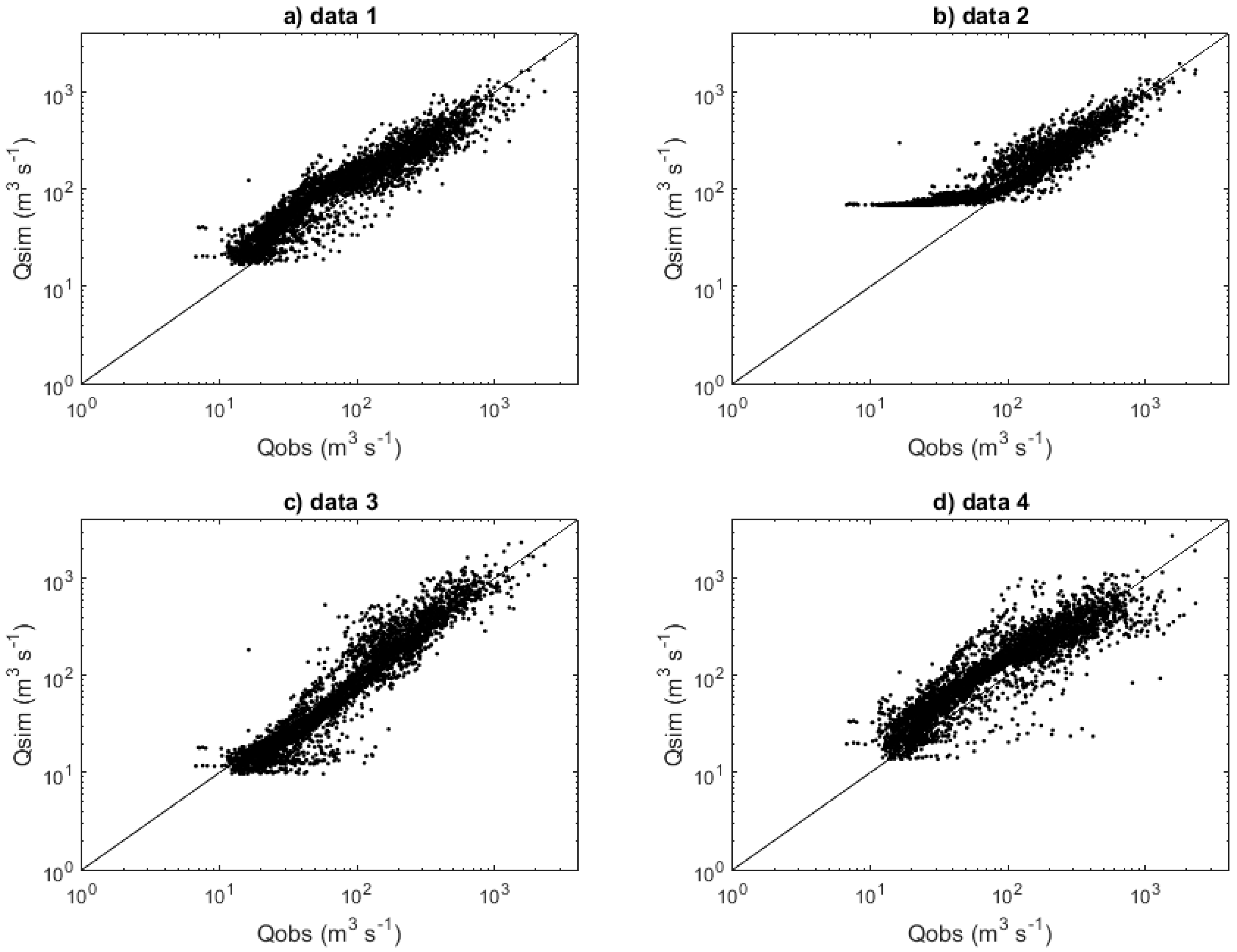
3.2. Calibration and Validation of the Hydrological Model

In the following step, hydrological model GR4J was calibrated (over the 1987–1993 period) and validated (over the 1995–2000 period) with the four meteorological data sets.

Table 3. Nash Sutcliffe Efficiency Coefficient (NS), Mean Absolute Percentage Error (MAPE) and Threshold statistics (TS) obtained in the calibration (Cal; 1987–1993) and validation (Val; 1995–2000) periods.

		Data 1	Data 2	Data 3	Data 4
NS	Cal.	0.79	0.87	0.88	0.54
	Val.	0.84	0.85	0.58	0.52
MAPE (%)	Cal	46.4	101.8	28.8	44.5
	Val	56.5	113.1	33.8	84.6
TS5 (%)	Cal.	6.9	7.9	7.2	8.0
	Val.	6.5	5.4	12.9	3.2
TS25 (%)	Cal	32.4	34.3	42.4	33.6
	Val	29.8	27.6	58.6	19.8
TS50 (%)	Cal	60.6	50	91.4	61.3
	Val	52.6	40.3	81.3	37.6

shows the performance of the hydrological simulations with several statistics: 1) the Nash Sutcliffe Efficiency Coefficient (NS) [33] which ranges from −∞ to 1, where 1 indicates a perfect match between simulated and observed discharge; 2) the Mean Absolute Percentage Error (MAPE) [34,35]; and 3) the Threshold statistics (TS), which is the number of data points with an absolute relative error less than x% [36]. A smaller MAPE and larger TS indicate a good performance.

From this table, it can be noted that the model calibrated and validated with data 1 (station observations) and with data 2 (a processed data set) obtains a good performance with NS values of 0.84 and 0.85 in validation period. Additionally, calibration with data 3 also achieves a good performance in calibration (0.88), but not in validation (0.58). In contrast, the hydrological model calibrated and validated through reanalysis data (data 4) presents the lowest performance, with NS values of about 0.54. The most important difference in NS values between calibration and validation periods is observed for data 3, as a result of variations in the precipitation annual cycle. For instance, in the wet season (May–October), the difference in precipitation is −194 mm for data 3, which is important compared with data 1, data 2, and data 4 (−18 mm, −50 mm and −67 mm, respectively). Furthermore, data 4 shows the precipitation peak in different months: July and August for the calibration and validation periods respectively. These results show mixed performance of the hydrological model in the simulation of the observed daily discharge in terms of the NS Efficiency Coefficient.

Further insight into the simulated discharges is shown in Figure 5, which presents the scatterplot of observed and simulated daily discharges obtained through the study meteorological data sets. This figure shows a good agreement between data 1 and data 3, with a slight overestimation and underestimation of medium flows respectively. In contrast, data 2 (Figure 5b) does not allow for simulation of low discharges and data 4 shows a large dispersion of the high flow scatters. The good performance of data 1 and data 2 in terms of NS is due to the importance of high flows as the NS coefficient is computed with differences between simulated and observed discharge as squared values [37]. Furthermore, data 2 shows a poor performance in terms of MAPE because this statistic yields to large percentage errors if the observed values are very small as in the case of low flows [35]. In contrast, data 3 shows a good performance in terms of MAPE and TS because of the good simulation of low and medium flows.

The four calibrated parameters of the conceptual model GR4J have no physical meaning; however, the study of Pagano et al. [38] assumed that each parameter of GR4J controls a process in the model: higher values of X1 (maximum capacity of the production store) increase soil moisture in the basin; X2 describes the exchange of water, whose value can be either positive (in case of water imports) or negative (for water exports; [31]); X3 (one day ahead maximum capacity of the routing store) controls the discharge of base flow, and X4 is the time base of the unit hydrograph, thus, higher values of this parameter attenuate the hydrograph. Analysis of the parameters shows that, when using data 1, GR4J considers that the soil moisture high (X1 = 1464 mm) and the water export positive (X2 = 1.8 mm). Regarding the behavior of the basin with gridded processed data, GR4J estimates a lower soil moisture in the basin (X1 = 164.6 mm and 49.3 mm for data 2 and data 3, respectively); moreover, the hydrological model assesses water imports for data 2 (X2 = 4.94 mm) and water exports for data 3 (X2 = −2.1 mm). In the case of reanalysis data (data 4), GR4J evaluates high moisture in the basin (X1 = 2957 mm) and water export (X2 = −5.1 mm). These results show that the selected datasets used to calibrate a lumped hydrological model result in four different representations of the study basin. The different representations of the basin’s hydrological system will be evaluated in the context of climate change.

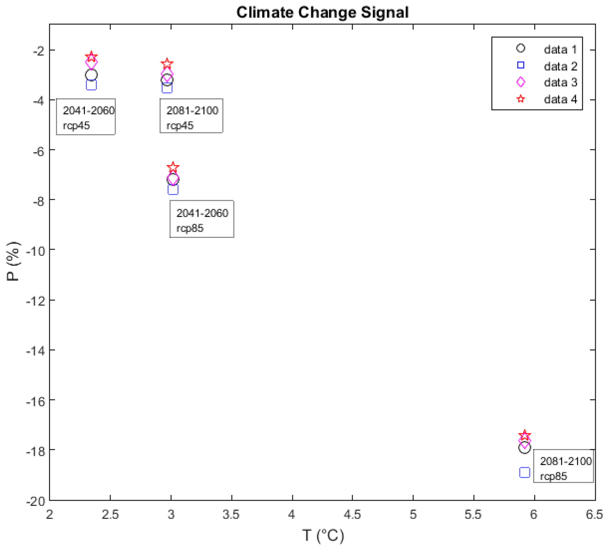
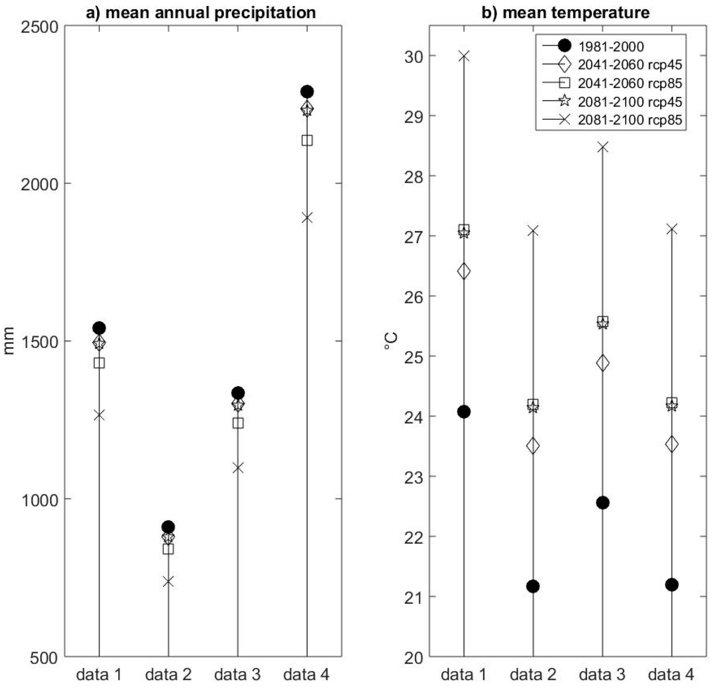
3.3. Climate Change Signal on Meteorological Variables

As mentioned before, each meteorological data set was used as a reference source in the bias corrected procedure. Figure 6 shows the mean climate change signal (computed with the five-member ensemble) for bias-corrected meteorological variables. Results show that the climate change signal (CCS) is similar among datasets for a given period and RCP. For instance, in the case of the 2041–2060 period and RCP 4.5 (rcp45 in Figure 6), the CCS in precipitation ranges from −2.3% to −3% and the change in temperature is about 2.3 °C. The largest change is estimated for 2081-2100 RCP 8.5 (rcp85 in Figure 6); thus, the CCS in precipitation ranges from −17.5% to −18.9%, while the CCS on temperature is about 5.9 °C. The bias correction procedure may change the climate change signal [39] so it can be noted that, for a given period and RCP, the evaluated change in precipitation varies slightly in accordance to the reference data set used.

Despite the similarities in terms of relative change, the absolute values of the future bias-corrected meteorological variables vary with the meteorological data set considered in the DT method. Figure 7 shows the five-member ensemble mean annual precipitation and temperature over the study basin for the RCPs and periods considered. From this figure, it can be seen that the lowest bias-corrected future precipitation is evaluated with data 2, while the highest is estimated with data 4, as in the historic period (Figure 3a). For example, the precipitation for RCP 85 2041–2060 ranges between data sets from 842 (data 2) to 2136 mm yr⁻¹(data 4), while for the same scenario in 2081–2100 precipitation ranges from 739 (data 2) to 1890 mm yr⁻¹(data 4). Similarly, the change in the bias-corrected temperature depends on the source of meteorological data set used, so for RCP 85 2041–2060 the temperature ranges from 23.5 °C (data 2) to 26.4 °C (data 1), while for the same scenario in 2081–2100, the temperature ranges from 27 °C (data 2) to 30 °C (data 1). These results show the effect of meteorological data set on statistical bias correction, based on the main hypothesis of time invariance of the bias, that is, that the bias in the historical reference period will be the same in future periods [40,41,42].

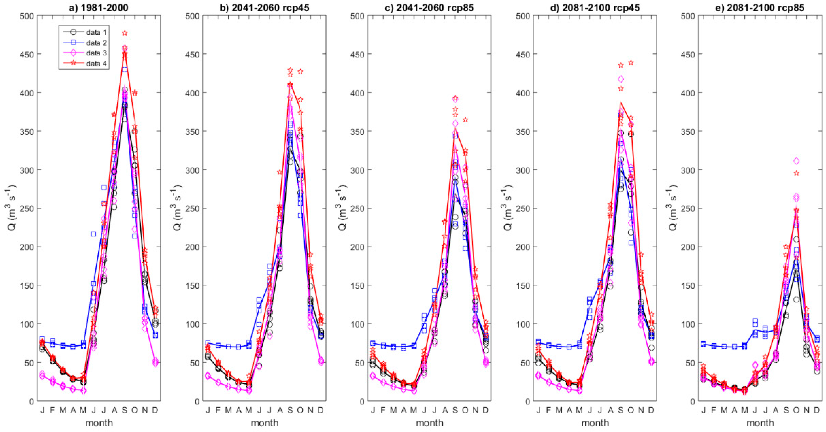
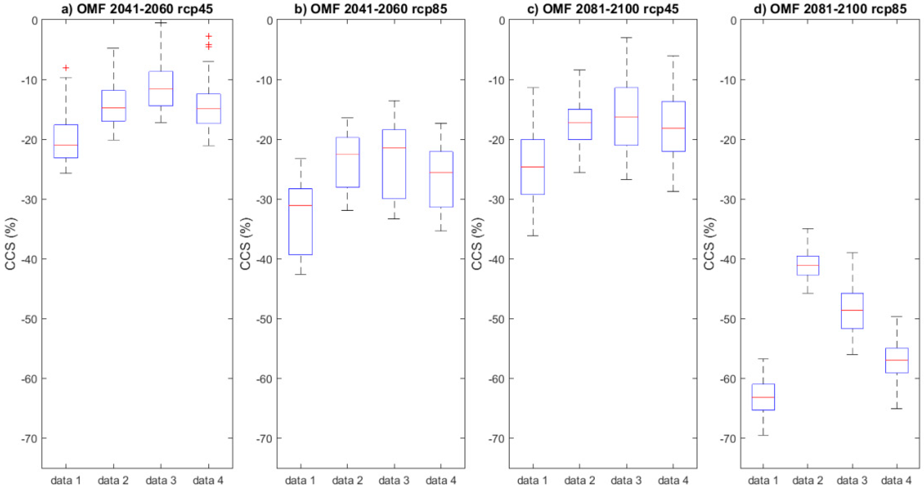
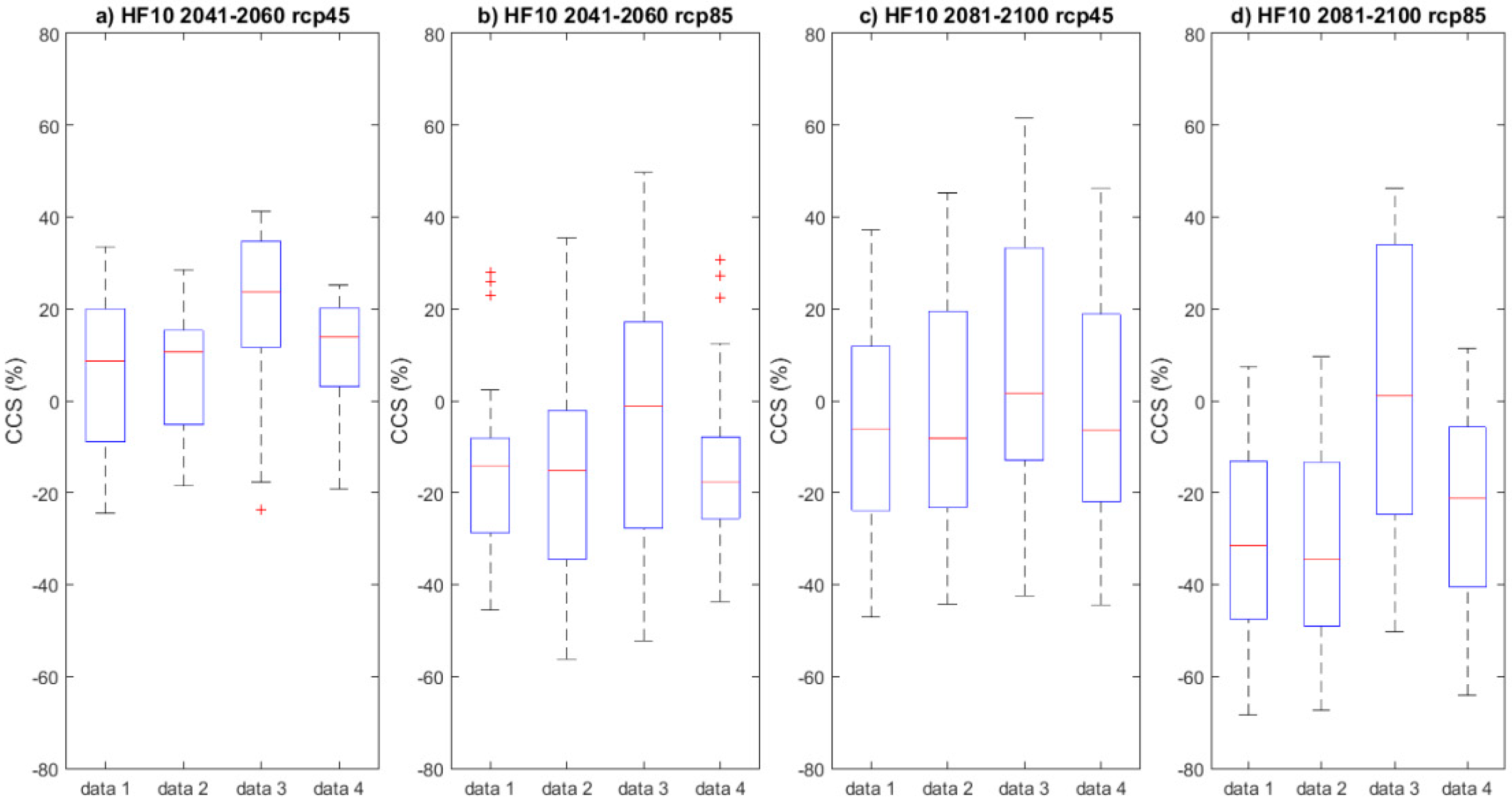
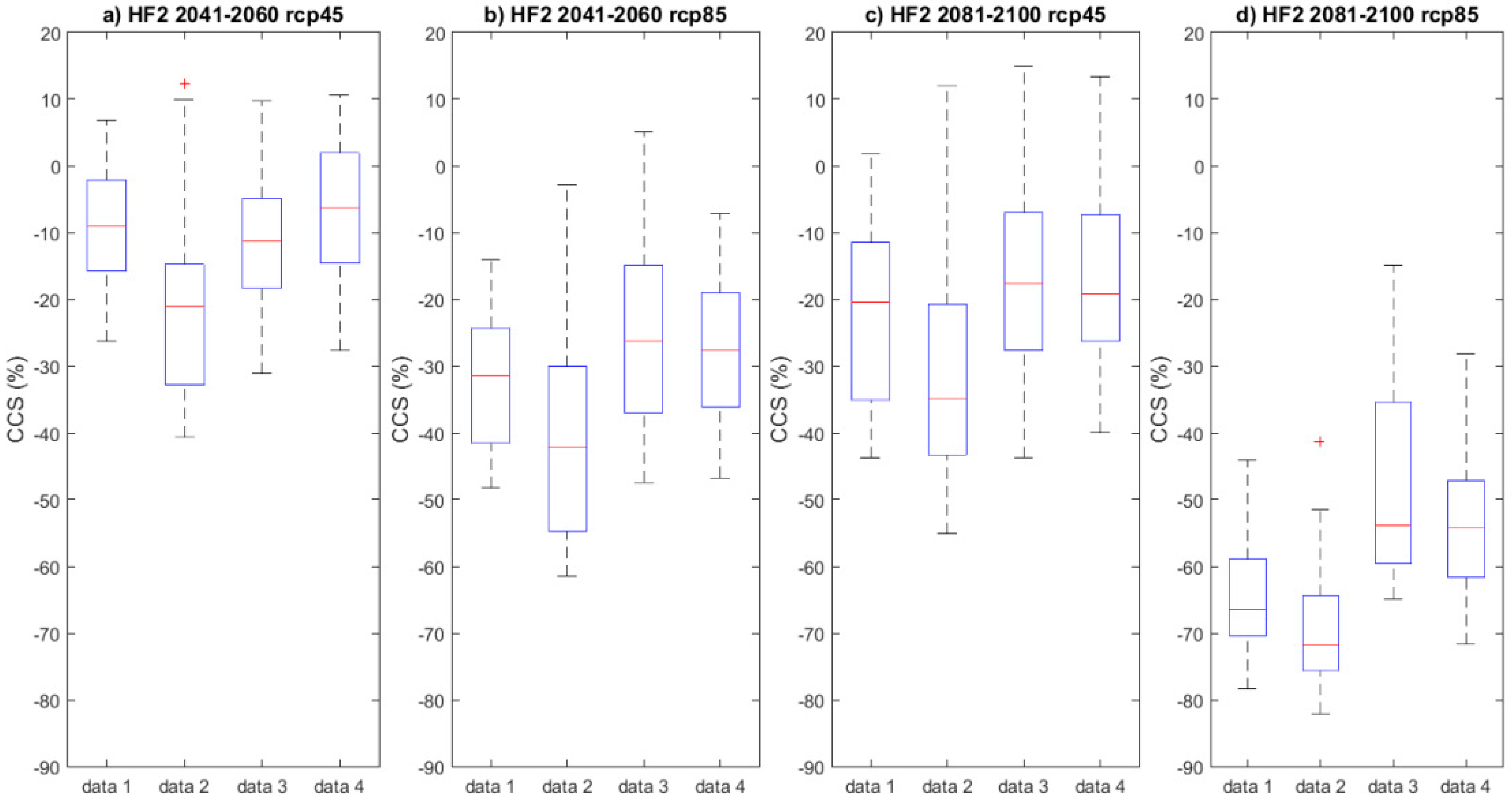
3.4. Climate Change Signal on Hydrological Indicators

In the following step, the calibrated hydrological model was fed with bias-corrected ensemble climate simulations. Figure 8 shows the mean monthly discharge in reference and future periods as computed with the hydrological simulations. For the reference period (Figure 8a), the September peak is simulated with all the meteorological data sets, with mean discharge values from 383 m³ s⁻¹ to 456 m³ s⁻¹. In this figure, the variability in the hydrological simulations as a result of the use of the ensemble of climate simulations can be noted. For example, in October, the discharge ranges from 213 m³ s⁻¹ to 277 m³ s⁻¹ with data 2, and from 222 m³ s⁻¹ to 296 m³ s⁻¹ with data 3; that is, the discharge values overlap between meteorological datasets. On the other hand, variability in the dry months is low. Figure 8a also shows that higher values of low flows in the dry season were obtained with data 2, as observed in the calibration and validation procedure (Figure 5b).

Regarding hydrological simulations 2041–2060 RCP45 (Figure 8b), the change in the September mean discharge (as compared with reference period) ranges from −19 m³ s⁻¹ (data 3) to −56 m³ s⁻¹ (data 1). The largest change in the September peak flow is evaluated in the horizon 2081-2100 RCP85 (Figure 8e), with values ranging from −252 m³ s⁻¹ (data 3) to −279 m³ s⁻¹ (data 4).

Figure 9 shows the climate change signal on the OMF indicator as evaluated with each meteorological data set. The methodology used to evaluate the CCS (see Equation (5)) allows comparison of the uncertainty related to the meteorological data set to the uncertainty related to natural variability, which is expressed in the spread of the relative changes on the hydrological indicators. The median changes in the OMF for the 2041–2060 period range from −11.6% to −20.9% for RCP 4.5, and from −21.5% to −31% for RCP 8.5, respectively (Figure 9a,b). Moreover, the median CCS evaluated with data 1 stands out with the highest CCS in all cases, especially for the 2081–2100 period RCP 8.5 (Figure 9d): the CCS median value for data 1 is −63.2%, while the CCS median value ranges from −41% to −56.9% with the other datasets; additionally, this example shows that uncertainty related to the dataset implemented is higher than uncertainty associated with the natural variability of climate simulations. In contrast, in the 2041–2060 period (Figure 9a,b) data 2, data 3, and data 4 the CCS more closely resemble data 1.

The CCS in HF2 is depicted in Figure 10. From this figure, it can be seen that the lowest CCS is evaluated in period 2041–2060 RCP 4.5 (median value from −6.2 to −21.1%, Figure 10a) and the highest CCS is evaluated in 2081–2100 RCP 8.5 (the median value ranges from −53.8% to −71.8%, Figure 10d). For this indicator, the most important change in the median CCS is estimated with data 2. For HF10 (Figure 11) the spread of the CCS is outstanding in period 2081–2100 RCP 45 (Figure 11c), ranging from about −40% to +60% for data 3, which covers the spread of the other boxplots.

In a subsequent step, a statistical test was performed in order to assess if the CCS from two datasets could be considered as issued from the same distribution, in order to use either of these meteorological datasets in the evaluation of the climate change impact on hydrological indicators.

The Wilcoxon test [43] (as computed with Matlab) evaluates if two samples of CCS, obtained from two different meteorological datasets, are independent samples from identical continuous distributions with equal medians (the null hypothesis).

Table 4. Results of Wilcoxon test comparing pairs of CCS. The p-value is shown and the shaded area indicates no rejection of the null hypothesis at significance level of 5%.

			Data 1–Data 2	Data 1–Data 3	Data 1–Data 4	Data 2–Data 3	Data 2–Data 4	Data 3–Data 4
OMF	2041–2060	rcp45	<0.001	<0.001	<0.001	0.017	0.815	0.017
		rcp85	<0.001	<0.001	<0.001	0.922	0.074	0.107
	2081–2100	rcp45	<0.001	<0.001	0.001	0.627	0.876	0.415
		rcp85	<0.001	<0.001	<0.001	<0.001	<0.001	<0.001
HF2	2041–2060	rcp45	<0.001	0.404	0.332	0.0041	<0.001	0.103
		rcp85	0.0137	0.107	0.187	0.001	0.0014	0.741
	2081–2100	rcp45	0.0379	0.341	0.180	0.0043	0.0019	0.800
		rcp85	0.0416	<0.001	0.0011	<0.001	<0.001	0.268
HF10	2041–2060	rcp45	0.907	0.0088	0.712	0.0043	0.404	0.013
		rcp85	0.999	0.0397	0.953	0.0457	0.969	0.071
	2081–2100	rcp45	0.938	0.1744	0.831	0.1806	0.892	0.207
		rcp85	0.712	<0.001	0.332	<0.001	0.193	0.001

presents the Wilcoxon test results showing the rejection (or not) of the null hypothesis at a 5% significance level.

Table 4 shows the results of the CSS pairs comparison. From this table, it can be seen that, for OMF, the null hypothesis is rejected in all periods and RCPs when the CCS obtained with data 1 (station data) is compared with the CCS obtained with the other datasets. However, the pair comparisons with data 2, data 3, and data 4 obtain no rejection for the null hypothesis in several cases when considering 2041–2060 RCP 8.5 and 2081–2100 RCP 4.5. On the other hand, the null hypothesis is rejected for all comparisons in 2081–2100 RCP 8.5.

For HF2, pairs comparing CCS from data 1 with data 3 and data 4 do not reject the null hypothesis, except for 2081-2100 RCP 8.5. For HF10, Table 4 shows that in the comparison between data pairs 1–2, 1–4, and 2–4, the null hypothesis is not rejected. The case of HF10 2081–2100 RCP 4.5 is outstanding, as the null hypothesis is not rejected with any pair combination.

These results show that for OMF, the CCS obtained from processed gridded data and the reanalysis is different from the CCS obtained through station data. Results are mixed for high flows, thus, the CCS obtained with station data is comparable with some of the selected datasets.

4. Discussion

In Mexico, as in other countries, historical meteorological data present issues (such as a low density of gauging stations or missing data) that hinder their use in hydrological modeling. In that respect, the interpolated meteorological and reanalysis data could be an alternative source of data to feed a hydrological model to simulate basin hydrology.

This study evaluates the uncertainty related to the choice of the meteorological data source; firstly, in the calibration and validation of a hydrological model; secondly, in the bias correction of climate simulations; and finally, in the evaluation of the impact of climate change on the hydrological indicators. In particular, four data sources were considered: observations, two gridded interpolated data sets, and one reanalysis data set.

The evaluation of the meteorological data shows that the interpolated datasets underestimate precipitation while reanalysis overestimates the observed precipitation. Regarding temperature, all datasets underestimate the observations. However, our results show a good performance of daily streamflow with the selected lumped hydrological model (GR4J) with all data sets, except reanalysis data. Comparison of the optimized parameters of the hydrological model shows that GR4J leads to different hydrological responses of the basin.

Bias correction of climate simulations was performed using each meteorological data set as proxy for the historical period. Results show that, for a given RCP and horizon, the relative change signal (i.e., in percentage) on precipitation and change in temperature is similar as it is conditioned by the difference between climate simulations in reference and future periods; however, the magnitude of future precipitation and temperature strongly varies due to differences between meteorological data sets used in the bias correction procedure.

Evaluation of climate change signal on hydrological indicators shows mixed results: in the case of overall mean flow, the uncertainty resulting from the meteorological source is greater than the uncertainty related to natural variability; thus, the use of interpolated and reanalysis data instead of observations leads to a different estimation of the climate change signal. On the other hand, the results in high flow indicators show that that climate change signals obtained from observations and the other data sources are comparable in several cases. Therefore, we must be cautious and evaluate the processed meteorological data sets before their use in the evaluation of climate change impact on water resources for the calibration of the hydrological model and as source data in the bias correction of climate simulations.

5. Conclusions

In this study, the uncertainty related to the choice of meteorological data was evaluated in the calibration and validation of a lumped hydrological model (GR4J), in the correction of climate simulations, and in the estimation of the climate change impact on hydrological indicators. Four datasets were evaluated: station observations, two gridded interpolated datasets, and reanalysis data. The main findings are:

• The meteorological data sets show underestimation (or overestimation in the case of the reanalysis) of precipitation and temperature. The hydrological model presents, to some extent, a good performance in terms of the Nash Sutcliffe Efficiency Coefficient. However, the analysis of the hydrological model’s optimized parameters shows important differences in their values, which indicates that the model leads to different representations of the basin’s hydrology.
• The use of the different meteorological data sets in the bias correction of climate simulations lead to a similar relative climate change signal (CCS, i.e., difference between reference and future period), but the magnitude of the estimated precipitation and temperature in the future periods strongly varies with the choice of dataset.
• The impact of climate change on hydrological indicators is influenced by the different model parameterization and the magnitude of the bias-corrected variables. The uncertainty related to the choice of the meteorological dataset was compared with the uncertainty related to the natural climate variability. Results show that, for the overall mean flow, the use of processed gridded data leads to a different estimation of the climate change signal. Results are mixed for the 2-year and 10-year return period high flow; thus, the CCS is, in some cases, similar to the CSS obtained with observations.
• The results on this work highlight that uncertainty related to meteorological data is not negligible when compared to natural climate variability; thus, the meteorological datasets should be evaluated before their use in the calibration of the hydrological model and in the bias correction of climate simulations for the estimation of the change impact. However, future work should consider other sources of uncertainty, such as the choice of general circulation model or regional model, the bias correction procedure, and the hydrological model.

References

1. Arnell, N.G.; Gosling, S.N. The impacts of climate change on river flow regimes at the global scale. J. Hydrol. 2013, 486, 351–364. [Google Scholar] [CrossRef]
2. Panagoulia, D. Impacts of GISS-modelled climate changes on catchment hydrology. Hydrol. Sci. J. 1992, 37, 141–163. [Google Scholar] [CrossRef]
3. Horton, P.; Schaefli, B.; Mezghani, A.; Hingray, B.; Musy, A. Assessment of climate-change impacts on alpine discharge regimes with climate model uncertainty. Hydrol. Process. 2006, 20, 2091–2109. [Google Scholar] [CrossRef]
4. Graham, L.P.; Hagemann, S.; Jaun, S.; Beniston, M. On interpreting hydrological change from regional climate models. Clim. Chang. 2007, 81, 97–122. [Google Scholar] [CrossRef]
5. Prudhomme, C.; Davies, H. Assessing uncertainties in climate change impact analyses on the river flow regimes in the UK. Part 2: Future climate. Clim. Chang. 2008, 93, 197–222. [Google Scholar] [CrossRef]
6. Velázquez, J.A.; Schmid, J.; Ricard, S.; Muerth, M.J.; Gauvin St-Denis, B.; Minville, M.; Chaumont, D.; Caya, D.; Ludwig, R.; Turcotte, R. An ensemble approach to assess hydrological models’ contribution to uncertainties in the analysis of climate change impact on water resources. Hydrol. Earth Syst. Sci. 2013, 17, 565–578. [Google Scholar] [CrossRef]
7. Troin, M.; Velázquez, J.A.; Caya, D.; Brissette, F. Comparing statistical post-processing of regional and global climate scenarios for hydrological impacts assessment: A case study of two Canadian catchments. J. Hydrol. 2015, 520, 268–288. [Google Scholar] [CrossRef]
8. Hydrological modeling of the Tampaon River in the context of climate change. Tecnología Ciencias Agua 2015, 6, 17–30.
9. Al-Safi, H.I.J.; Kazemi, H.; Sarukkalige, P.R. Comparative study of conceptual versus distributed hydrologic modelling to evaluate the impact of climate change on future runoff in unregulated catchments. J. Water Clim. Chang. 2019. [Google Scholar] [CrossRef]
10. Al-Safi, H.I.J.; Sarukkalige, P.R. Evaluation of the impacts of future hydrological changes on the sustainable water resources management of the Richmond River catchment. J. Water Clim. Chang. 2017, 9, 137–155. [Google Scholar] [CrossRef]
11. IPCC. Climate Change: Impacts, adaptation, and vulnerability. Part B: Regional aspects. In Contribution of Working Group II to the Fifth Assessment Report of the Intergovernmental Panel on Climate Change; Barros, V.R., Field, C.B., Dokken, D.J., Mastrandrea, M.D., Mach, K.J., Bilir, T.E., Chatterjee, M., Ebi, K.L., Estrada, Y.O., Genova, R.C., et al., Eds.; Cambridge University Press: Cambridge, UK; New York, NY, USA, 2014; p. 688. [Google Scholar]
12. Fekete, B.M.; Vörösmarty, C.J.; Roads, J.O.; Willmott, C.J. Uncertainties in precipitation and their impacts on runoff estimates. J. Clim. 2004, 17, 294–304. [Google Scholar] [CrossRef]
13. Biemans, H.; Hutjes, R.W.A.; Kabat, P.; Strengers, B.J.; Gerten, D.; Rost, S. Effects of precipitation uncertainty on discharge calculations for main river basins. J. Hydrometeorol. 2009, 10, 1011–1025. [Google Scholar] [CrossRef]
14. Getirana, A.C.V.; Espinoza, J.C.; Ronchail, J.; Rotunno-Filho, O.C. Assessment of different precipitation datasets and their impacts on the water balance of the Negro River basin. Hydrol. Process. 2010, 404, 304–322. [Google Scholar] [CrossRef]
15. Grusson, Y.; Anctil, F.; Sauvage, S.; Sánchez Pérez, J. Testing the SWAT model with gridded weather data of different spatial resolutions. Water 2017, 9, 54. [Google Scholar] [CrossRef]
16. Velázquez, J.A.; Dávila, R. Uncertainty related to processed gridded meteorological data: Implications for hydrological modelling. Ing. Investig. Tecnol. 2017, 18, 199–208. [Google Scholar] [CrossRef]
17. Gao, J.; Sheshukov, A.Y.; Yen, H.; Douglas-Mankin, K.R.; White, M.J.; Arnold, J.G. Uncertainty of hydrologic processes caused by bias-corrected CMIP5 climate change projections with alternative historical data sources. J. Hydrol. 2019, 568, 551–561. [Google Scholar] [CrossRef]
18. Peel, M.C.; Finlayson, B.L.; McMahon, T.A. Updated world map of the Köppen-Geiger climate classification. Hydrol. Earth Syst. Sci. 2007, 11, 1633–1644. [Google Scholar] [CrossRef]
19. Instituto Mexicano de Tecnología del Agua Banco Nacional de Datos de Aguas Superficiales (BANDAS). Available online: https://www.imta.gob.mx/bandas (accessed on 31 August 2019).
20. Livneh, B.; Bohn, T.J.; Pierce, D.W.; Muñoz-Arriola, F.; Nijssen, B.; Vose, R.; Brekke, L. A spatially comprehensive, hydrometeorological data set for Mexico, the USA, and Southern Canada 1950–2013. Sci. Data 2015, 2, 150042. [Google Scholar] [CrossRef]
21. Zhu, C.; Lettenmaier, D.P. Long-Term Climate and Derived Surface Hydrology and Energy Flux Data for Mexico: 1925–2004. J. Clim. 2007, 20, 1936–1946. [Google Scholar] [CrossRef]
22. Saha, S.; Moorthi, S.; Pan, H.-L.; Wu, X.; Wang, J.; Nadiga, S.; Tripp, P.; Kistler, R.; Woollen, J.; Behringer, D.; et al. The NCEP climate forecast system reanalysis. Bull. Am. Meteorol. Soc. 2010, 91, 1015–1057. [Google Scholar] [CrossRef]
23. CICESE Datos Climáticos Diarios del CLICOM del SMN. Available online: http://clicom-mex.cicese.mx (accessed on 31 August 2019).
24. NOOAA Spatially Comprehensive, Meteorological Data Set for Mexico, the U.S., and Southern Canada. Available online: https://data.nodc.noaa.gov/cgi-bin/iso?id=gov.noaa.nodc:0129374 (accessed on 31 August 2019).
25. Texas A&M University Website Global Weather Data for SWAT. Available online: https://globalweather.tamu.edu/ (accessed on 31 August 2019).
26. WMO. Guide to Hydrological Practices Volume I Hydrology—From Measurement to Hydrological Information WMO-No. 168; World Meteorological Organization (WMO): Geneva, Switzerland, 2009; p. 302. [Google Scholar]
27. Panagoulia, D. Hydrological modelling of a medium-size mountainous catchment from incomplete meteorological data. J. Hydrol. 1992, 137, 279–310. [Google Scholar] [CrossRef]
28. Arora, V.K.; Scinocca, J.F.; Boer, G.J.; Christian, J.R.; Denman, K.L.; Flato, G.M.; Kharin, V.V.; Lee, W.G.; Merryfield, W.J. Carbon emission limits required to satisfy future representative concentration pathways of greenhouse gases. Geophys. Res. Lett. 2011, 38, L05805. [Google Scholar] [CrossRef]
29. Braun, M.; Caya, D.; Frigon, A.; Slivitzky, M. Internal Variability of Canadian RCM’s Hydrological Variables at the Basin Scale in Quebec and Labrador. J. Hydrometeorol. 2012, 13, 443–462. [Google Scholar] [CrossRef]
30. Mpelasoka, F.S.; Chiew, F.H.S. Influence of rainfall Scenario Construction Methods on Runoff Projections. J. Hydrometeorol. 2009, 10, 1168–1183. [Google Scholar] [CrossRef]
31. Perrin, C.; Michel, C.; Andréassian, V. Improvement of a Parsimonious Model for Streamflow Simulation. J. Hydrol. 2003, 279, 275–289. [Google Scholar] [CrossRef]
32. Oudin, L.; Hervieu, F.; Michel, C.; Perrin, C.; Andreassian, V.; Anctil, F.; Loumagne, C. Which Potential Evapotranspiration Input for a Lumped Rainfall-Runoff Model? Part 2—Towards a Simple and Efficient Potential Evapotranspiration Model for Rainfall Runoff Modelling. J. Hydrol. 2005, 303, 290–306. [Google Scholar] [CrossRef]
33. Nash, J.E.; Sutcliffe, J.V. River flow forecasting through conceptual models, Part 1—A Discussion of Principles. J. Hydrol. 1970, 10, 282–290. [Google Scholar] [CrossRef]
34. Panagoulia, D.; Tsekouras, G.J.; Kousiouris, G. A multi-stage methodology for selecting input variables in ANN forecasting of river flows. Glob. Nest J. 2017, 19, 49–57. [Google Scholar] [Green Version]
35. Kim, S.; Kim, H. A new metric of absolute percentage error for intermittent demand forecasts. Int. J. Forecast. 2016, 32, 669–679. [Google Scholar] [CrossRef]
36. Zhang, D.; Ni, G.; Cong, Z.; Chen, T.; Zhang, T. Statistical interpretation of the daily variation of urban water consumption in Beijing, China. Hydrol. Sci. J. 2014, 59, 181–192. [Google Scholar] [CrossRef]
37. Legates, D.R.; McCabe, G.J., Jr. Evaluating the use of “goodness-of-fit” measures in hydrologic and hydroclimatic model validation. Water Resour. Res. 1999, 35, 233–241. [Google Scholar] [CrossRef]
38. Pagano, T.; Hapuarachchi, P.; Wang, Q.J. Continuous Rainfall-Runoff Model Comparison and Short-Term Daily Streamflow Forecast Skill Evaluation, Australia; CSIRO; Water for a Healthy Country National Research Flagship: Melbourne, Australia, 2010; p. 70. [Google Scholar]
39. Muerth, M.J.; Gauvin St-Denis, B.; Ricard, S.; Velázquez, J.A.; Schmid, J.; Minville, M.; Caya, D.; Chaumont, D.; Ludwig, R.; Turcotte, R. On the need for bias correction in regional climate scenarios to assess climate change impacts on river runoff. Hydrol. Earth Syst. Sci. 2013, 17, 1189–1204. [Google Scholar] [CrossRef] [Green Version]
40. Velázquez, J.A.; Troin, M.; Caya, D.; Brissette, F. Evaluating the Time-Invariance Hypothesis of Climate Model Bias Correction: Implications for Hydrological Impact Studies. J. Hydrometeorol. 2015, 16. [Google Scholar] [CrossRef]
41. Teutschbein, C.; Seibert, J. Is bias correction of regional climate model (RCM) simulations possible for non-stationary conditions? Hydrol. Earth Syst. Sci. 2013, 17, 5061–5077. [Google Scholar] [CrossRef] [Green Version]
42. Ho, C.K.; Stephenson, D.B.; Collins, M.; Ferro, C.A.T.; Brown, S.J. Calibration strategies: A source of additional uncertainty in climate change projections. Bull. Am. Meteorol. Soc. 2012, 93, 21–26. [Google Scholar] [CrossRef]
43. Wilcoxon, F. Individual Comparisons by Ranking Methods. Biom. Bull. 1945, 1, 80–83. [Google Scholar] [CrossRef]
Figure 1. Study basin.
Water 11 02110 g001
Figure 2. GR4J structure, adapted from Perrin et al. [31].
Water 11 02110 g002
Figure 3. Mean monthly precipitation (a) and temperature (b) for the Papagayo River Basin (1981–2000).
Water 11 02110 g003
Figure 4. Empirical cumulative distribution functions for daily precipitation (a) and mean daily temperature (b) for the Papagayo River Basin (1981–2000).
Water 11 02110 g004
Figure 5. Daily discharges as simulated with GR4J for the Papagayo River Basin for calibration (1987–1993) and validation (1995–2000) periods computed with the selected meteorological data sets.
Water 11 02110 g005
Figure 6. Mean climate change signal for bias-corrected precipitation and temperature.
Water 11 02110 g006
Figure 7. Five-member ensemble mean of bias-corrected annual precipitation (a) and temperature (b) over the study basin.
Water 11 02110 g007
Figure 8. Simulated mean monthly discharge in reference and future periods. The lines represent the mean of the five-member ensemble.
Water 11 02110 g008
Figure 9. Climate change signal as computed with Equation (5) for the Overall Mean Flow (OMF). The central mark in the boxplot is the median.
Water 11 02110 g009
Figure 10. Same as Figure 9, but for the 2-year return period high flow (HF2).
Water 11 02110 g010
Figure 11. Same as Figure 9, but for the 10-year return period high flow (HF10).
Water 11 02110 g011