1. Introduction
In recent times, numerous climate projection research works have predicted changes in the pattern and intensity of global precipitation by the end of the 21st century. The studies suggest an expected increase in rainfall in tropical regions and at high latitudes [
1], especially in the East Asian monsoon region [
2]. The sudden changes in rainfall patterns and intensity lead to water-related natural hazards, such as flooding, drought, rainfall-induced landslides and water-related epidemics. Of these hydro-meteorological hazards, flooding is considered to be the most recurrent and to have the highest risk [
3]. For this reason, there has been a world-wide endeavor in developing the efficient and accurate flood models which are crucial for flood disaster prevention and mitigation.
Over the past decades, numerous flood models have been developed that utilize different hydrological approaches. These hydrological model types can be classified as empirical (data driven), hydro-dynamic and physical process-based [
4]. The hydro-dynamic approach uses mathematical equations to replicate the fluid behavior, which are derived from applying physical laws to fluid motions. This technique can be grouped dimensionally into 1D, 2D and 3D models. The simplest illustration of a floodplain flow is to represent the flow as one-dimensional along the river channel. One-dimensional flood models simulate flows that are assumed to flow in a longitudinal direction, such as rivers and confined channels. These models are computationally efficient but are subjected to modeling limitations, such as the inability to simulate flood wave lateral diffusion, the subjectivity of cross-section location and orientation, and the discretization of topography as cross-sections rather than as a continuous surface [
4]. In this case, 2D models are used to simulate the floodplain flow, in order to visualize the extent of floods which 1D models cannot provide. Two-dimensional models simulate floods with the assumption that the water depth in a vertical direction can be neglected, in comparison to the other two dimensions. However, to allow the representation of vertical features, vertical turbulence, vortices and spiral flows [
4], 3D models are used. Three-dimensional models can also overcome the other limitations of 1D and 2D models, such as the inclusion of hydrostatic assumptions, viscous shear stresses, the bed friction of fluid components, etc. [
5]. However, 3D modeling is a fairly recent development and there are fewer studies regarding this compared to 1D and 2D models.
While 1D models are simpler and more preferred in practice, 2D models are more detailed and more reliable for complex flow simulations. However, 2D models are computationally heavy and data intensive, which can impose challenges for real-time flood forecasting [
6]. In order to overcome the long simulation times in 2D modeling, several techniques have been developed by some flood modelers. Some of these solutions are the adaptive mesh refinement (AMR) implementation in 2D modeling [
6,
7]. Another method is the hybrid 1D–2D variable grid sizing technique [
8].
The most recent approach is the combined 1D–2D method developed by the U.S. Army Corps of Engineers Hydrologic Engineering Center River Analysis System (HEC-RAS), which is one of the most widely used 1D river simulation models. The integrated approach allows the linkage between the 1D and 2D models and can dynamically represent the river and floodplain interactions [
9]. Since this update for the 1D–2D coupling simulation is quite recent, only a few researchers have tried this approach for flood simulation analysis [
10,
11,
12,
13]. Therefore, this study aims to assess the capability of the model technique in simulating a river levee break through a comparison with the observed results and simulated results from previously used 2D flood models, Gerris [
6] and Fluvial modelling engine (FLUMEN) [
14,
15]. Gerris is an open-source software that solves shallow water computations using the adaptive quadtree grid technique [
7], while FLUMEN (FLUvial Modelling Engine) solves the depth-averaged shallow water equations on unstructured adaptive meshes, which is used for modeling hydraulic complex situations [
16]. Some of the flood parameters explored and compared are the flood boundary extent, water level depth, change in inundation and flooded area, flow velocity and surface water elevation.
The structure of this paper is as follows:
Section 1 discusses the scientific problem, research background and the proposed solution, and
Section 2 provides a definition of the new flood modeling technique to be used in the simulation and the governing equations, as well as the numerical methods used.
Section 3 contains the domain description, data sources, pre-simulation conditions and methodology. The results and analysis are discussed in
Section 4, and finally, a summary and conclusion are provided in
Section 5.
3. Data and Methods
To test the efficiency of the technique developed in simulating flood inundation events, the data gathered from the 2002 Baeksan levee failure event in Nam river, Korea were used for validation. On the 10 August 2002, continuous torrential rainfall caused one of dams in the concrete embarkment of the Baeksan water purification plant to collapse, resulting in six villages being inundated by flood [
29]. Consequently, approximately 3.5 km
2 of agricultural land and 80 houses were flooded [
6], and 24 of those were completely destroyed. The negative effect of the event lead to further interest in developing efficient dam breach flood models. This event also provides reliable field data suitable for verification, which previous research has used for flood analysis [
6,
14,
15].
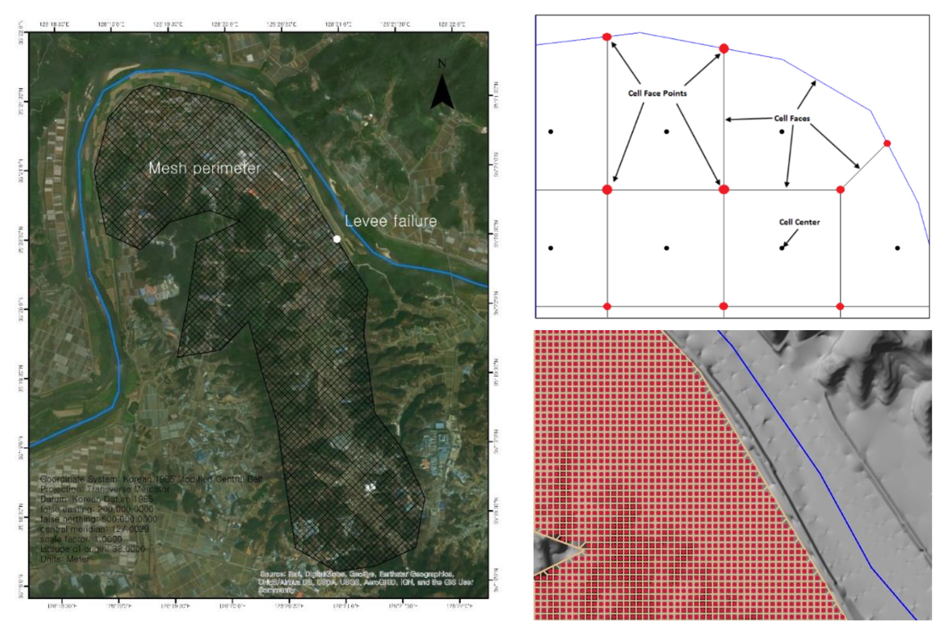
3.1. Research Domain
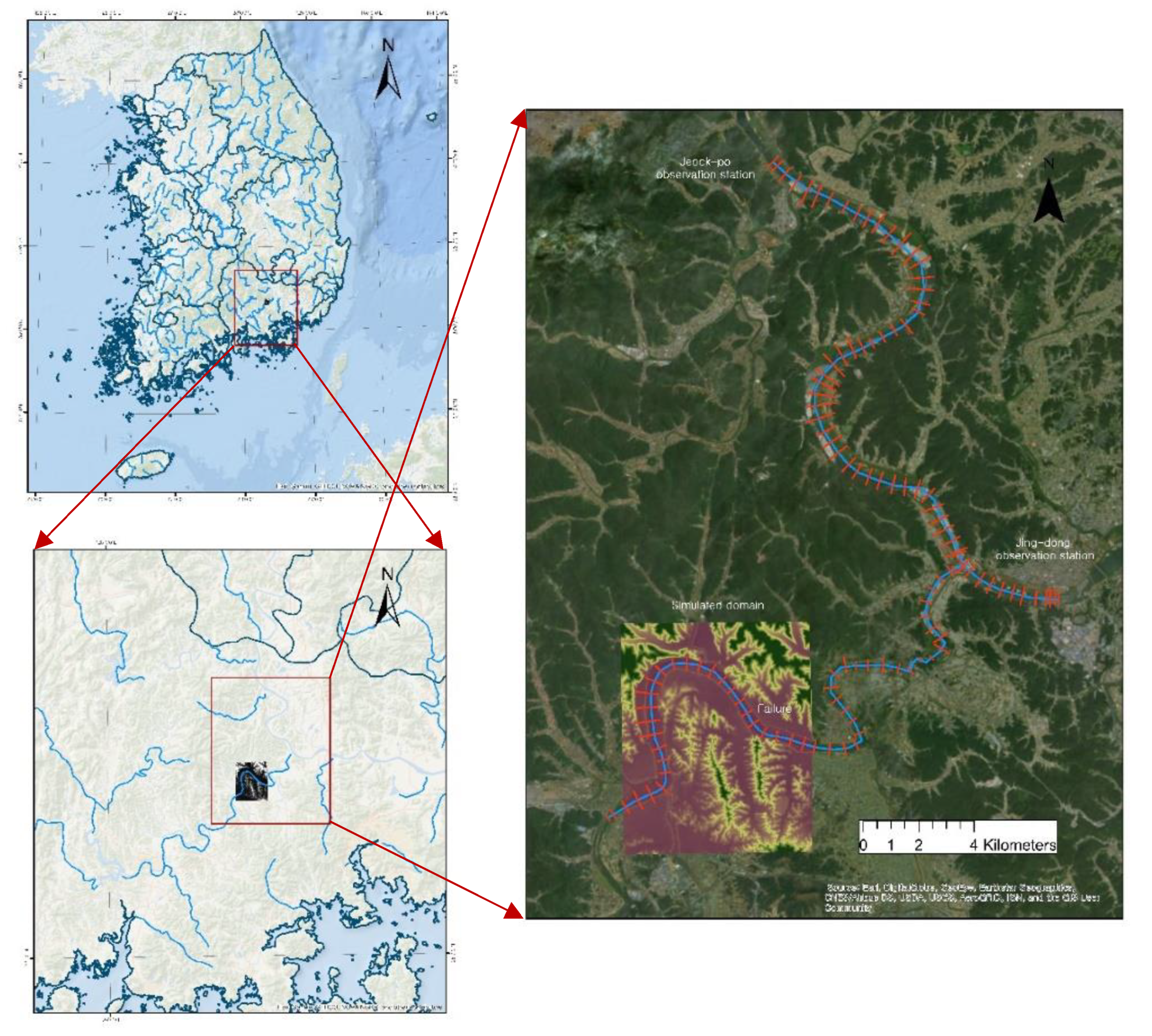
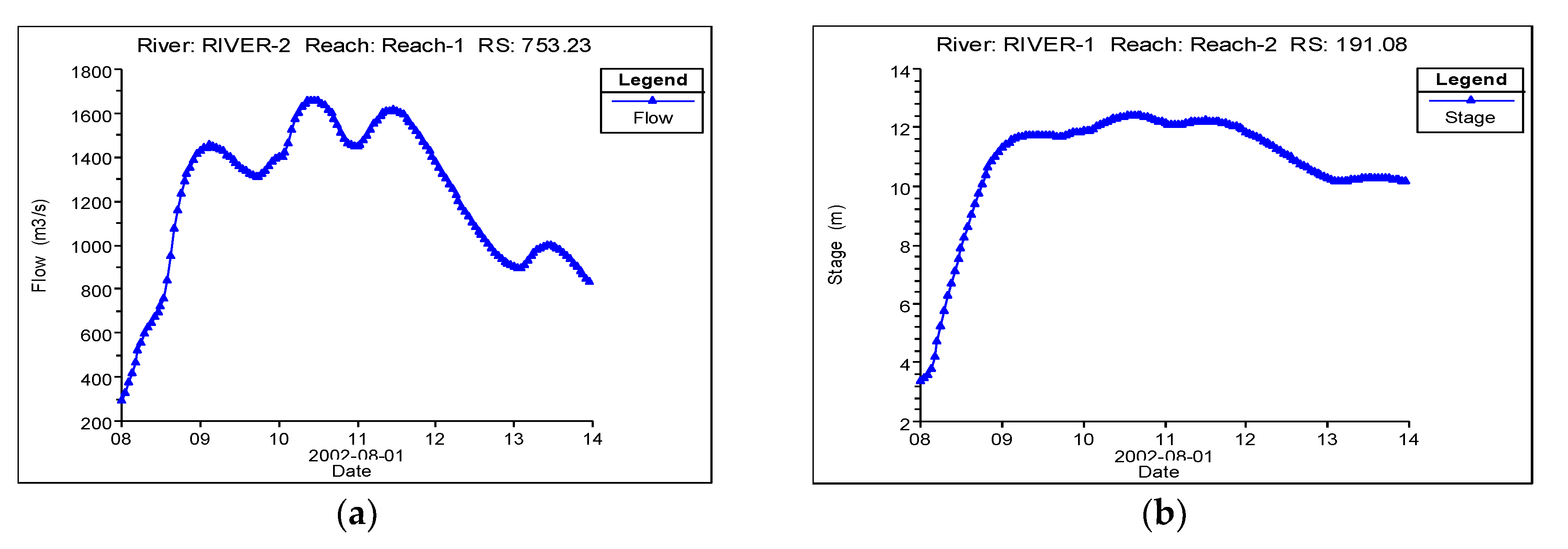
Figure 1 shows the geographical location of the study domain, the Baeksan–Nakdong river catchment. Nakdong river has three water level observation stations—Jeock-po, Jing-dong and Jeong-am stations—where the upstream and downstream boundary conditions used for this simulation were computed. The flow domain digital elevation model used for this research was provided by the National Geographic Information Institute of Korea. The flow rate and water level upstream and downstream boundary conditions (
Figure 2) used as input data were calculated using the HEC-RAS one-dimensional river routing model. The upstream boundary condition is a flow hydrograph of discharge over time, while the downstream boundary condition is a water surface elevation stage hydrograph versus time.
3.2. Methodology
In order to run the simulation for the HEC-RAS coupled 1D–2D model, the results from the HEC-RAS one-dimensional model were used for the input data. These 1D data were also used in previous research in simulating Baeksan flood inundation. The mesh domain for the 2D flow was set up, as well as the lateral structure and boundary conditions. After running the simulation, the resulting flood data—flood extent, water surface elevation, water depth, change in flooded area and flow velocity—were mapped using the geographic information system (GIS) tool, and then compared to the flood results from the observed data, Gerris and FLUMEN models. In this way, the model’s capability and accuracy can be assessed.
3.3. Pre-Simulation Conditions
In 2D modeling, a spatial representation of flow can either be constructed through a structured mesh (regular grid), unstructured mesh (triangular grid) or flexible mesh. However, difficulties in the simulation can be encountered in some cases where topographic data is too dense to be realistically used as a grid for numerical modelling. This poses challenges when a coarse grid must be used to generate an overall fluid simulation, but finer features needed to be incorporated in the computation as well. To solve this problem, recent advances in two-dimensional modeling include the adaptive mesh refinement method [
6] and hybrid 1D–2D variable grid sizing technique [
8]. HEC-RAS, however, uses the sub-grid bathymetry approach, where the extra information is pre-computed from fine bathymetry. The high-resolution details are neglected, but enough data are available so that the coarser numerical method can account for the fine bathymetry through mass conservation [
9]. Equation (4) requires knowledge on the sub-grid bathymetry, such as the cell volume
and face areas
as a function of water elevation
. The construction of the mesh in this simulation can be seen in
Figure 3. A hybrid discretization, as discussed in
Section 2.3, was used to tackle the challenge in discretizing orthogonal and un-orthogonal grids. In this research, a grid resolution of 33 by 33 m was used, conforming with the maximum level refinement criteria used by An et al. [
6].
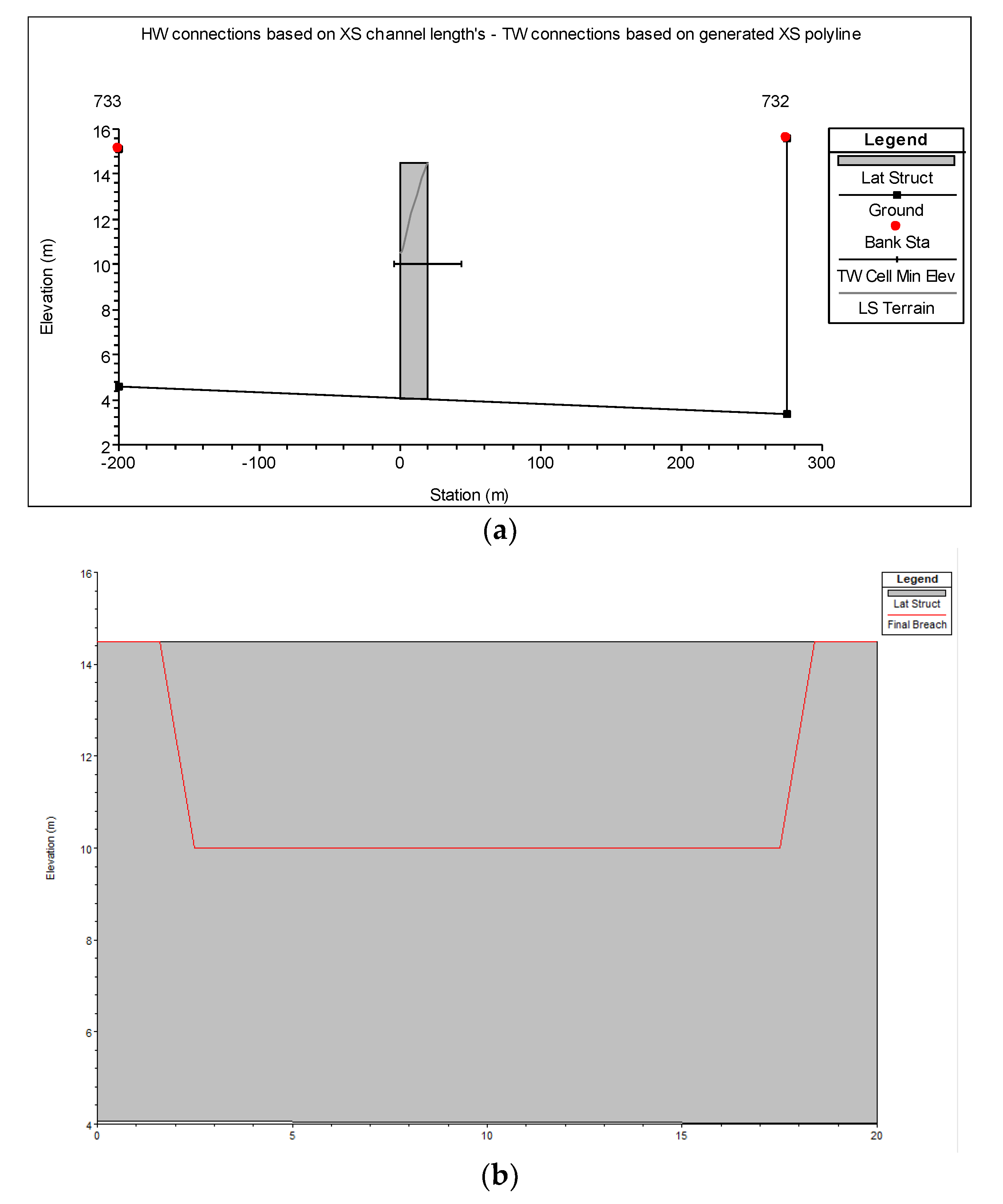
For the levee breach simulation, the upstream and downstream boundary conditions of water level and stage flow (
Figure 2) from the connecting water level observation stations were computed using the HEC-RAS 1D model. The lateral structure and the breach data of the ruptured levee can be seen in
Figure 4. The width and length of the failure were set as 10.3 m and 15 m, respectively, based on the survey conducted by the Korea Ministry of Construction and Transportation after the event. The homogeneous roughness coefficient is set to
according to the cultivated crop/pasture manning value in [
30], since the flood area is mostly paddy field and vegetable crops [
15].
The breach formation time was assumed to be 20 h, that is, the time it took for the surface water level in the flooded area side of the levee to recede after the breach. Our literature review stated that the levee break occurred on 10 August 2002 at 1600, and the flood simulation time was therefore set up for 10 August at midnight to 12 August at 1600. The simulation times for the FLUMEN, Gerris and HEC-RAS coupled 1D–2D were 420 [
29], 111.95 [
15] and 1.82 min, respectively.
4. Results and Analysis
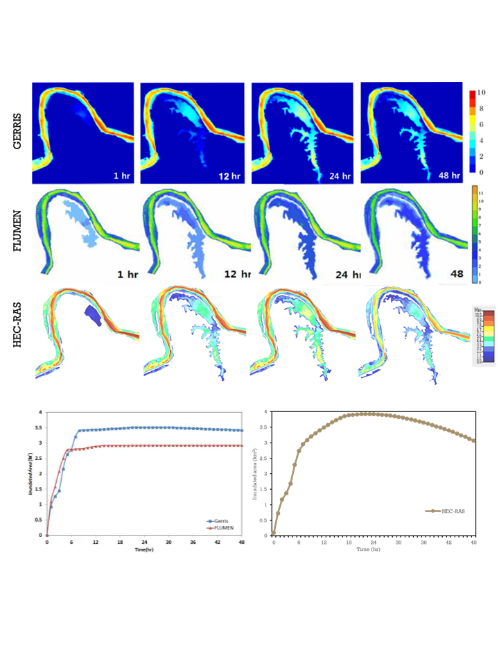
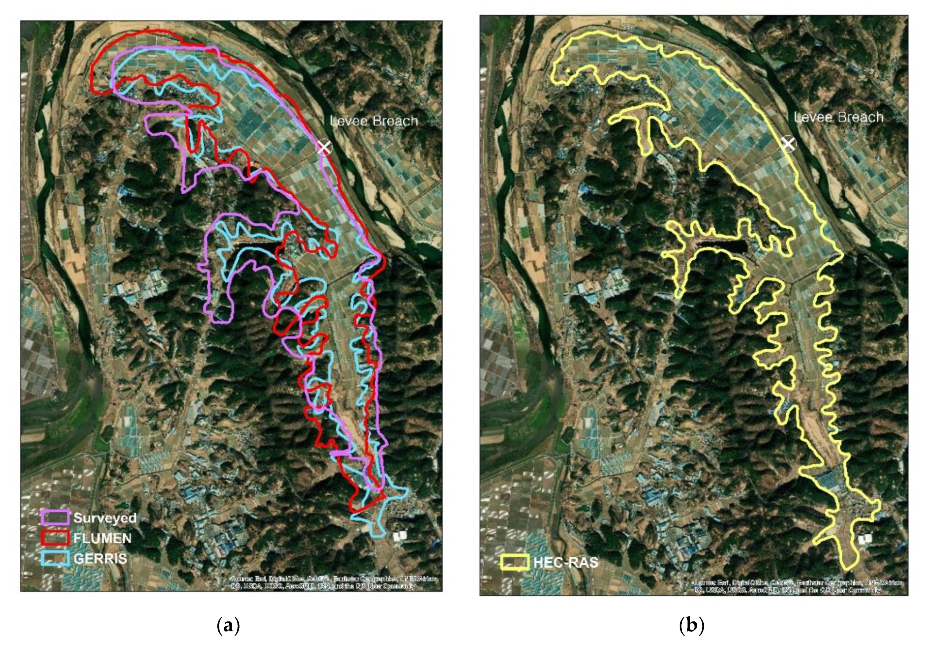
To analyze the performance of the HEC-RAS 1D–2D coupled method, the resulting flood simulations outputs were compared to those of the observed values (surveyed flood extent trace map by Korea Geongnam Development Institute, Busan, Korea) and the results from the 2D flood models (Gerris; FLUMEN) in previous research.
Figure 5 shows the surveyed flood inundation (red line) and simulated inundation boundaries (Gerris = purple line, FLUMEN = blue line, HEC-RAS = yellow line). In general, the flood extent simulated using HEC-RAS agrees well with the other models’ results and the surveyed one. The simulated inundation extents agree with the local topography. However, it under-estimated the expanse in comparison with the surveyed data, especially towards the mountainous areas. In terms of the maximum inundation area, HEC-RAS has a slightly greater value (3.88 km
2) compared to that of FLUMEN and Gerris (3.13 and 3.51 km
2, respectively).
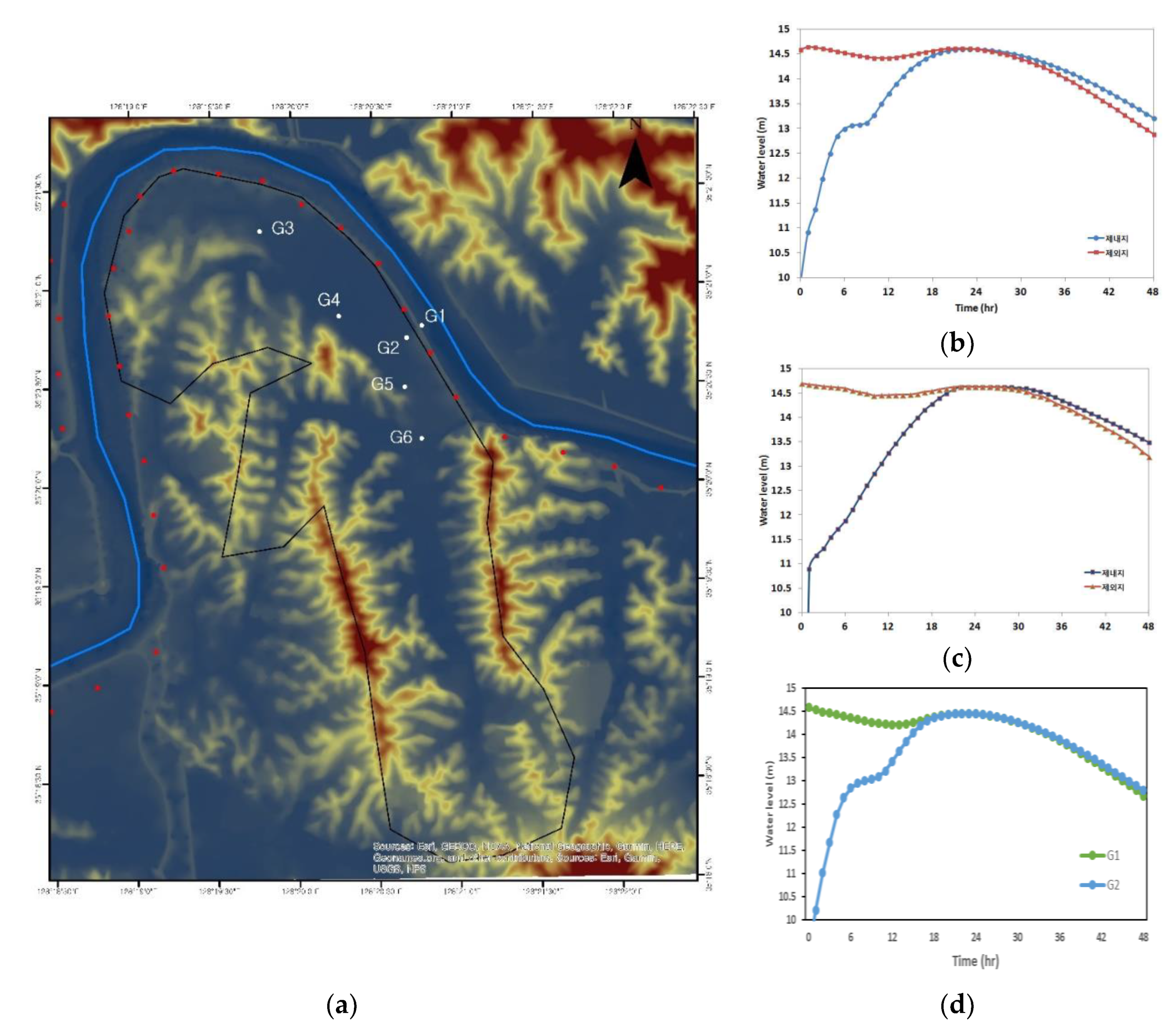
The flood points within the flooded area can be seen in
Figure 6. Points G1 and G2 are assigned on the river side and flooded area side of the levee, respectively. In this way, the simulated increase and decrease in the water level inside and outside the levee break can be visualized. The simulated change in water level on points G1 and G2 for the three models can be seen in
Figure 6. The simulation starts as the levee breaks on 10 August at 1600, and the water level in G1 slowly declines and the G2 water level sharply increases as water in the river flows into the paddy field. At around 22 h after the breach, the water level within the flooded area stabilizes and slowly drops as water starts to flow back into the river. The HEC-RAS simulated water level has the same pattern as that of the other two models, especially Gerris, where the water level is briefly stable around 6 to 9 h after the breach (13.0 m). The Gerris model reached 14.59 m at 24 h, while FLUMEN and HEC-RAS reached their maximum water levels at 22 h at 14.63 m and 14.45 m, respectively. In addition, in HEC-RAS, G1 and G2 water levels eventually even out as the water recedes, while for the other two models, the G2 water level is consistently higher than in G1. This might be due to the direct interaction of HEC-RAS 1D and 2D models, which allows the direct linkage of water flowing back into the river.
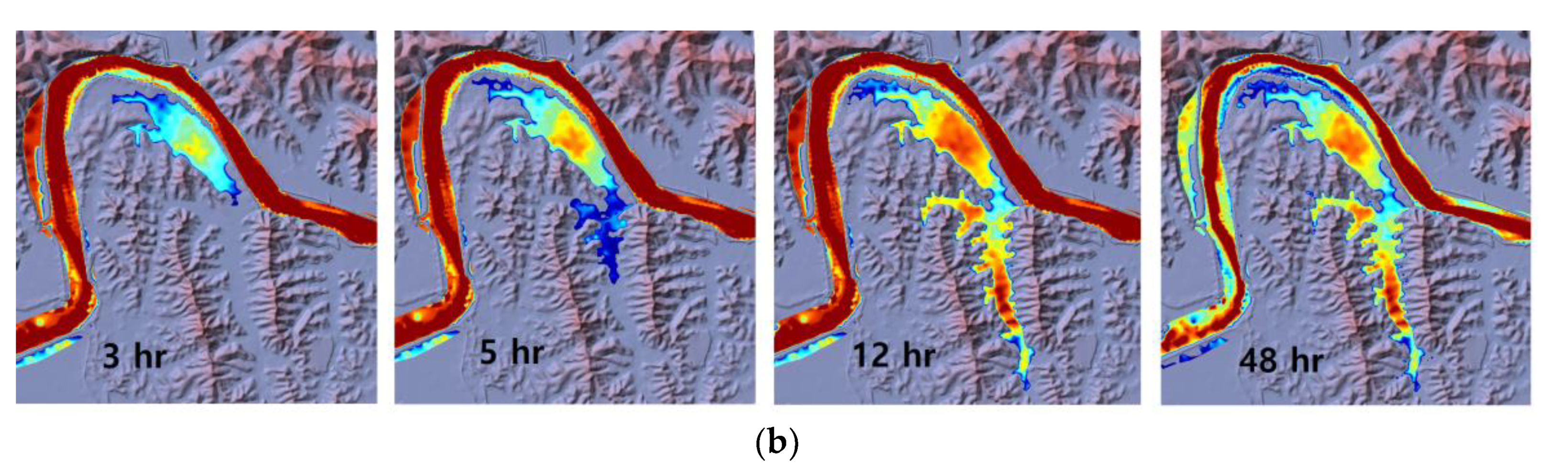
The simulated flood depth comparison of Gerris and HEC-RAS (
Figure 7) shows flood depths simulated by the two models 3, 5, 12 and 48 h after the levee break. The calculated water depth is the computed difference in the water surface elevation and surface elevation. The model outputs are quite similar, with minor differences in the depth and extent in some areas. Gerris has a wider and deeper flood inundation in time compared to HEC-RAS. Both models agree that the flood starts to recede back into the river after 48 h.
Both Gerris and HEC-RAS have the ability to simulate the flow velocity as well.
Figure 8 shows the simulated flow velocity comparison of the Gerris and HEC-RAS models. The water flows from the levee breach within the first to fifth hour and starts to recede after 48 h. The flow velocity is greatest within the levee opening and the sudden narrowing regions (
Figure 8).
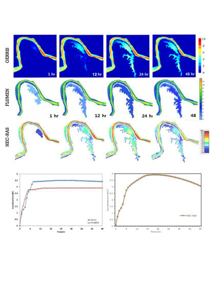
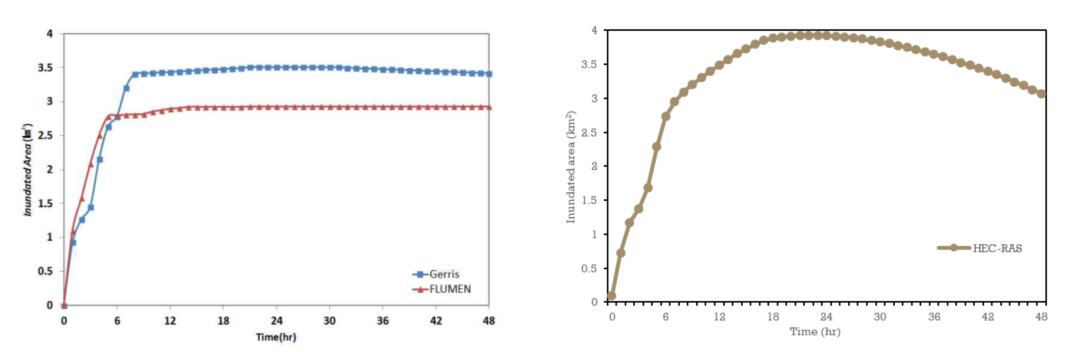
The change in the flooded area for the simulated results was calculated using GIS. A comparison between the models can be seen in
Figure 9. The results show an increasing flooded area for the three models. Gerris and FLUMEN show a similar trend: A constant increase in area from 0 to 5 h (95% flooded) (FLUMEN) and 0 to 8 h (97%) (Gerris). The estimated inundation was 2.8 km
2 for FLUMEN and 3.5 km
2 for Gerris, which remained constant until the end of the simulation. For HEC-RAS, however, an inconsistent increase in flooded area can be observed, where the maximum area simulated is 3.93 km
2 at 2200, and then this starts to decrease in size afterwards. The flooded area for HEC-RAS reached 75% after 7 h and 97% after 16 h. This behavior was not observed in the other two models. The reason for this might be because Gerris and FLUMEN model simulations considered the levee break as a topographical misalignment, in which the flow of water is only one way, while the HEC-RAS 1D–2D coupled method considers the interconnection between the 1D river flow and the 2D flood inundation. The recedence of water back into the river was considered in HEC-RAS, which is more realistic compared to the other models. Another reason may possibly be the difference in the threshold level for the three models. The models have different threshold values on which they count the wet and dry grid.
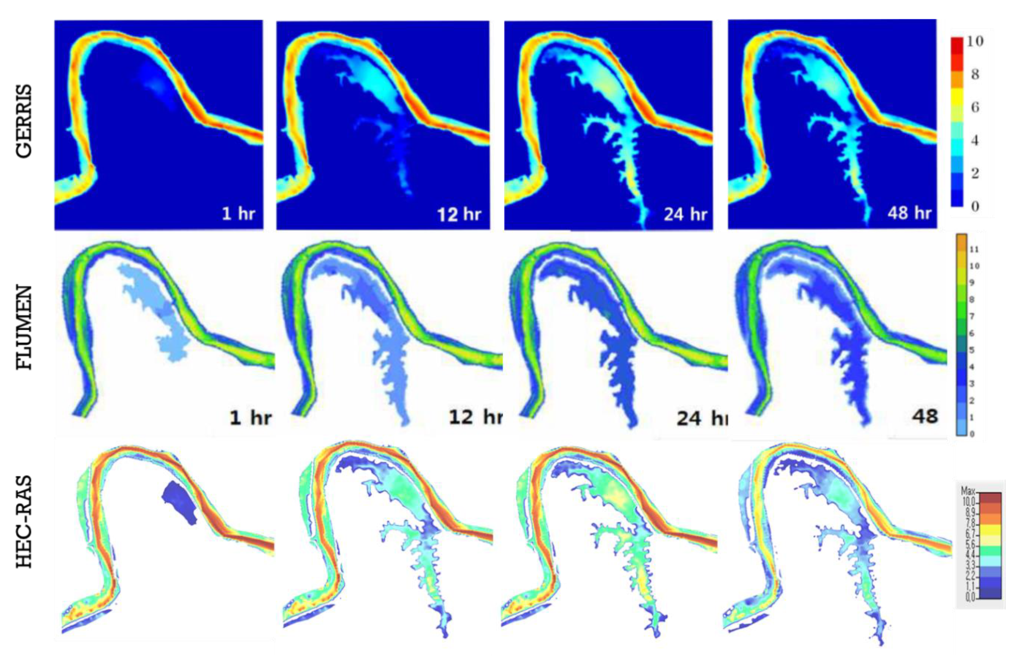
The surface water elevation values of Gerris, FLUMEN and HEC-RAS (
Figure 10) simulated at 1, 12, 24 and 48 h after the breach show similarities. FLUMEN at 1 h shows a slightly larger extent of inundation compared to the other two models. Lee et al. [
14] suggested that the difference might be due to the fact that the FLUMEN model considers the underflow flooding within the flooded area or due to the terrain differences. A slightly lower extent of the flood can be observed in the HEC-RAS model (
Figure 7 and
Figure 10) in the first five hours after the breach. This is because of the difference in the treatment in the overtopping process, where HEC-RAS utilizes a more detailed breaching procedure compared to the other models.
5. Conclusions
This research utilized the combined 1D–2D flood modeling capability of the HEC-RAS model to simulate the Baeksan levee break event in Korea in August 2002. The HEC-RAS coupled 1D–2D method used the sub-grid bathymetry approach and hybrid discretization to simulate the flood inundation. The accuracy of the simulation results was assessed by comparing them with the observed data, as well as the simulation results from other previously used 2D models, Gerris and FLUMEN. The flood results evaluated were the flood inundation boundary extent, water depth, flow velocity, surface water elevation and change in flooded area. These variables were represented as maps using GIS tools.
The flood simulation results from the HEC-RAS model show a large number of similarities to those of Gerris and FLUMEN models, with only some minor differences. A slight difference can be observed in the inundation extent in the first few hours after the breach in the HEC-RAS model, which is due to the more detailed breaching process of the model. A particular disparity was also observed in the change in flooded area over time. The resulting HEC-RAS model pattern in the change in flooded area shows an inconsistent increase in flooded area: 75% and 97% of the total flooded area are inundated 7 and 16 h after the levee breach, respectively, while Gerris and FLUMEN models achieved 95% and 97% of the inundated area 5 and 8 h after the breach, respectively. The dissimilarity in the results is possibly due to the difference in the numerical scheme and the treating approaches used by the models, and the direct connection between the 1D and 2D models in HEC-RAS, which allows direct feedback between the 1D and 2D flow elements occurring in the hydraulic link structure. The HEC-RAS simulated flooded area is deemed to be more realistic in terms of the ideal behavior of flood dynamics.
In conclusion, the ability of the latest HEC-RAS model to provide combined numerical computations of 1D river flow and 2D flood area has shown to be efficient in simulating levee breach events, which is of utmost importance, as flood events such as this are likely to occur with more frequency in the future.


