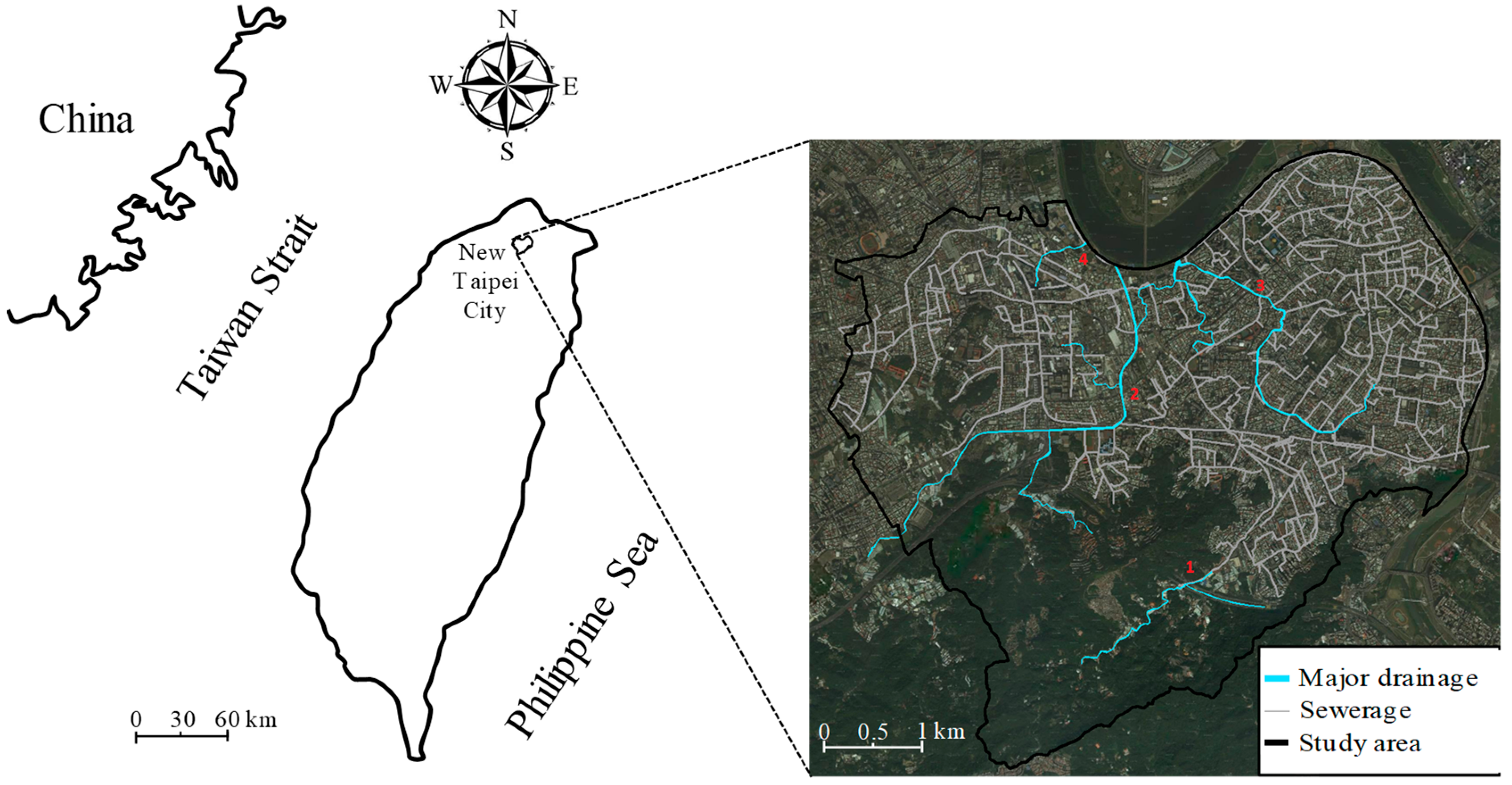
The parameters for the SWMM simulations were verified with inundated places in the study area. The SWMM was used for flow routing in storm sewers and the two-dimensional overland flow model was employed for the calculation of surface flooding [
20]. The inlets and junctions of the sewer systems were applied as the connecting points between SWMM and the two-dimensional overland flow model. The inlet was treated as the sink and the junctions were treated as source for this two-dimensional model. The detail of the interaction simulation between SWMM and two-dimensional overland flow model can be referred to in the previous study [
20]. The inundated places simulated in this study were compared to the surveyed data in two typhoon events (Typhoon Herb and Typhoon Nari). The accuracy was 96.3% and 89.5%; therefore the settings employed in SWMM were suitable for the LID simulation.
4.1. Influence of Different Rainfall Durations on LID and Detention Pond
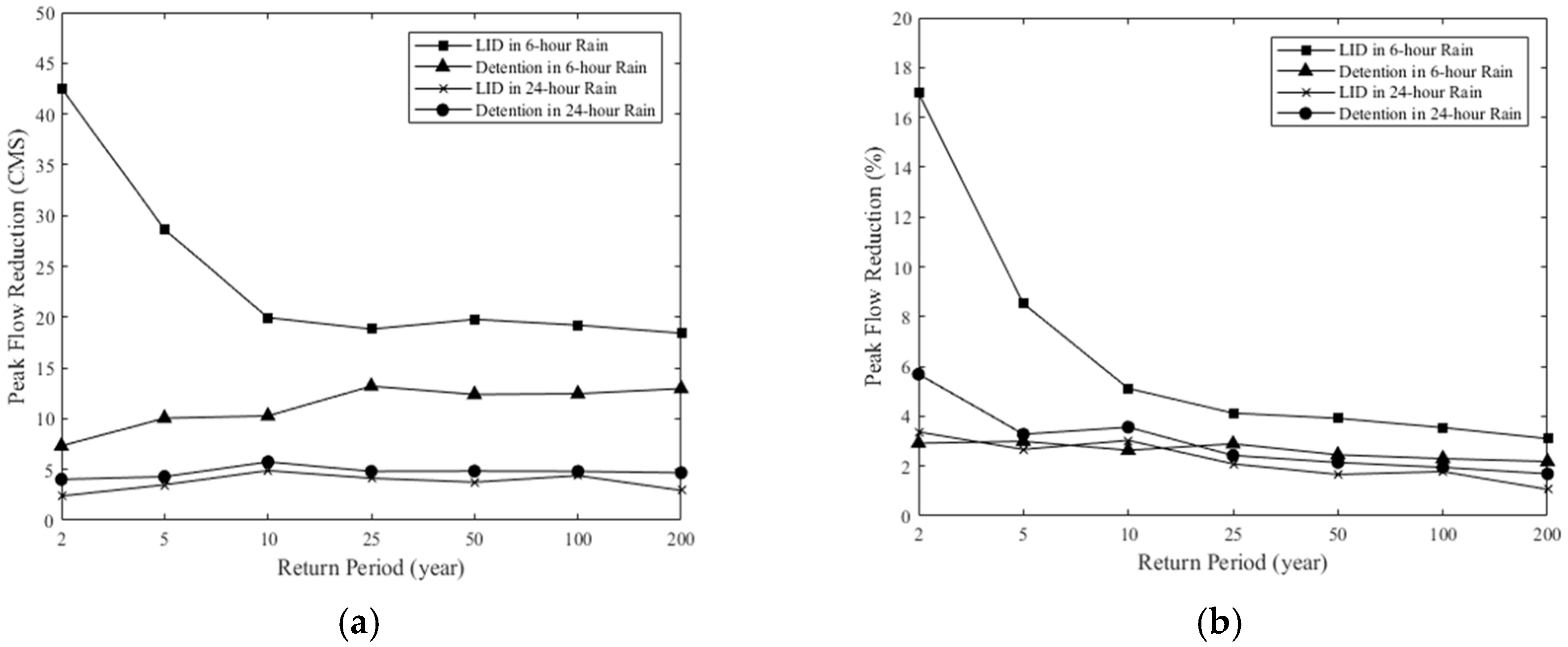
The performance of LIDs to reduce the flood peak and the HFR were investigated under 14 scenarios. For the six-hour duration case, the flood reduction by LIDs could reach the maximum volume for the two-year return period, and became constant after the 10-year return period. The reduction by detention ponds, on the other hand, could increase with the return periods (see
Figure 4a). This result told us that the detention pond could make up the disadvantage of the LID for large storm events, and the combination of them could be the proper strategy for the flood mitigation. Bai et al. [
21] also suggests that a proper design to combine LIDs and detention ponds might be the solution for storm management in the urban area. For the 24-hour duration case, the performance of LIDs to reduce the flood peak generally was poor when compared to the detention ponds. This showed that the capability of LIDs to reduce the floods was low for long durations. For the long duration and intensive rainfall cases, the detention ponds were more suitable than LIDs for flood reduction. The decreasing trend could be observed for the performance of LIDs to reduce the flood peak and the limitation was the 10-year return period for the six-hour duration case (see
Figure 4b). In terms of the 24-hour duration, the performance of the detention ponds kept the reduction rate at least 3% throughout all return periods. The above results demonstrated that LIDs can only reduce the flood peak effectively in the short duration and low intensity rainfall; moreover, they could play the advantage if the return period was less than 10 years. Pereira Souza et al. [
22] conduct a hydrological modeling for the performance of LID and show that the 10-year return period rainfall is the limitation for storm control in urban areas. The function of LIDs essentially was increasing infiltration and containing the runoff by increasing many small storage spaces. The infiltration rate would be reduced over time, and once the rainfall duration was long and reached the limitation of infiltration rate, the effect of LID units would be minimized. Therefore, if the vulnerability of cities is caused by the short duration with the low return period, LIDs should be first considered, otherwise detention ponds should be given the priority. Rezaei et al. [
23] also demonstrates that detention ponds are the proper solution to the flood control for long durations. In this study, the effect of detention ponds for flood reduction did not perform very well because those ponds were allocated in the existing parks and schools of the study area and these spaces were already designed at the end of the drainage system. In fact, the performance of the dentation ponds was highly affected by the location. If ponds were allocated at the downstream of the drainage system, the reduction rate would be less than at the upstream of the system. Those ponds were only allocated in the existing parks and schools since the study area was crowded and developed, and there was no available space for retrofitting. Even though the performance of detention ponds was not the best for this simulation, the trend of results showed that the detention ponds were superior than LIDs in the large return periods.
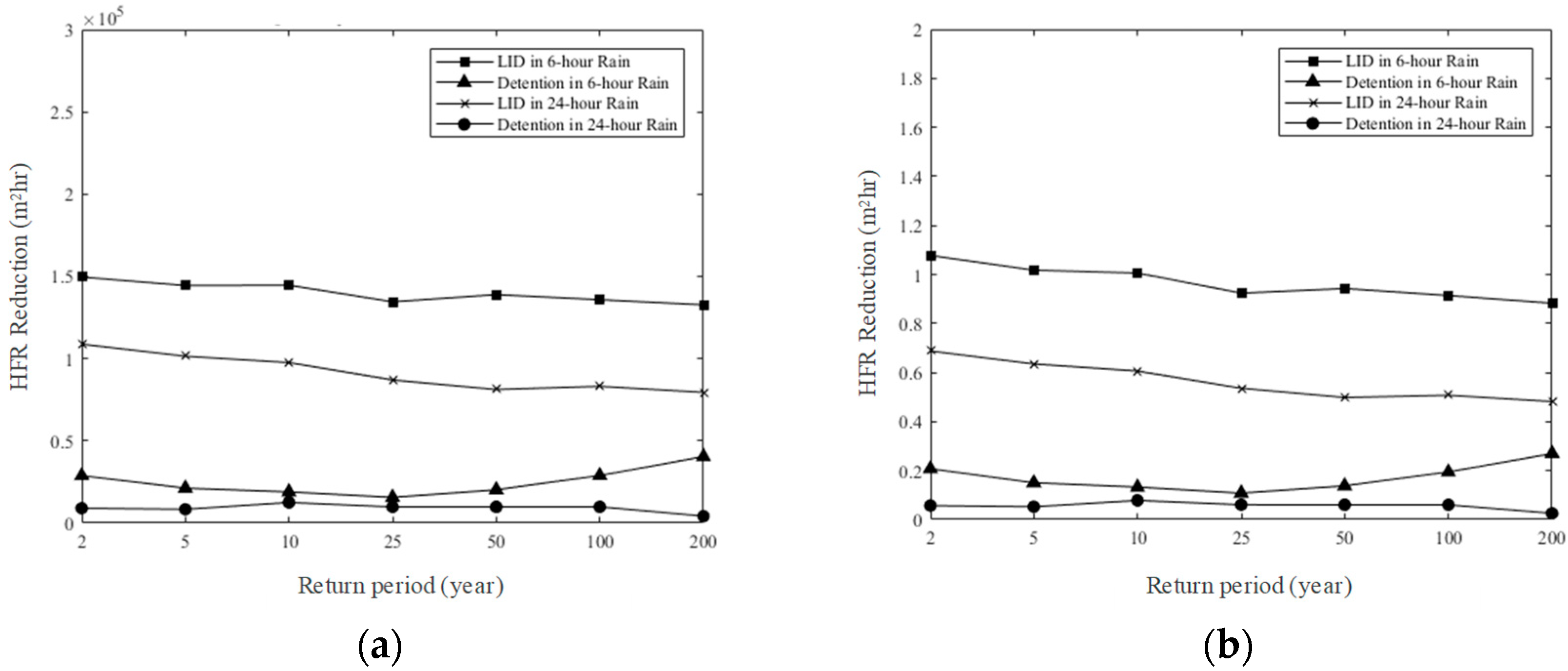
The HFR could be reduced by LIDs with increasing return periods for six-hour duration, but the amount of variation was not significant (
Figure 5). The HFR reduced by detention ponds roughly increased with the return periods. There was no significant change for different periods, but the overall performance was far less than LIDs. For six-hour duration, there was no particular relationship between the HFR reduction and the return periods. For 24-hour duration, LIDs reduced the HFR with 70% of the amount of the six-hour duration. The performance of detention ponds was low for the HFR reduction. Overall, the reduction rate and the reduction amount for different periods were mostly similar. The detention ponds could efficiently reduce the flood peak but not for the HFR. The main reason for which was the different mechanism of the storm control. The detention pond accumulated the surface runoff during the flood peak in a certain place and released it to the downstream after the flood peak, which would have an adverse effect on the downstream. In other words, the HFR could be reduced before the flood peak but be increased after it. The overall HFR reduction was small. LIDs increased infiltration and fundamentally reduced the surface runoff; therefore, the runoff could be reduced throughout the event and the overall HFR could also be reduced. LIDs comparing to detention ponds were proper practices to mitigate the impact toward the downstream.
The aforementioned results present that LIDs could control the storm event under the short duration better than the long duration in the urban area. Those simulations were done based on the adaptive distribution of LIDs and all components were conducted. For LID practices, it was necessary to evaluate the performance of each component, and select the best efficiency one as the priority. In order to explore the performance of the flood reduction for each component, every LID component was simulated individually, and was fully distributed to the available spaces within the region. The performance of each component was judged by the reduction rate per component area and per component cost.
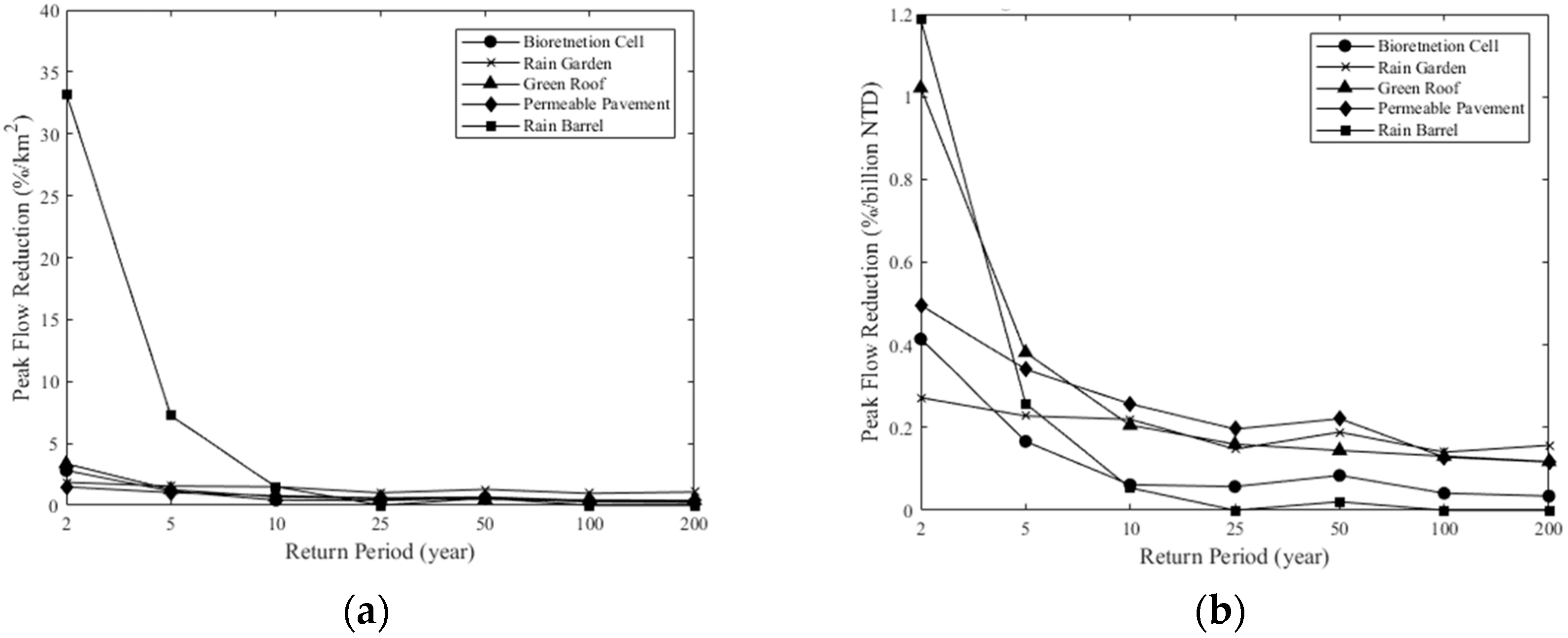
Figure 6 shows the results for the six-hour duration. The rain barrel had the highest reduction rate per area, but after a 10-year return period it did not show an obvious advantage (see
Figure 6a). The other LID components were far less effective than the rain barrel. In terms of the reduction rate per cost, the green roof and the permeable pavement performed better than others (see
Figure 6b). Before the 10-year return period, the green roof performed better than the permeable pavement, but after that the permeable pavement was better. It also showed that the permeable pavement was less affected by the return periods. Liang et al. [
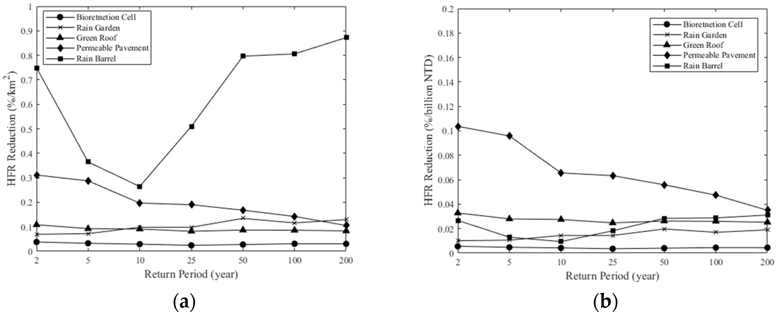
24] indicate that the selection of one LID component over the others highly depends on the return period and the duration. If the unit area and the unit cost were considered at the same time, the rain barrel could simultaneously reach the lesser area and cost but a larger flood reduction rate. The green roof had the low construction cost, but it needed a lot of space to reach the effective flood peak reduction. For the HFR reduction rate of each component per area, it showed that regardless of the return periods, the rain barrel still maximized the benefit compared to others and even performed better in high return periods (see
Figure 7a). The permeable pavement was second but the effect of reducing the HFR per area decreased with the increase of the return period. In terms of the HFR reduction rate per cost, the permeable pavement was the most advantageous regardless of the return period (See
Figure 7b). The rain barrel performed better in the low return period than the green roof, the rain garden, and the bioswale, but the green roof performed better in the high return period.
If the maximum efficiency to reduce the flood peak and the HFR in a limited area is the target, the rain barrel should be the best choice and then followed by the permeable pavement. If the cost is the main concern, the priority should be given to the permeable pavement and then followed by the green roof and the rain barrel. The rain barrel can obtain the large surface runoff per component area, but it is expensive. On the other hand, the permeable pavement and the green roof can obtain their own areas of the surface runoff, and replace the land which has a high impermeable rate, but the cost is inexpensive. In the simulation cases they performed second compared to the rain barrel. The bioswale could only be installed in places with low impermeable rates, and these places had less surface runoff. If the benefits of each LID component were compared under different conditions, it could be found that the proper LID component could perform much better than others under the low return period. This indicated the importance of the optimization for the LID distribution.
4.2. Optimization Method of LID Distribution
Installation of a large number of LIDs in the city is very costly. The prioritization of LIDs is important to ensure the maximum efficiency during storm events. The cost usually will be proportional to the reduction of the water volume. Therefore, this study showed how to achieve the maximum flood reduction through the LID optimization in highly developed regions without changing the original land use design. The MOGA was used to explore the prioritization of LIDs under different costs to reach the maximum reduction of the flood peak and the HFR. The existing administrative partitions of the study region were complicated and fragmented (there were 163 in total), therefore we considered the geographical location, the population size, and the simulation time, and then reorganized them into 53 partitions. We ensured that each partition contained 10,000 people, and the optimization would calculate the ratio of area including LIDs for each partition. The ratio was defined as the area including LIDs dividing the available space. In order to enhance the simulation efficiency and avoid the fragmented configuration, we started with the ratio, allocated LIDs in this partition, and then performed the optimization. The updated ratio was then applied in the new iteration. The calculation was continued until the optimal ratio was reached.
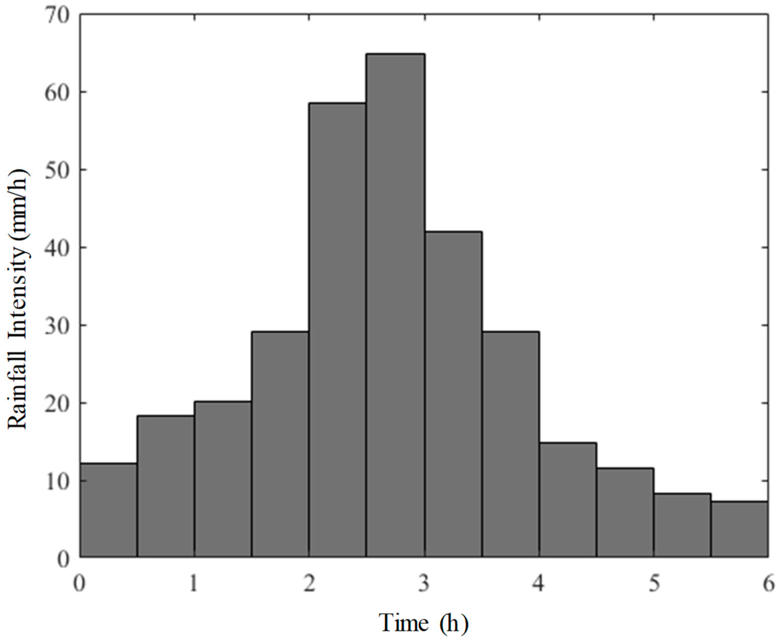
The effect of different intensity rainfall on LID was analyzed and showed that using LIDs could successfully reduce the flood peak for the low return period. The scenario was then designed with six-hour duration and five-year return period to assess the LID optimal ratio of each partition (
Figure 8). The five-year return period is usually the designed criteria for urban drainage systems. Detention ponds were usually limited by the space and the selection was also limited, and LIDs were flexible and could apply appropriate components according to the different land uses, therefore, only the spatial configuration of the LID components was discussed, regardless of the configuration of the detention ponds. In this study, MOGA function “gamultiobj” in MATLAB r2017a was conducted to do optimization. The setting variable was the ratio of area including LIDs for each partition, and the objective function was the reduction of the flood peak and the LID cost, or the reduction of the HFR and the LID cost. The flood peak flow data was obtained directly by SWMM simulation, while the HFR was calculated indirectly by SWMM simulation of the water depth sequence of the major drainages. The cost of LID configuration was estimated based on the LID manual. The remaining parameters, such as the number of contemporary individuals was 200, the best individual rate was 0.15, the use of the single-point mating method, the mating rate was 0.8, and the mutation rate was 0.05. Finally, when the average propagation value was less than 0.0001 or the total generation was greater than 2000, the calculation was stopped and five times the evaluation was calculated to check the result sufficiently converged.
4.3. The Spatial Configuration of the LID from Optimization
The previous sections showed that the performance of LIDs would be affected by the rainfall intensity and the duration. The configuration of LID in different locations was investigated to learn the impacts on the reduction. If we allowed the maximum area to place a specific LID component, calculated the reduction of the flood peak or the HFR, and then divided the cost for each partition in the study region, we could simply decide the priority based on this result without the optimization. However, the different combinations of the ratio of LIDs in each partition would have interacted effects for the reduction. In addition, there was no means to decide how many LIDs should be set in partitions of the region under the specific budget. Therefore, in this study the different ratios of the LID configuration and the different LID components in each partition were calculated with the MOGA method to obtain the optimized LID distribution for the region under the specific budget.
Without setting LID in the study region the flood peak flow was 176 m
3/s and this was defined as 100% of the peak flow. If we assumed each partition could contain the maximum area of the LID, the total cost would be
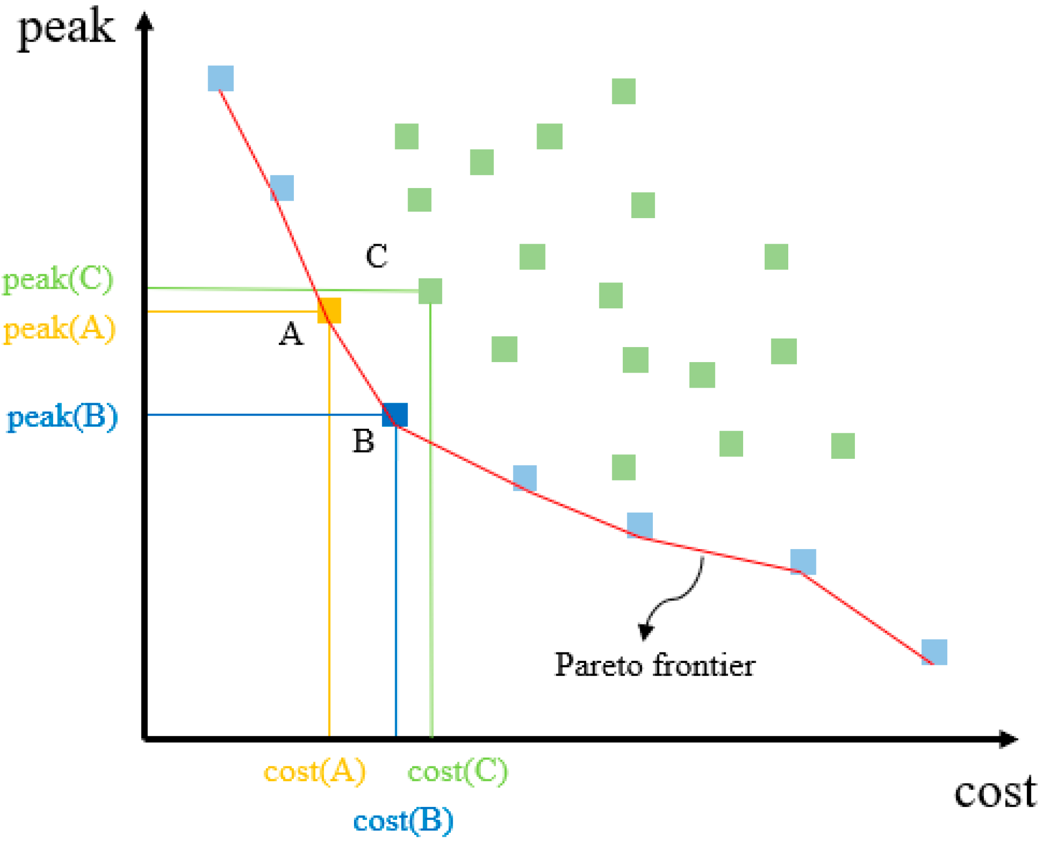
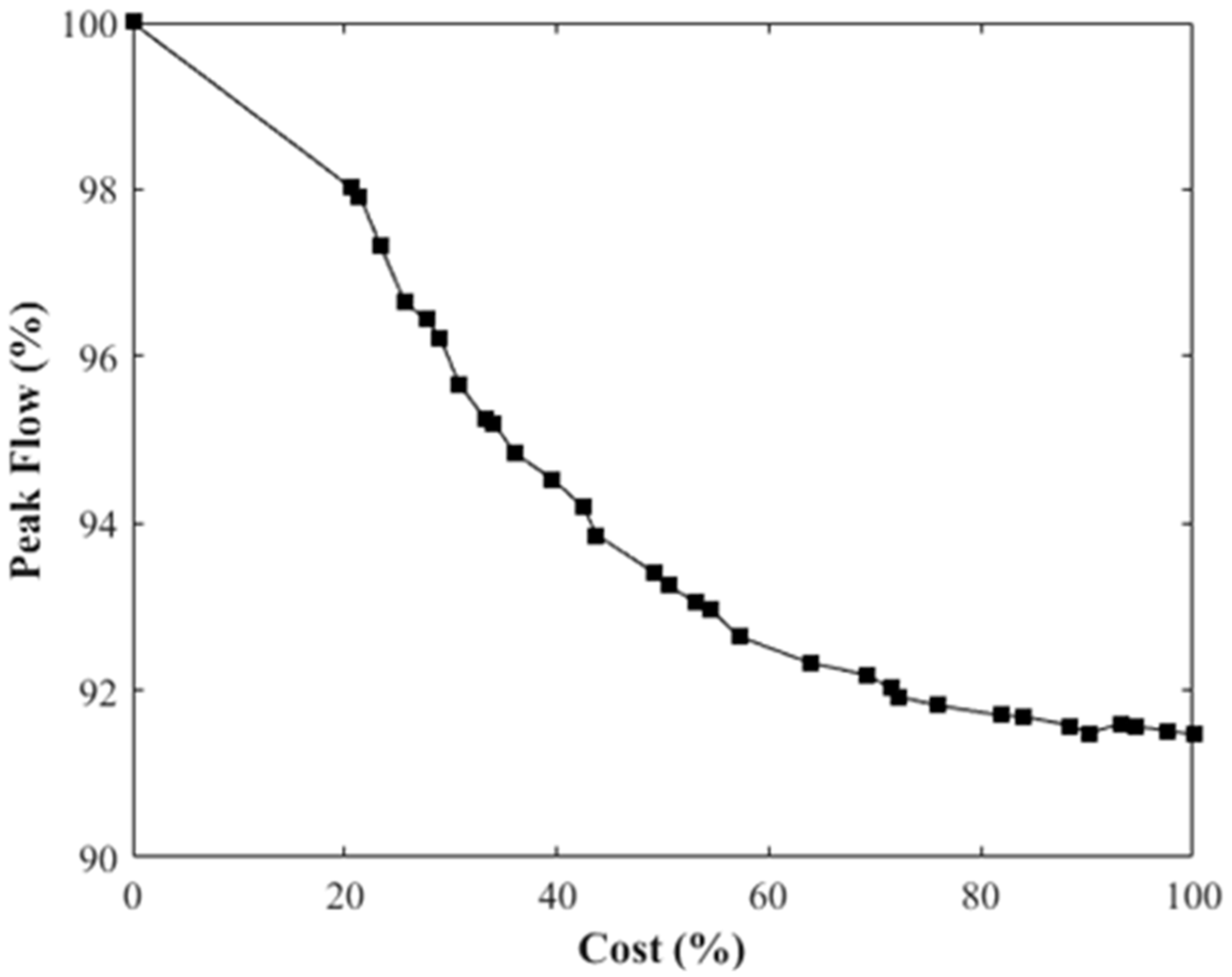
$1.1 billion which defined as 100% of the LID cost (the cost was estimated based on the LID manual). After the MOGA simulation, the Pareto frontier between the peak flow and the cost was obtained (see
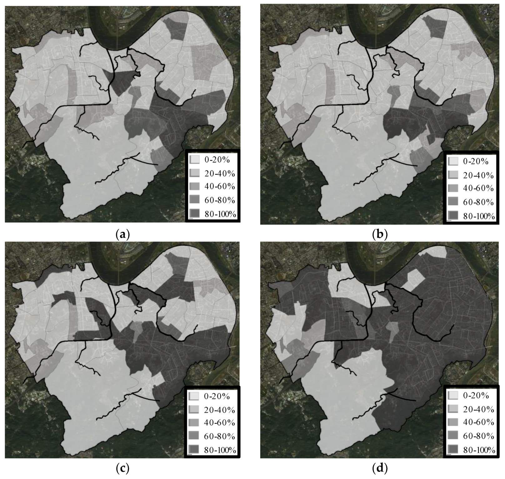
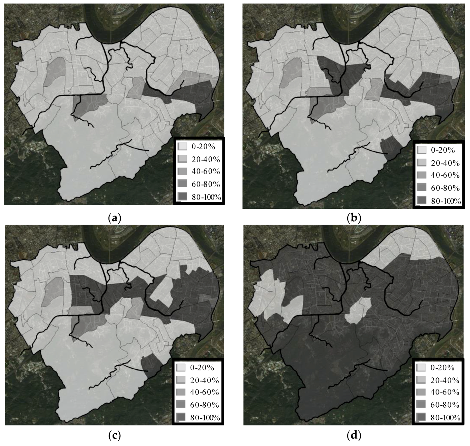
Figure 9). It showed that when the cost of the LID was more than 80%, the flood peak flow was almost the same as the 100% cost. This meant that with the LIDs setting up to 80% the flood reduction might reach the maximum for this region. In terms of optimal spatial configuration, the priority of the partitions to set the LIDs under different costs is shown in
Figure 10. The darker partition means the higher benefit and the higher priority to set the LID. From
Figure 10a, it showed that the east side should be placed with LID before the west side. For 50% cost, the higher priority partitions to set the LID were near the middle and the upstream of the drainage and sewerage system (
Figure 10c). When setting a cost of up to 80%, the lower priority LID configuration areas were the upstream mountainous area and the downstream of the major drainage and the sewerage system (
Figure 10d).
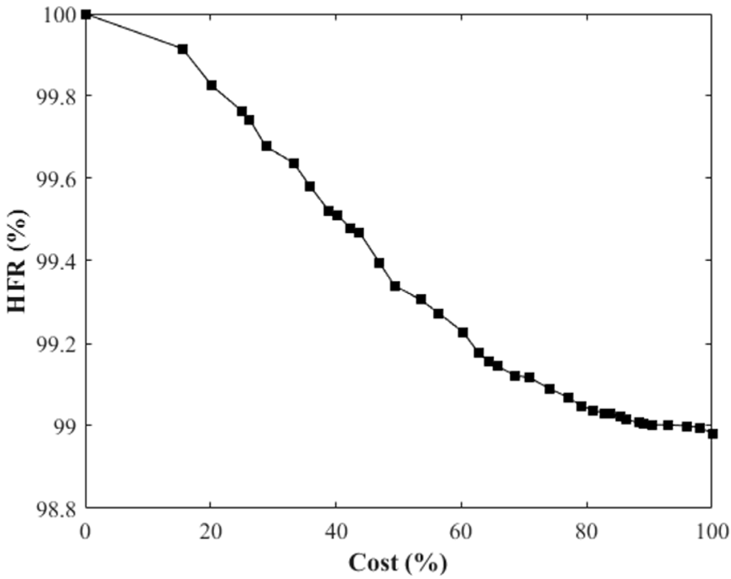
The Pareto frontier between the cost and the HFR is shown in
Figure 11. It also showed that when the cost of the LID was more than 80%, the HRF was almost the same as the 100%. In terms of optimal spatial configuration for the HFR, the priority of the partitions to set the LIDs under different costs is shown in
Figure 12. From the 30%–50% cost, the result indicated that the upstream of the major drainage and sewerage system had the higher priority. Therefore, if the cost, the flood peak reduction and the HFR reduction were taken into account at the same time, the highest priority should have been the area in the middle of the major drainage, followed by the upstream of the major drainage, and avoided the area which was allocated to the downstream of the drainage.
4.4. Monte Carlo Method
For discussing the optimization of the LID distribution, it may be limited to find the proper area near the upstream or downstream in the major drainage. However, the sewerage system in the city was intricate and it was difficult to define the upstream and downstream areas. It was necessary to configure the LID with other considerations. The aforementioned results showed that although the major drainage two and three can deliver the same discharge, the LID configurations were prone to be placed near the middle and upstream of the drainage two instead of the drainage three. It entailed that there were other factors affecting the optimal setting of LIDs. The Monte Carlo test was conducted to estimate the effect of the land use for the LID configuration in this section. We randomly assigned the land use toward different sub-catchments and the probability of various land use was the same as the original plan (
Table 4). The average impermeable rate of each partition was applied to represent the degree of the development. The higher impermeable rate meant the higher degree of the development. In this test the optimal allocation ratio was also estimated to find out the correlation to the degree of the development.
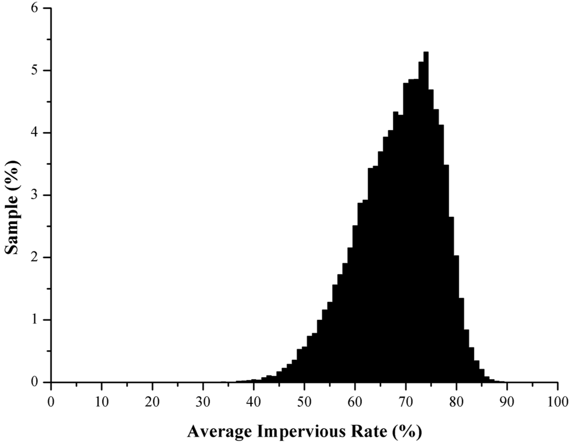
Land use and zoning can be reclassified, therefore the 53 partitions were merged into 23 partitions to reduce the computational time. This experiment produced a total of 2259 sets of samples, so there was a total of 51,957 impermeable rate samples. The distribution percentage of these 51,957 samples is shown in
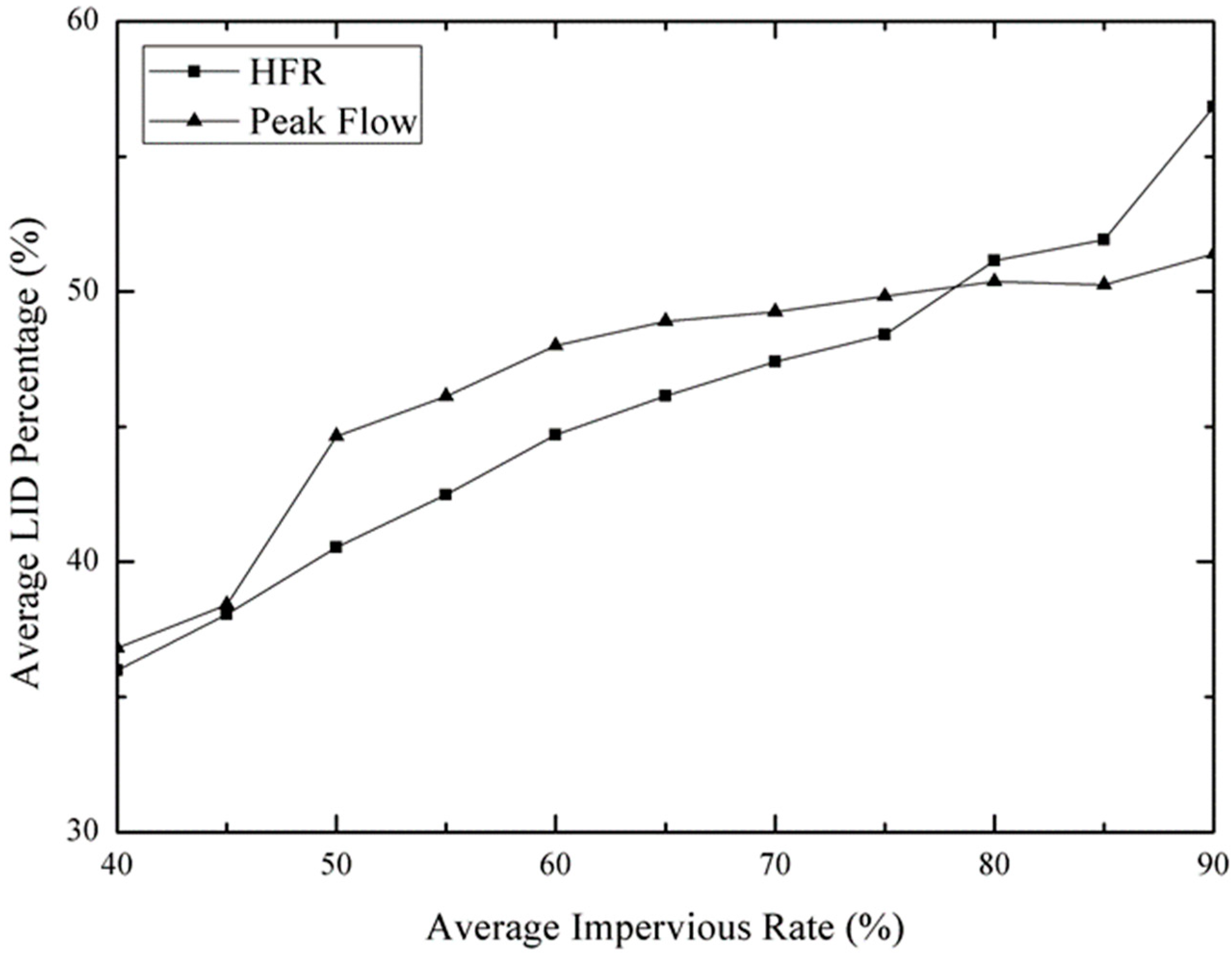
Figure 13. A positive correlation was uncovered between the optimal allocation ratio and the impermeable rate of the partition, no matter if the goal was to reduce the flood peak or the HRF (see
Figure 14). If the average impervious rate was below 50%, the performance of LIDs to reduce the flood peak significantly decreased. It meant that the LID setting should be placed in the area where impervious rate was high to obtain the best performance. For the HFR, the result also showed that the highly developed regions needed to set up LIDs to reduce the HFR. The LID distribution result with the Monte Carlo test showed that the LID location in the drainage system was less related to the flood reduction but would affect the HFR reduction. In other words, in terms of the flood reduction, the degree of development could be utilized as the efficient judgment to the LID distribution. Moreover, for urban designers this experiment can be a guideline for the comprehensive planning or the rezoning of the land to include the LID design.
