Steric Sea Level Changes from Ocean Reanalyses at Global and Regional Scales


Abstract
1. Introduction
1.1. Sea Level Rise as a Proxy of Climate Change and Threat from Global Warming
1.2. Methods of Estimation of Sea Level
1.3. Overview of Reanalyses Performances in Capturing Sea Level Variability
1.4. Using Reanalyses to Partition Causes of Sea Level Variability
2. Material and Methods
2.1. Formulation of the Sea Level Balance
2.2. Datasets Used in the Present Work
3. Steric Sea Level Trends in Centennial Reanalyses
3.1. Preliminary Validation
3.2. Centennial Trends
4. Contemporary Sea Level Change from Ocean Reanalyses
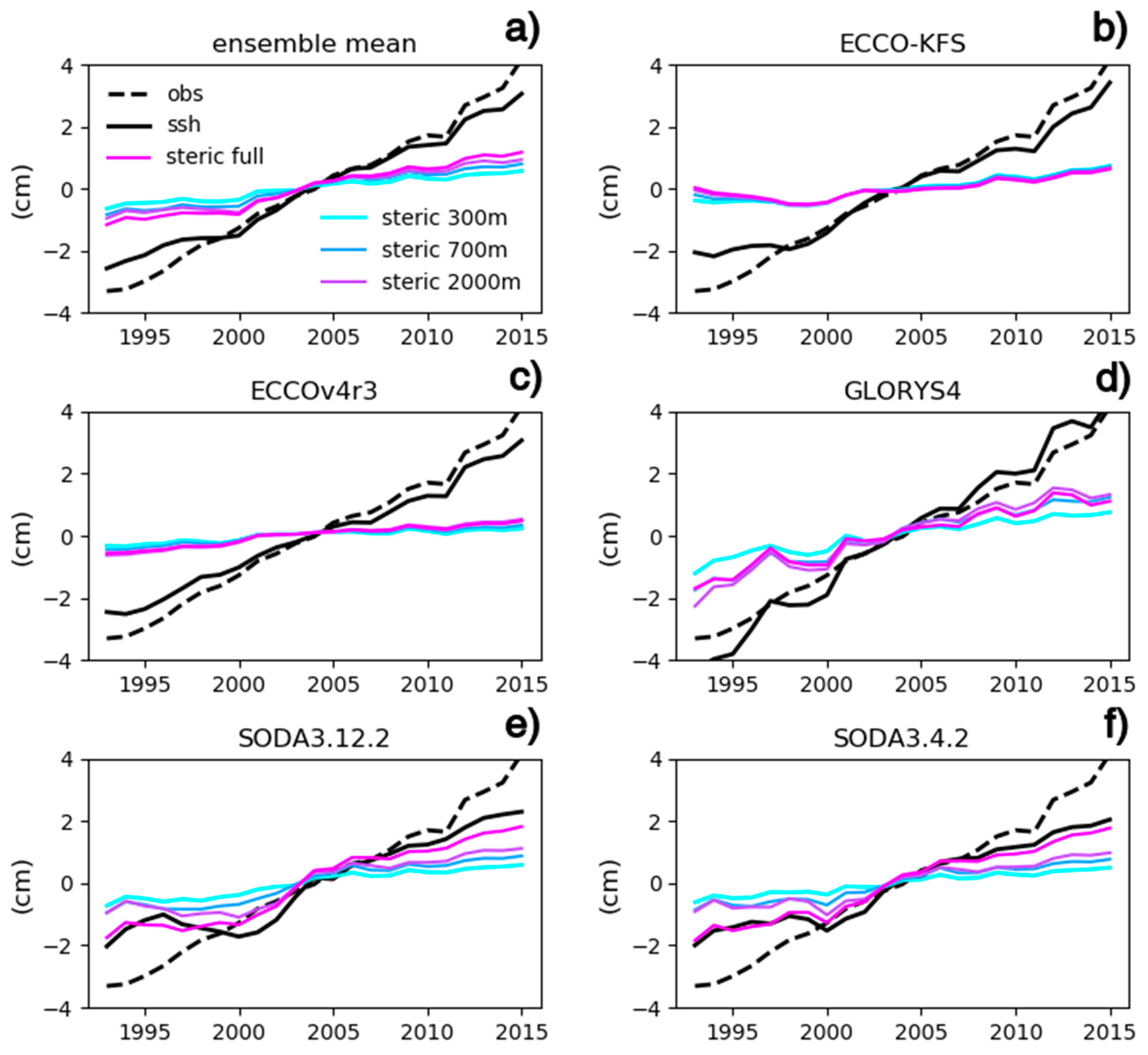
4.1. Assessment of Reanalyses
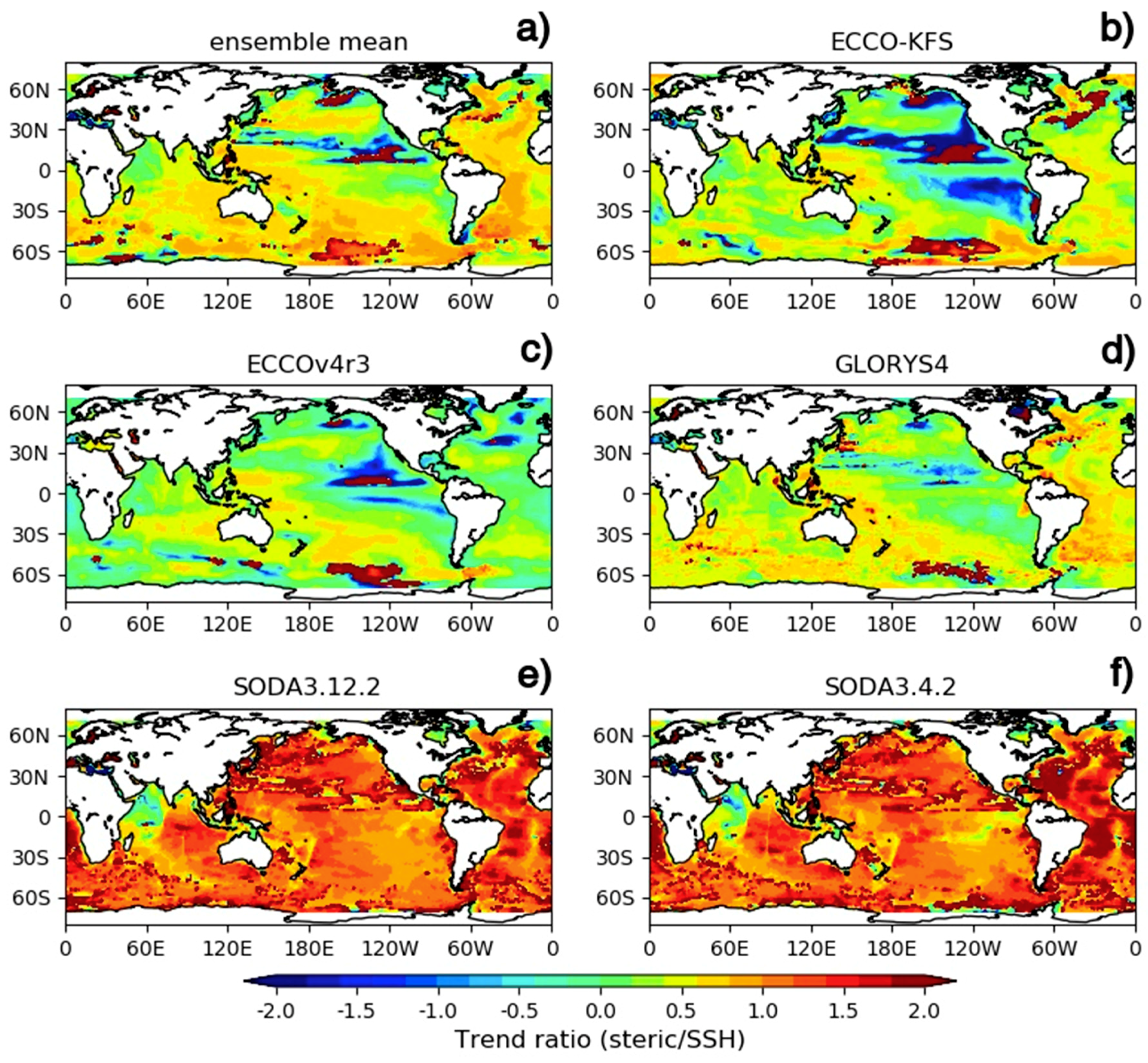
4.2. Contribution of Steric Sea Level to Sea Surface Height Trends
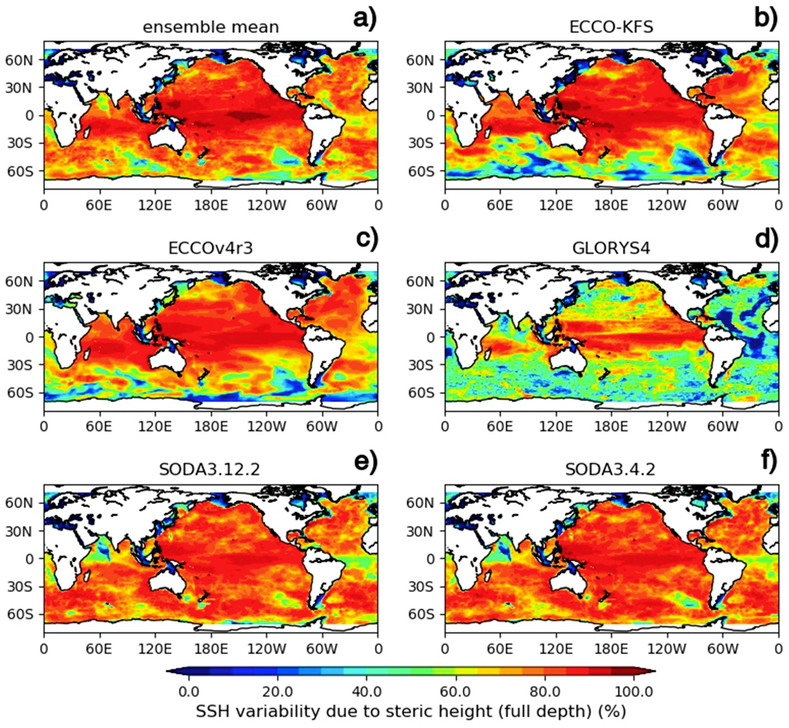
4.3. Inter-Annual Variability
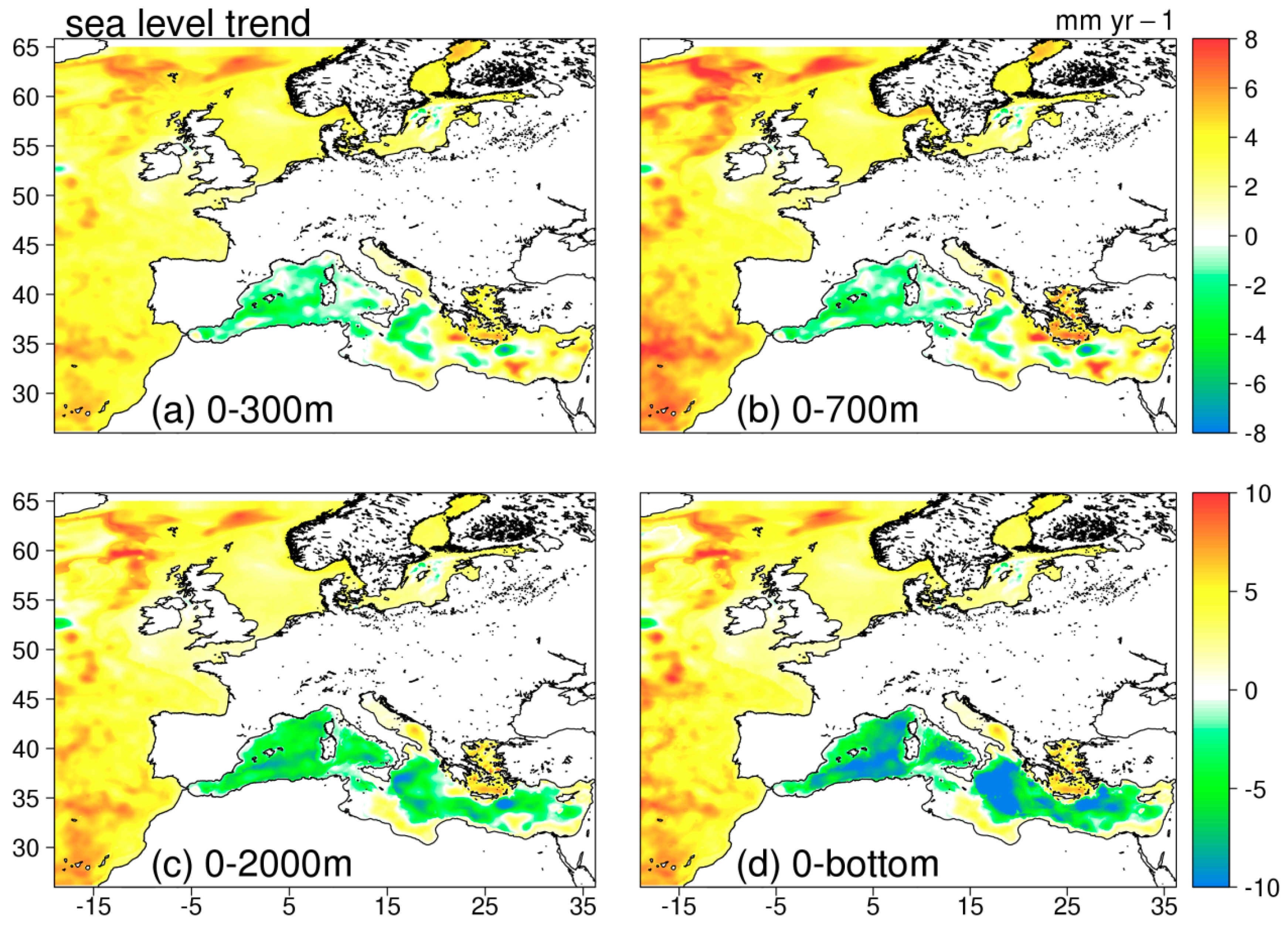
4.4. Sea-Level Trends in Regional Reanalyses for the European Seas
5. Summary and Discussion
Supplementary Materials
Author Contributions
Funding
Acknowledgments
Conflicts of Interest
References
- von Schuckmann, K.; Le Traon, P.Y.; Alvarez-Fanjul, E.; Axell, L.; Balmaseda, M.; Breivik, L.A.; Brewin, R.J.; Bricaud, C.; Drevillon, M.; Drillet, Y.; et al. The Copernicus Marine Environment Monitoring Service Ocean State Report. J. Oper. Oceanogr. 2016, 9, S235–S320. [Google Scholar] [CrossRef]
- von Schuckmann, K.; Le Traon, P.Y.; Smith, N.; Pascual, A.; Brasseur, P.; Fennel, K.; Djavidnia, S.; Aaboe, S.; Fanjul, E.A.; Autret, E.; et al. Copernicus Marine Service Ocean State Report. J. Oper. Oceanogr. 2018, 11, S1–S142. [Google Scholar] [CrossRef]
- Lichter, M.; Vafeidis, A.T.; Nicholls, R.J.; Kaiser, G. Exploring data-related uncertainties in analyses of land area and population in the ‘low-elevation coastal zone’ (LECZ). J. Coast. Res. 2011, 27, 757–768. [Google Scholar] [CrossRef]
- Menéndez, M.; Woodworth, P.L. Changes in extreme high water levels based on a quasi-global tide-gauge data set. J. Geophys. Res. Space Phys. 2010, 115. [Google Scholar] [CrossRef]
- Feng, X.; Tsimplis, M.N. Sea level extremes at the coasts of China. J. Geophys. Res. Ocean. 2014, 119, 1593–1608. [Google Scholar] [CrossRef]
- Stammer, D.; Cazenave, A.; Ponte, R.M.; Tamisiea, M.E. Causes for Contemporary Regional Sea Level Changes. Annu. Rev. Mar. Sci. 2013, 5, 21–46. [Google Scholar] [CrossRef] [PubMed]
- Munk, W. Twentieth century sea level: An enigma. Proc. Natl. Acad. Sci. USA 2002, 99, 6550–6555. [Google Scholar] [CrossRef]
- Piecuch, C.G.; Heimbach, P.; Ponte, R.M.; Forget, G. Sensitivity of contemporary sea level trends in a global ocean state estimate to effects of geothermal fluxes. Ocean Model. 2015, 96, 214–220. [Google Scholar] [CrossRef]
- Ablain, M.; Meyssignac, B.; Zawadzki, L.; Jugier, R.; Ribes, A.; Cazenave, A.; Picot, N. Uncertainty in Satellite estimate of Global Mean Sea Level changes, trend and acceleration. Earth Syst. Sci. Data Discuss. 2019. [Google Scholar] [CrossRef]
- Cazenave, A.; Meyssignac, B.; Palanisamy, H. Global Sea Level Budget Assessment by World Climate Research Programme. Seanoe 2018. [Google Scholar] [CrossRef]
- WCRP Global Sea Level Budget Group. Global sea-level budget 1993-present. Earth Syst. Sci. Data 2018, 10, 1551–1590. [Google Scholar] [CrossRef]
- Chen, X.; Zhang, X.; Church, J.A.; Watson, C.S.; King, M.A.; Monselesan, D.; Legresy, B.; Harig, C. The increasing rate of global mean sea-level rise during 1993–2014. Nat. Clim. Chang. 2017, 7, 492–495. [Google Scholar] [CrossRef]
- Suzuki, T.; Ishii, M. Regional distribution of sea level changes resulting from enhanced greenhouse warming in the Model for Interdisciplinary Research on Climate version 3.2. Geophys. Res. Lett. 2011, 38, 601. [Google Scholar] [CrossRef]
- Church, J.A.; Gregory, J.M.; White, N.J.; Platten, S.M.; Mitrovica, J.X. Understanding and projecting sea level change. Oceanography 2011, 24, 130–143. [Google Scholar] [CrossRef]
- Dong, L.; Zhou, T. Steric sea level change in twentieth century historical climate simulation and IPCC-RCP8.5 scenario projection: A comparison of two versions of FGOALS model. Adv. Atmos. Sci. 2013, 30, 841–854. [Google Scholar] [CrossRef]
- IPCC. Contribution of working group I to the fifth assessment report of the intergovernmental panel on climate change. In Climate Change 2013: The Physical Science Basis; Cambridge University Press: Cambridge, UK; New York, NY, USA, 2013; p. 1535. [Google Scholar]
- Clark, P.U.; Church, J.A.; Gregory, J.M.; Payne, A.J. Recent Progress in Understanding and Projecting Regional and Global Mean Sea Level Change. Curr. Clim. Chang. Rep. 2015, 1, 224–246. [Google Scholar] [CrossRef]
- Hu, A.; Bates, S.C. Internal climate variability and projected future regional steric and dynamic sea level rise. Nat. Commun. 2018, 9, 1068. [Google Scholar] [CrossRef] [PubMed]
- Terada, M.; Minobe, S. Projected sea level rise, gyre circulation and water mass formation in the western North Pacific: CMIP5 inter-model analysis. Clim. Dyn. 2018, 50, 4767. [Google Scholar] [CrossRef]
- Pardaens, A.K.; Gregory, J.M.; Lowe, J. A model study of factors influencing projected changes in regional sea level over the twenty-first century. Clim. Dyn. 2011, 36, 2015–2033. [Google Scholar] [CrossRef]
- Vousdoukas, M.I.; Mentaschi, L.; Voukouvalas, E.; Verlaan, M.; Jevrejeva, S.; Jackson, L.P.; Feyen, L. Global probabilistic projections of extreme sea levels show intensification of coastal flood hazard. Nat. Commun. 2018, 9, 2360. [Google Scholar] [CrossRef]
- Nowicki, S.; Seroussi, H. Projections of Future Sea Level Contributions from the Greenland and Antarctic Ice Sheets: Challenges Beyond Dynamical Ice Sheet Modeling. Oceanography 2018, 31, 109–117. [Google Scholar] [CrossRef]
- MacIntosh, C.R.; Merchant, C.J.; von Schuckmann, K. Uncertainties in Steric Sea Level Change Estimation During the Satellite Altimeter Era: Concepts and Practices. In Integrative Study of the Mean Sea Level and Its Components; Cazenave, A., Champollion, N., Paul, F., Benveniste, J., Eds.; Springer: Berlin, Germany, 2017; Volume 58. [Google Scholar]
- Church, J.A.; Roemmich, D.; Domingues, C.M.; Willis, J.K.; White, N.J.; Gilson, J.E.; Stammer, D.; Köhl, A.; Chambers, D.P.; Landerer, F.W.; et al. Ocean Temperature and Salinity Contributions to Global and Regional Sea-Level Change. In Understanding Sea-Level Rise and Variability; Church, J.A., Woodworth, P.L., Aarup, T., Wilson, W.S., Eds.; Cambridge University Press: Cambridge, UK, 2010; pp. 143–176. [Google Scholar]
- Levitus, S.; Antonov, J.I.; Boyer, T.P.; Garcia, H.E.; Locarnini, R.A. Linear trends of zonally averaged thermosteric, halosteric, and total steric sea level for individual ocean basins and the world ocean, (1955–1959)–(1994–1998). Geophys. Res. Lett. 2005, 32, L16601. [Google Scholar] [CrossRef]
- Ishii, M.; Kimoto, M.; Sakamoto, K.; Iwasaki, S.I. Steric sea level changes estimated from historical ocean subsurface temperature and salinity analyses. J. Oceanogr. 2006, 62, 155–170. [Google Scholar] [CrossRef]
- Gille, S.T. Decadal-Scale Temperature Trends in the Southern Hemisphere Ocean. J. Clim. 2008, 21, 4749–4765. [Google Scholar] [CrossRef]
- Sallée, J.-B.; Cnrs, L.-I. Southern Ocean Warming. Oceanography 2018, 31, 52–62. [Google Scholar] [CrossRef]
- Chang, Y.-S.; Vecchi, G.A.; Rosati, A.; Zhang, S.; Yang, X. Comparison of global objective analyzed T-S fields of the upper ocean for 2008–2011. J. Mar. Syst. 2014, 137, 13–20. [Google Scholar] [CrossRef]
- Levitus, S.; Antonov, J.I.; Boyer, T.P.; Locarnini, R.A.; Garcia, H.E.; Mishonov, A.V. Global ocean heat content 1955–2007 in light of recently revealed instrumentation problems. Geophys. Res. Lett. 2009, 36, L07608. [Google Scholar]
- Cheng, L.; Luo, H.; Boyer, T.; Cowley, R.; Abraham, J.; Gouretski, V.; Reseghetti, F.; Zhu, J. How Well Can We Correct Systematic Errors in Historical XBT Data? J. Atmos. Ocean. Technol. 2018, 35, 1103–1125. [Google Scholar] [CrossRef]
- Church, J.A.; White, N.J.; Coleman, R.; Lambeck, K.; Mitrovica, J.X. Estimates of the Regional Distribution of Sea Level Rise over the 1950–2000 Period. J. Clim. 2004, 17, 2609–2625. [Google Scholar] [CrossRef]
- Carson, M.; Köhl, A.; Stammer, D.; Meyssignac, B.; Church, J.; Schröter, J.; Wenzel, M.; Hamlington, B. Regional Sea Level Variability and Trends, 1960–2007: A Comparison of Sea Level Reconstructions and Ocean Syntheses. J. Geophys. Res. Oceans 2017, 122, 9068–9091. [Google Scholar] [CrossRef]
- Legeais, J.-F.; Ablain, M.; Zawadzki, L.; Zuo, H.; Johannessen, J.A.; Scharffenberg, M.G.; Fenoglio-Marc, L.; Fernandes, M.J.; Andersen, O.B.; Rudenko, S.; et al. An improved and homogeneous altimeter sea level record from the ESA Climate Change Initiative. Earth Syst. Sci. Data 2018, 10, 281–301. [Google Scholar] [CrossRef]
- Chelton, D.B.; Ries, J.C.; Haines, B.J.; Fu, L.L.; Callahan, P.S. Satellite altimetry. In Satellite Altimetry and Earth Sciences: A Handbook of Techniques and Applications; Fu, L.L., Cazenave, A., Eds.; Academic Press: San Diego, CA, USA, 2001; pp. 1–132. [Google Scholar]
- Forget, G.; Ponte, R.M. The partition of regional sea level variability. Prog. Oceanogr. 2015, 137, 173–195. [Google Scholar] [CrossRef]
- Leuliette, E.W.; Miller, L. Closing the sea level rise budget with altimetry, Argo, and GRACE. Geophys. Res. Lett. 2009, 36, 608. [Google Scholar] [CrossRef]
- Garcia-Garcia, D.; Chao, B.F.; Boy, J.-P.; García-García, D. Steric and mass-induced sea level variations in the Mediterranean Sea revisited. J. Geophys. Res. Space Phys. 2010, 115, 016. [Google Scholar] [CrossRef]
- Kleinherenbrink, M.; Riva, R.; Sun, Y. Sub-basin-scale sea level budgets from satellite altimetry, Argo floats and satellite gravimetry: A case study in the North Atlantic Ocean. Ocean Sci. 2016, 12, 1179–1203. [Google Scholar] [CrossRef]
- Storto, A.; Masina, S.; Balmaseda, M.; Guinehut, S.; Xue, Y.; Szekely, T.; Fukumori, I.; Forget, G.; Chang, Y.-S.; Good, S.A.; et al. Steric sea level variability (1993–2010) in an ensemble of ocean reanalyses and objective analyses. Clim. Dyn. 2017, 1–21. [Google Scholar] [CrossRef]
- Storto, A.; Masina, S.; Simoncelli, S.; Iovino, D.; Cipollone, A.; Drevillon, M.; Drillet, Y.; von Schuckman, K.; Parent, L.; Garric, G.; et al. The added value of the multi-system spread information for ocean heat content and steric sea level investigations in the CMEMS GREP ensemble reanalysis product. Clim. Dyn. 2019, 53, 287. [Google Scholar] [CrossRef]
- Lombard, A.; Garric, G.; Penduff, T. Regional patterns of observed sea level change: Insights from a 1/4 global ocean/sea-ice hindcast. Ocean Dyn. 2009, 59, 433–449. [Google Scholar] [CrossRef]
- Kuhlbrodt, T.; Gregory, J.M. Ocean heat uptake and its consequences for the magnitude of sea level rise and climate change. Geophys. Res. Lett. 2012, 39, L18608. [Google Scholar] [CrossRef]
- Balmaseda, M.A.; Mogensen, K.; Weaver, A.T. Evaluation of the ECMWF ocean reanalysis system ORAS4. Q. J. R. Meteorol. Soc. 2013, 139, 1132–1161. [Google Scholar] [CrossRef]
- Kohl, A.; Stammer, D.; Cornuelle, B. Interannual to Decadal Changes in the ECCO Global Synthesis. J. Phys. Oceanogr. 2007, 37, 313–337. [Google Scholar] [CrossRef]
- Church, J.A.; Clark, P.U.; Cazenave, A.; Gregory, J.M.; Jevrejeva, S.; Levermann, A.; Merrifield, M.A.; Milne, G.A.; Nerem, R.S.; Nunn, P.D.; et al. Sea Level Change. In Climate Change 2013: The Physical Science Basis. Contribution of Working Group I to the Fifth Assessment Report of the Intergovernmental Panel on Climate Change; Stocker, T.F., Qin, D., Plattner, G.-K., Tignor, M., Allen, S.K., Boschung, J., Nauels, A., Xia, Y., Bex, V., Midgley, P.M., Eds.; Cambridge University Press: Cambridge, UK; New York, NY, USA, 2013. [Google Scholar]
- Yin, J.; Griffies, S.M.; Stouffer, R.J. Spatial Variability of Sea Level Rise in Twenty-First Century Projections. J. Clim. 2010, 23, 4585–4607. [Google Scholar] [CrossRef]
- Storto, A.; Alvera-Azcárate, A.; Balmaseda, M.A.; Barth, A.; Chevallier, M.; Counillon, F.; Domingues, C.M.; Drevillon, M.; Drillet, Y.; Forget, G.; et al. Ocean reanalyses: Recent advances and unsolved challenges. Front. Mar. Sci. 2019. [Google Scholar] [CrossRef]
- Stammer, D.; Balmaseda, M.; Heimbach, P.; Kohl, A.; Weaver, A. Ocean Data Assimilation in Support of Climate Applications: Status and Perspectives. Annu. Rev. Mar. Sci. 2016, 8, 491–518. [Google Scholar] [CrossRef]
- Heimbach, P.; Fukumori, I.; Hill, C.N.; Ponte, R.M.; Stammer, D.; Wunsch, C.; Campin, J.-M.; Cornuelle, B.; Fenty, I.; Forget, G.; et al. Putting It All Together: Adding Value to the Global Ocean and Climate Observing Systems With Complete Self-Consistent Ocean State and Parameter Estimates. Front. Mar. Sci. 2019, 6, 55. [Google Scholar] [CrossRef]
- Yang, C.; Masina, S.; Bellucci, A.; Storto, A. The rapid warming of the North Atlantic Ocean in the mid-1990s in an eddy permitting ocean reanalysis (1982–2013). J. Clim. 2016, 29, 5417–5430. [Google Scholar] [CrossRef]
- Carton, J.A.; Penny, S.G.; Kalnay, E. Temperature and Salinity Variability in the SODA3, ECCO4r3, and ORAS5 Ocean Reanalyses, 1993–2015. J. Clim. 2019, 32, 2277–2293. [Google Scholar] [CrossRef]
- Uotila, P.; Goosse, H.; Haines, K.; Chevallier, M.; Barthélemy, A.; Bricaud, C.; Carton, J.; Fučkar, N.; Garric, G.; Iovino, D.; et al. An assessment of ten ocean reanalyses in the polar regions. Clim. Dyn. 2019, 52, 1613–1650. [Google Scholar] [CrossRef]
- Carton, J.A.; Giese, B.S.; Grodsky, S.A. Sea level rise and the warming of the oceans in the Simple Ocean Data Assimilation (SODA) ocean reanalysis. J. Geophys. Res. Space Phys. 2005, 110, C09006. [Google Scholar] [CrossRef]
- Yang, C.; Masina, S.; Storto, A. Historical ocean reanalyses (1900–2010) using different data assimilation strategies. Q. J. R. Meteorol. Soc. 2017, 143, 479–493. [Google Scholar] [CrossRef]
- Yang, C.; Storto, A.; Masina, S. Quantifying the effects of observational constraints and uncertainty in atmospheric forcing on historical ocean reanalyses. Clim. Dyn. 2019, 52, 3321. [Google Scholar] [CrossRef]
- Balmaseda, M.; Hernandez, F.; Storto, A.; Palmer, M.; Alves, O.; Shi, L.; Smith, G.; Toyoda, T.; Valdivieso, M.; Barnier, B.; et al. The Ocean Reanalyses Intercomparison Project (ORA-IP). J. Oper. Oceanogr. 2015, 8, S80–S97. [Google Scholar] [CrossRef]
- Chepurin, G.A.; Carton, J.A.; Leuliette, E. Sea level in ocean reanalyses and tide gauges. J. Geophys. Res. Oceans 2014, 119, 147–155. [Google Scholar] [CrossRef]
- Pfeffer, J.; Tregoning, P.; Purcell, A.; Sambridge, M. Multitechnique Assessment of the Interannual to Multidecadal Variability in Steric Sea Levels: A Comparative Analysis of Climate Mode Fingerprints. J. Clim. 2018, 31, 7583–7597. [Google Scholar] [CrossRef]
- Calafat, F.M.; Chambers, D.P.; Tsimplis, M.N. Mechanisms of decadal sea level variability in the eastern North Atlantic and the Mediterranean Sea. J. Geophys. Res. Space Phys. 2012, 117, C09022. [Google Scholar] [CrossRef]
- Forget, G.; Campin, J.-M.; Heimbach, P.; Hill, C.N.; Ponte, R.M.; Wunsch, C. ECCO version 4: An integrated framework for non-linear inverse modeling and global ocean state estimation. Geosci. Model Dev. 2015, 8, 3071–3104. [Google Scholar] [CrossRef]
- Piecuch, C.G.; Ponte, R.M. Mechanisms of Global-Mean Steric Sea Level Change. J. Clim. 2014, 27, 824–834. [Google Scholar] [CrossRef]
- Piecuch, C.G.; Ponte, R.M. Mechanisms of interannual steric sea level variability. Geophys. Res. Lett. 2011, 38, L15605. [Google Scholar] [CrossRef]
- Lu, Q.; Zuo, J.; Li, Y.; Chen, M. Interannual sea level variability in the tropical Pacific Ocean from 1993 to 2006. Glob. Planet. Chang. 2013, 107, 70–81. [Google Scholar] [CrossRef]
- Fukumori, I.; Wang, O. Origins of heat and freshwater anomalies underlying regional decadal sea level trends. Geophys. Res. Lett. 2013, 40, 563–567. [Google Scholar] [CrossRef]
- Köhl, A. Detecting Processes Contributing to Interannual Halosteric and Thermosteric Sea Level Variability. J. Clim. 2014, 27, 2417–2426. [Google Scholar] [CrossRef]
- Wunsch, C.; Ponte, R.M.; Heimbach, P. Decadal Trends in Sea Level Patterns: 1993–2004. J. Clim. 2007, 20, 5889–5911. [Google Scholar] [CrossRef]
- Wang, C.Z.; Dong, S.F.; Munoz, E. Seawater density variations in the North Atlantic and the Atlantic meridional overturning circulation. Clim. Dyn. 2010, 34, 953–968. [Google Scholar] [CrossRef]
- Gill, A.; Niller, P. The theory of the seasonal variability in the ocean. Deep Sea Res. Oceanogr. Abstr. 1973, 20, 141–177. [Google Scholar] [CrossRef]
- Griffies, S.M.; Greatbatch, R.J. Physical processes that impact the evolution of global mean sea level in ocean climate models. Ocean Model. 2012, 51, 37–72. [Google Scholar] [CrossRef]
- Ponte, R.M. Low-Frequency Sea Level Variability and the Inverted Barometer Effect. J. Atmospheric Ocean. Technol. 2006, 23, 619–629. [Google Scholar] [CrossRef]
- Piecuch, C.G.; Ponte, R.M. Inverted barometer contributions to recent sea level changes along the northeast coast of North America. Geophys. Res. Lett. 2015, 42, 5918–5925. [Google Scholar] [CrossRef]
- Griffies, S.M.; Yin, J.; Durack, P.J.; Goddard, P.; Bates, S.C.; Behrens, E.; Bentsen, M.; Bi, D.; Biastoch, A.; Böning, C.W.; et al. An assessment of global and regional sea level for years 1993–2007 in a suite of interannual CORE-II simulations. Ocean Model. 2014, 78, 35–89. [Google Scholar] [CrossRef]
- Greatbatch, R.J. A note on the representation of steric sea level in models that conserve volume rather than mass. J. Geophys. Res. Space Phys. 1994, 99, 12767–12771. [Google Scholar] [CrossRef]
- Laloyaux, P.; De Boisseson, E.; Balmaseda, M.; Bidlot, J.-R.; Broennimann, S.; Buizza, R.; Dalhgren, P.; Dee, D.; Haimberger, L.; Hersbach, H.; et al. CERA-20C: A Coupled Reanalysis of the Twentieth Century. J. Adv. Model. Earth Syst. 2018, 10, 1172–1195. [Google Scholar] [CrossRef]
- de Boisseson, E.; Balmaseda, M.; Mayer, M. Ocean heat content variability in an ensemble of twentieth century ocean reanalyses. Clim. Dyn. 2018, 50, 3783–3798. [Google Scholar] [CrossRef]
- Giese, B.S.; Seidel, H.F.; Compo, G.P.; Sardeshmukh, P.D. An ensemble of ocean reanalyses for 1815–2013 with sparse observational input. J. Geophys. Res. Ocean. 2016, 121, 6891–6910. [Google Scholar] [CrossRef]
- Garric, G.; Parent, L.; Greiner, E.; Drévillon, M.; Hamon, M.; Lellouche, J.M.; Régnier, C.; Desportes, C.; Le Galloudec, O.; Bricaud, C.; et al. Performance and quality assessment of the global ocean eddy-permitting physical reanalysis glorys2v4. In Proceedings of the Proceedings of the Eight EuroGOOS International Conference, Bergen, Norway, 3–5 October 2017. [Google Scholar]
- Carton, J.A.; Chepurin, G.A.; Chen, L. SODA3: A new ocean climate reanalysis. J. Clim. 2018, 31, 6967–6983. [Google Scholar] [CrossRef]
- Fukumori, I. A Partitioned Kalman Filter and Smoother. Mon. Weather Rev. 2002, 130, 1370–1383. [Google Scholar] [CrossRef]
- CMEMS-BAL-QUID. Available online: http://marine.copernicus.eu/documents/QUID/CMEMS-BAL-QUID-003-011.pdf (accessed on 20 July 2019).
- CMEMS-NWS-QUID. Available online: http://marine.copernicus.eu/documents/QUID/CMEMS-NWS-QUID-004-009.pdf (accessed on 20 July 2019).
- Sotillo, M.G.; Cailleau, S.; Lorente, P.; LeVier, B.; Aznar, R.; Reffray, G.; Amo-Baladrón, A.; Chanut, J.; Benkiran, M.; Álvarez-Fanjul, E. The MyOcean IBI Ocean Forecast and Reanalysis Systems: Operational products and roadmap to the future Copernicus Service. J. Oper. Oceanogr. 2015, 8, 63–79. [Google Scholar] [CrossRef]
- CMEMS-MED-QUID. Available online: http://marine.copernicus.eu/documents/QUID/CMEMS-MED-QUID-006-004.pdf (accessed on 20 July 2019).
- Gasparin, F.; Greiner, E.; Lellouche, J.M.; Legalloudec, O.; Garric, G.; Drillet, Y.; Bourdalle-Badie, R.; Le Traon, P.Y.; Remy, E.; Drevillon, M. A global view of the 2007–2015 oceanic variability in the global high resolution monitoring and forecasting system at Mercator-Ocean. J. Mar. Syst. 2018, 187, 260–276. [Google Scholar] [CrossRef]
- Holgate, S.J.; Matthews, A.; Woodworth, P.L.; Rickards, L.J.; Tamisiea, M.E.; Bradshaw, E.; Foden, P.R.; Gordon, K.M.; Jevrejeva, S.; Pugh, J. New data systems and products at the Permanent Service for Mean Sea Level. J. Coast. Res. 2013, 29, 493–504. [Google Scholar] [CrossRef]
- Chambers, D.P.; Bonin, J.A. Evaluation of Release 05 time-variable gravity coefficients over the ocean. Ocean Sci. 2012, 8, 859–868. [Google Scholar] [CrossRef]
- Peltier, R. Global glacial isostasy and the surface of the ice-age earth: The ICE-5G (VM2) model and GRACE. Annu. Rev. Earth Planet. Sci. 2004, 32, 111–149. [Google Scholar] [CrossRef]
- CMEMS. Available online: http://marine.copernicus.eu (accessed on 20 July 2019).
- CMEMS QUIDs. Available online: http://marine.copernicus.eu/documents/QUID (accessed on 20 July 2019).
- Ablain, M.; Legeais, J.F.; Prandi, P.; Marcos, M.; Fenoglio-Marc, L.; Dieng, H.B.; Benveniste, J.; Cazenave, A. Satellite Altimetry-Based Sea Level at Global and Regional Scales. Surv. Geophys. 2017, 38, 7–31. [Google Scholar] [CrossRef]
- Davison, A.C.; Hinkley, D.V.; Schechtman, E. Efficient bootstrap simulation. Biometrika 1986, 73, 555–566. [Google Scholar] [CrossRef]
- Robock, A. Volcanic eruptions and climate. Rev. Geophys. 2000, 38, 191–219. [Google Scholar] [CrossRef]
- Libiseller, C.; Grimvall, A. Performance of partial Mann-Kendall tests for trend detection in the presence of covariates. Environmetrics 2002, 13, 71–84. [Google Scholar] [CrossRef]
- Yang, C.; Giese, B.S.; Wu, L. Ocean dynamics and tropical Pacific climate change in ocean reanalyses and coupled climate models. J. Geophys. Res. Ocean. 2014, 119, 7066–7077. [Google Scholar] [CrossRef]
- Steiger, J.H. Tests for comparing elements of a correlation matrix. Psychol. Bull. 1980, 87, 245–251. [Google Scholar] [CrossRef]
- Jevrejeva, S.; Grinsted, A.; Moore, J.; Holgate, S. Nonlinear trends and multiyear cycles in sea level records. J. Geophys. Res. Ocean. 2006, 111, C09012. [Google Scholar] [CrossRef]
- Hordoir, R.; Axell, L.; Löptien, U.; Dietze, H.; Kuznetsov, I. Influence of sea level rise on the dynamics of salt inflows in the Baltic Sea. J. Geophys. Res. Ocean. 2015, 120, 6653–6668. [Google Scholar] [CrossRef]
- Mohrholz, V.; Naumann, M.; Nausch, G.; Krüger, S.; Gräwe, U. Fresh oxygen for the Baltic Sea—An exceptional saline inflow after a decade of stagnation. J. Mar. Syst. 2015, 148, 152–166. [Google Scholar] [CrossRef]
- Spada, G.; Olivieri, M.; Galassi, G. Anomalous secular sea-level acceleration in the Baltic Sea caused by isostatic adjustment. Ann. Geophys. 2014, 57, S0432. [Google Scholar]
- Bonaduce, A.; Pinardi, N.; Oddo, P.; Spada, G.; Larnicol, G. Sea-level variability in the Mediterranean Sea from altimetry and tide gauges. Clim. Dyn. 2016, 47, 2851–2866. [Google Scholar] [CrossRef]
- Lellouche, J.-M.; Greiner, E.; Le Galloudec, O.; Garric, G.; Regnier, C.; Drevillon, M.; Benkiran, M.; Testut, C.-E.; Bourdalle-Badie, R.; Gasparin, F.; et al. Recent updates to the Copernicus Marine Service global ocean monitoring and forecasting real-time 1/12 high-resolution system. Ocean Sci. 2018, 14, 1093–1126. [Google Scholar] [CrossRef]
- Riser, S.C.; Freeland, H.J.; Roemmich, D.; Wijffels, S.; Troisi, A.; Belbéoch, M.; Gilbert, D.; Xu, J.; Pouliquen, S.; Thresher, A.; et al. Fifteen years of ocean observations with the global Argo array. Nat. Clim. Chang. 2016, 6, 145–153. [Google Scholar] [CrossRef]
- Pinardi, N.; Zavatarelli, M.; Adani, M.; Coppini, G.; Fratianni, C.; Oddo, P.; Simoncelli, S.; Tonani, M.; Lyubartsev, V.; Dobricic, S.; et al. Mediterranean Sea large-scale low-frequency ocean variability and water mass formation rates from 1987 to 2007: A retrospective analysis. Prog. Oceanogr. 2015, 132, 318–332. [Google Scholar] [CrossRef]
- Pinardi, N.; Cessi, P.; Borile, F.; Wolfe, C.L.P. The Mediterranean Sea Overturning Circulation. J. Phys. Oceanogr. 2019, 49, 1699–1721. [Google Scholar] [CrossRef]
- Ezer, T.; Corlett, W.B. Is sea level rise accelerating in the Chesapeake Bay? A demonstration of a novel new approach for analyzing sea level data. Geophys. Res. Lett. 2012, 39. [Google Scholar] [CrossRef]
- Ezer, T. Detecting changes in the transport of the Gulf Stream and the Atlantic overturning circulation from coastal sea level data: The extreme decline in 2009–2010 and estimated variations for 1935–2012. Glob. Planet. Chang. 2015, 129, 23–36. [Google Scholar] [CrossRef]
- Huang, N.E.; Shen, Z.; Long, S.R.; Wu, M.C.; Shih, H.H.; Zheng, Q.; Yen, N.-C.; Tung, C.C.; Liu, H.H. The empirical mode decomposition and the Hilbert spectrum for nonlinear and non-stationary time series analysis. Proc. R. Soc. A Math. Phys. Eng. Sci. 1998, 454, 903–995. [Google Scholar] [CrossRef]
- Wu, Z.; Huang, N.E. ENSEMBLE EMPIRICAL MODE DECOMPOSITION: A NOISE-ASSISTED DATA ANALYSIS METHOD. Adv. Adapt. Data Anal. 2009, 1, 1–41. [Google Scholar] [CrossRef]
- Torres, M.E.; Colominas, M.A.; Schlotthauer, G.; Flandrin, P. A complete ensemble empirical mode decomposition with adaptive noise. In Proceedings of the 2011 IEEE International Conference on Acoustics, Speech and Signal Processing (ICASSP), Prague, Czech Republic, 22–27 May 2011; pp. 4144–4147. [Google Scholar]
- Enfield, D.B.; Mestas-Nuñez, A.M.; Trimble, P.J. The Atlantic Multidecadal Oscillation and its relation to rainfall and river flows in the continental US. Geophys. Res. Lett. 2001, 28, 2077–2080. [Google Scholar] [CrossRef]
- Hurrell, J.W.; Deser, C. North Atlantic climate variability: The role of the North Atlantic Oscillation. J. Mar. Syst. 2009, 78, 28–41. [Google Scholar] [CrossRef]
- Galassi, G.; Spada, G. Linear and non-linear sea-level variations in the Adriatic Sea from tide gauge records (1872–2012). Ann. Geophys. 2015, 57. [Google Scholar] [CrossRef]
- Landerer, F.W.; Volkov, D.L. The anatomy of recent large sea level fluctuations in the Mediterranean Sea. Geophys. Res. Lett. 2013, 40, 553–557. [Google Scholar] [CrossRef]
- Lowe, J.A.; Gregory, J.M. Understanding projections of sea level rise in a Hadley Centre coupled climate model. J. Geophys. Res. Space Phys. 2006, 111, 11014. [Google Scholar] [CrossRef]
- Johnson, G.C.; Wijffels, S.E. Ocean density change contributions to sea level rise. Oceanography 2011, 24, 112–121. [Google Scholar] [CrossRef]
- Durack, P.J.; Gleckler, P.J.; Wijffels, S.E. Long-term sea-level change revisited: The role of salinity. Environ. Res. Lett. 2014, 9, 114017. [Google Scholar] [CrossRef]
- Cheng, L.; Trenberth, K.E.; Fasullo, J.; Boyer, T.; Abraham, J.; Zhu, J. Improved estimates of ocean heat content from 1960 to 2015. Sci. Adv. 2017, 3, e1601545. [Google Scholar] [CrossRef] [PubMed]
- Zanna, L.; Khatiwala, S.; Gregory, J.M.; Ison, J.; Heimbach, P. Global reconstruction of historical ocean heat storage and transport. Proc. Natl. Acad. Sci. USA 2019, 116, 1126–1131. [Google Scholar] [CrossRef]
- Takacs, L.L.; Suarez, M.J.; Todling, R. Maintaining Atmospheric Mass and Water Balance in Reanalyses. Q. J. R. Meteorol. Soc. 2016, 142, 1565–1573. [Google Scholar] [CrossRef]
- Zilberman, N.V. Deep Argo: Sampling the Total Ocean Volume in State of the Climate in 2016. Bull. Am. Meteorol. Soc. 2017, 98, S73–S74. [Google Scholar] [CrossRef]
- GLOBAL_REANALYSIS_PHY_001_030. Available online: http://marine.copernicus.eu/services-portfolio/access-to-products/?option=com_csw&view=details&product_id=GLOBAL_REANALYSIS_PHY_001_030 (accessed on 20 September 2019).


| Reanalysis | Native Ensemble Size | Period | Ocean Model (Resolution) | Data Assimilation Method (Observations) | Atmospheric Forcing | Reference |
|---|---|---|---|---|---|---|
| CERA-20C | 10 | 1900–2010 | NEMO (1° × 1° L42) | 3DVAR (SST, in-situ) | Coupled | Laloyaux et al. [75] |
| CHOR | 4 | 1900–2010 | NEMO (0.5° × 0.5° L75) | 3DVAR (SST, in-situ) | 20CRv2c; ERA-20C | Yang et al. [55]; Yang et al. [56] |
| ORA-20C | 10 | 1900–2010 | NEMO (1° × 1° L42) | 3DVAR (SST, in-situ) | ERA-20C | de Boisseson et al. [76] |
| SODA | 8 | 1870–2013 | POP (0.4° × 0.25° L40) | OI (SST) | 20CRv2c | Giese et al. [77] |
| GREP | 4 | 1993–2017 | NEMO (0.25° × 0.25° L75) | 3DVAR; SEEK (SLA, SST, in-situ, SIC) | ERA-Interim | Storto et al. [41] |
| GLORYS4 | 1 | 1993–2017 | NEMO (0.25° × 0.25° L75) | SEEK (SLA, SST, in-situ, SIC) | ERA-Interim | Garric et al. [78]) |
| SODA3.4.2 | 1 | 1980–2017 | GFDL CM2.5/MOM5 (0.25° × 0.25° L50) | EnKF (SST, in-situ, SIC) | ERA-Interim | Carton et al. [79] |
| SODA3.12.2 | 1 | 1980–2016 | GFDL CM2.5/MOM5 (0.25° × 0.25° L50) | EnKF (SST, in-situ, SIC) | JRA-55DO | Carton et al. [79] |
| ECCO-KFS | 1 | 1993–2018 | MITgcm (1° × 1° L46) | KFS (SLA, SST, in-situ) | NCEP | Fukumori [80] |
| ECCOv4r3 | 1 | 1992–2015 | MITgcm (1° × 1° L50) | 4DVAR (SLA, SST, in-situ, SIC, SSS, MDT) | ERA-Interim | Forget et al. [61] |
| BAL | 1 | 1993–2017 | NEMO (4 km L56) | LSEIK (SST, in-situ) | HIRLAM-UERRA | CMEMS-BAL-QUID [81] |
| NWS | 1 | 1992–2018 | NEMO (7 km L24) | 3DVAR (SST, in-situ) | Era-Interim | CMEMS-NWS-QUID [82] |
| IBI | 1 | 1992–2018 | NEMO (5–6 km L56) | SEEK (SLA, SST, in-situ) | Era-Interim | Sotillo et al. [83] |
| MED | 1 | 1987–2017 | NEMO (6–7 km L72) | 3DVAR (SLA, SST, in-situ) | Era-Interim | CMEMS-MED-QUID [84] |
| GLORYS12V1 | 1 | 1993–2017 | NEMO (1/12° × 1/12° L50) | SEEK (SLA, SST, in-situ, SIC) | Era-Interim | Gasparin et al. [85] |
| Period | 2003–2010 | 2003–2014 | ||
|---|---|---|---|---|
| Dataset | Correlation | Trend (mm year−1) | Correlation | Trend (mm year−1) |
| SAT | 1.05 ± 0.18 | 1.08 ± 0.10 | ||
| REA | 0.86 | 1.57 ± 0.16 | 0.87 | 1.08 ± 0.09 |
| ORAIP | 0.63 | 0.33 ± 0.09 | ||
| REA subsampled | 0.84 | 1.64 ± 0.16 | ||
| ORAIP subsampled | 0.44 | 0.15 ± 0.12 | ||
| Region | Thermosteric | Halosteric | Steric | Sea Level | Sea Level (Thermosteric) |
|---|---|---|---|---|---|
| BAL | 0.14 ± 0.10 | −0.40 ± 0.14 | −0.26 ± 0.10 | 2.66 ± 1.15 | 2.98 ± 1.15 |
| NWS | −0.37 ± 0.14 | 0.53 ± 0.10 | 0.16 ± 0.10 | 2.12 ± 0.38 | 1.60 ± 0.40 |
| IBI | 1.80 ± 0.23 | −0.82 ± 0.20 | 0.97 ± 0.10 | 3.70 ± 0.15 | 4.57 ± 0.24 |
| MED | 2.56 ± 0.10 | −6.35 ± 0.10 | −3.6 ± 0.37 | −3.50 ± 0.30 | 2.85 ± 0.26 |
| Layer | Thermosteric | Halosteric | Steric | Sea Level | Sea Level (Thermosteric) |
|---|---|---|---|---|---|
| 0–300 m | 0.73 ± 0.10 | −0.61 ± 0.10 | 0.13 ± 0.06 | 2.22 ± 0.30 | 2.82 ± 0.16 |
| 0–700 m | 1.58 ± 0.20 | −1.03 ± 0.10 | 0.54 ± 0.15 | 2.63 ± 0.32 | 3.16 ± 0.17 |
| 0–2000 m | 1.77 ± 0.22 | −1.87 ± 0.21 | −0.10 ± 0.05 | 1.98 ± 0.30 | 3.86 ± 0.20 |
| 0–bottom | 1.82 ± 0.21 | −2.31 ± 0.20 | −0.50 ± 0.10 | 1.60 ± 0.35 | 3.91 ± 0.18 |
| Layer | Thermosteric | Halosteric | Steric | Sea Level | Sea Level (Thermosteric) |
|---|---|---|---|---|---|
| 0–300 m | 0.95 ± 0.24 | −0.47 ± 0.04 | 0.48 ± 0.24 | 2.73 ± 0.55 | 3.20 ± 0.55 |
| 0–700 m | 1.63 ± 0.25 | −0.87 ± 0.05 | 0.76 ± 0.25 | 3.01 ± 0.56 | 3.88 ± 0.56 |
| 0–2000 m | 1.82 ± 0.26 | −1.04 ± 0.07 | 0.78 ± 0.25 | 3.03 ± 0.57 | 4.07 ± 0.57 |
| 0–bottom | 2.01 ± 0.26 | −1.25 ± 0.08 | 0.76 ± 0.25 | 3.01 ± 0.57 | 4.26 ± 0.57 |
© 2019 by the authors. Licensee MDPI, Basel, Switzerland. This article is an open access article distributed under the terms and conditions of the Creative Commons Attribution (CC BY) license (http://creativecommons.org/licenses/by/4.0/).
Share and Cite
Storto, A.; Bonaduce, A.; Feng, X.; Yang, C. Steric Sea Level Changes from Ocean Reanalyses at Global and Regional Scales. Water 2019, 11, 1987. https://doi.org/10.3390/w11101987
Storto A, Bonaduce A, Feng X, Yang C. Steric Sea Level Changes from Ocean Reanalyses at Global and Regional Scales. Water. 2019; 11(10):1987. https://doi.org/10.3390/w11101987
Chicago/Turabian StyleStorto, Andrea, Antonio Bonaduce, Xiangbo Feng, and Chunxue Yang. 2019. "Steric Sea Level Changes from Ocean Reanalyses at Global and Regional Scales" Water 11, no. 10: 1987. https://doi.org/10.3390/w11101987
APA StyleStorto, A., Bonaduce, A., Feng, X., & Yang, C. (2019). Steric Sea Level Changes from Ocean Reanalyses at Global and Regional Scales. Water, 11(10), 1987. https://doi.org/10.3390/w11101987