Assimilation of Synthetic SWOT River Depths in a Regional Hydrometeorological Model


Abstract
1. Introduction
2. Catchment and Hydrological Model Description
2.1. The Garonne River Catchment
2.2. The ISBA/MODCOU Hydrological Model
3. Assimilation of Synthetic SWOT Data in ISBA/MODCOU: Experimental Design
3.1. The SWOT Mission
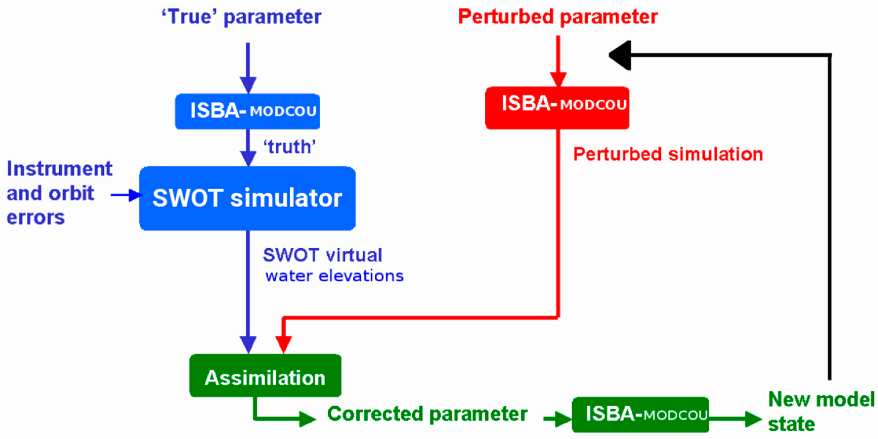
3.2. Data Assimilation Algorithm and SWOT Observing System Simulation Experiment
3.3. Sensitivity of the River Depth to the Roughness Coefficient, Kstr
3.4. Data Assimilation Experiment Setting
3.4.1. SWOT-Like Observations Generation and Their Processing
3.4.2. Description of the Variables Used in the DA Platform
3.4.3. Description of the Data Assimilation Experiments
- In a DA window, there are zero or one river depth observations: It is impossible to assimilate a δh term; and
- In a DA window, there are n observations (n ≥ 2): It is possible to assimilate n − 1 δh terms.
4. Results
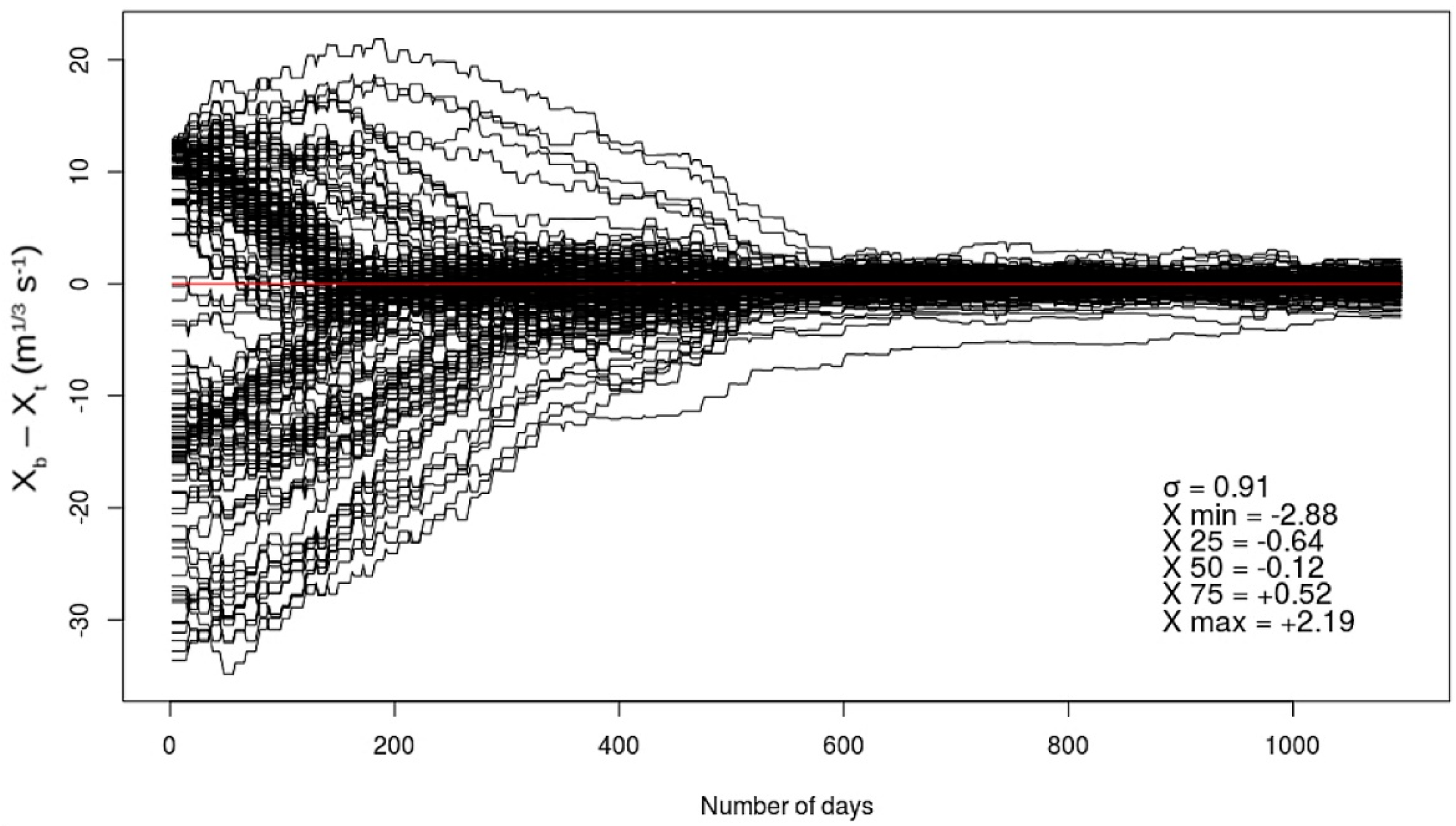
4.1. Assimilation of River Depths (Experiment 1)
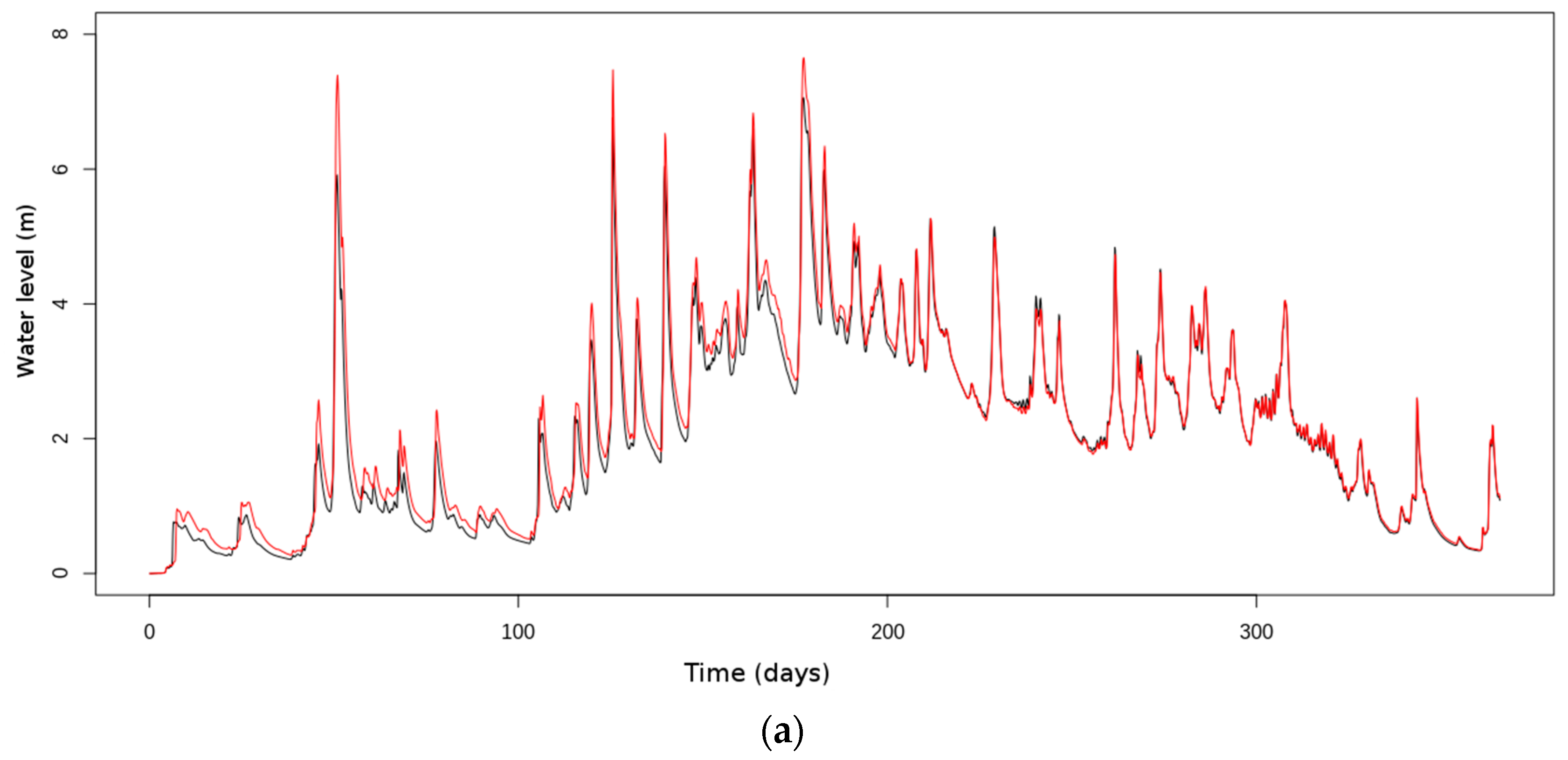
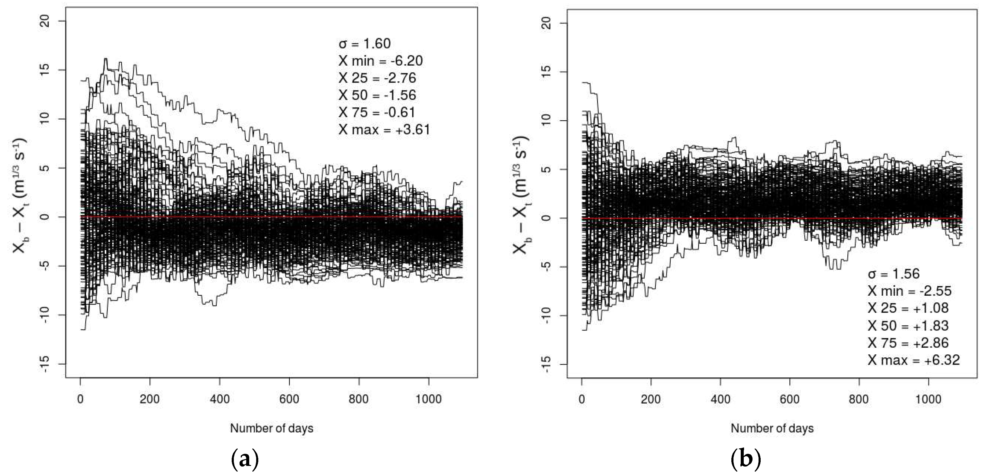
4.2. Assimilation of River Depths, in case of Atmospheric Forcing Biases (Experiment 2)
4.3. Assimilation or River Depth Differences (Experiment 3)
4.4. Assimilation of River Depths Considering More Realistic SWOT Errors (Experiment 4)
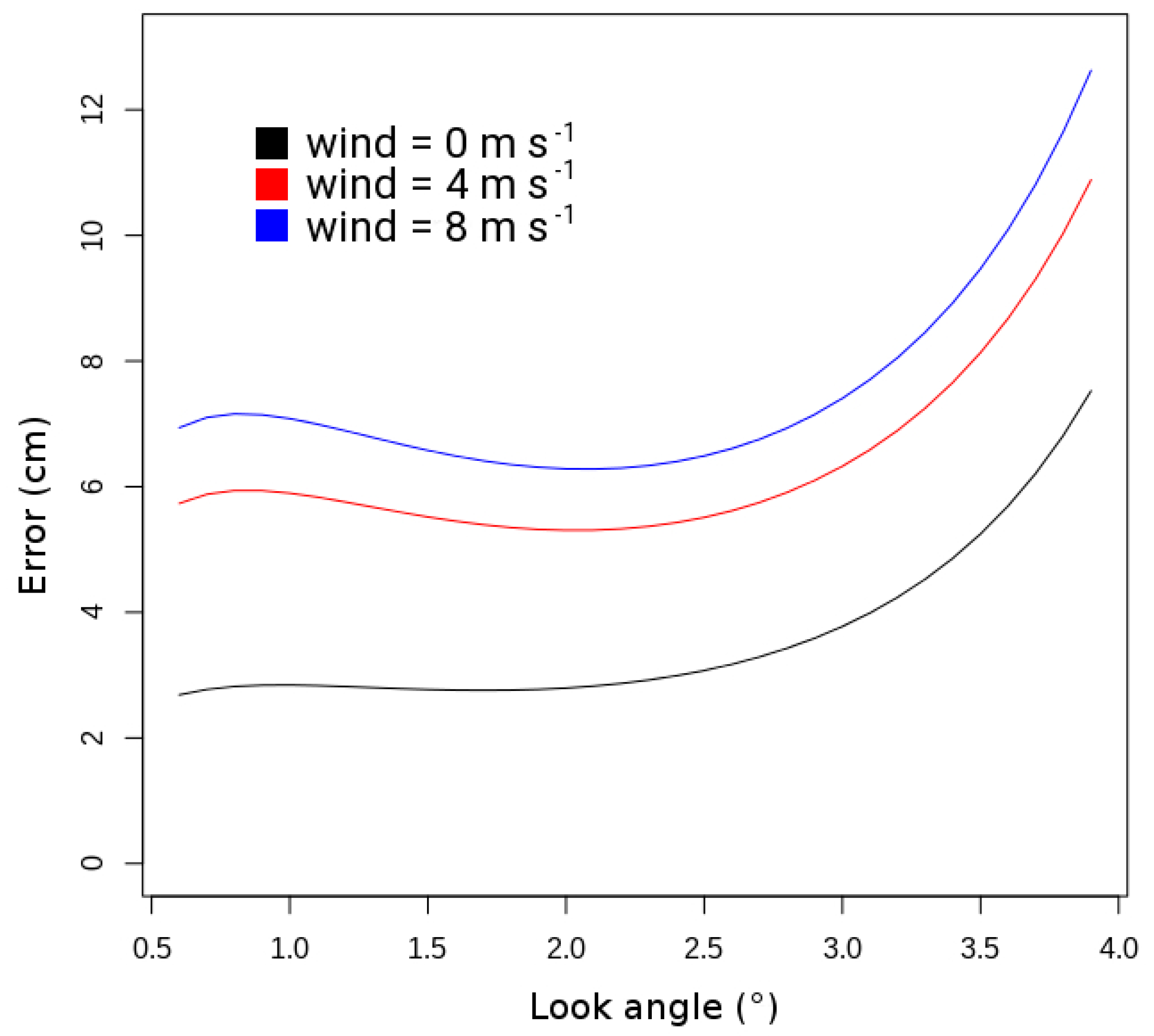
4.4.1. SWOT Instrumental Error along the Swath
4.4.2. The Intra-Day Variability of Water Content in the Troposphere: Impact on the SWOT Error of Measurement
4.4.3. SWOT DA Experiment Using Realistic Errors of Measurement
5. Conclusion and Perspectives
5.1. The Choice of the Data Assimilation Method and the Experimental Design
5.2. Choice of the Observation to Assimilate and the Parameter to Correct
5.3. Assimilation of River Depths Considering More Realistic Meteorological and SWOT Errors
5.4. Extension of SWOT DA in Other Catchments of the World
Author Contributions
Funding
Acknowledgments
Conflicts of Interest
References
- Biancamaria, S.; Lettenmaier, D.P.; Pavelsky, T.M. The SWOT mission and Its capabilities for land hydrology. Surv. Geophys. 2016, 37, 307–337. [Google Scholar] [CrossRef]
- Biancamaria, S.; Andreadis, K.M.; Durand, M.; Clark, E.A.; Rodríguez, E.; Mognard, N.M.; Alsdorf, D.E.; Lettenmaier, D.P.; Oudin, Y. Preliminary characterization of SWOT hydrology error budget and global capabilities. IEEE J. Sel. Top. Appl. Earth Obs. Remote Sens. 2010, 3, 6–19. [Google Scholar] [CrossRef]
- Bjerklie, D.M.; Lawrence Dingman, S.; Vorosmarty, C.J.; Bolster, C.H.; Congalton, R.G. Evaluating the potential for measuring river discharge from space. J. Hydrol. 2003, 278, 17–38. [Google Scholar] [CrossRef]
- Crétaux, J.F.; Jelinski, W.; Calmant, S.; Kouraev, A.; Vuglinski, V.; Berge-Nguyen, M.; Gennero, M.C.; Nino, F.; Del Rio, R.A.; Cazenave, A.; et al. SOLS: A lake database to monitor in the Near Real Time water level and storage variations from remote sensing data. Adv. Space Res. 2011, 47, 1497–1507. [Google Scholar] [CrossRef]
- Seyoum, W.M. Characterizing water storage trends and regional climate influence using GRACE observation and satellite altimetry data in the Upper Blue Nile River Basin. J. Hydrol. 2018, 556, 274–284. [Google Scholar] [CrossRef]
- Santos da Silva, J.; Calmant, S.; Seyler, F.; Corrêa Rotunno Filho, O.; Cochonneau, G.; João Mansur, W. Water levels in the Amazon basin derived from the ERS2 and ENVISAT radar altimetry missions. Remote Sens. Environ. 2010, 114, 2160–2181. [Google Scholar] [CrossRef]
- Schneider, R.; Tarpanelli, A.; Nielsen, K.; Madsen, H.; Bauer-Gottwein, P. Evaluation of multi-mode CryoSat-2 altimetry data over the Po River against in situ data and a hydrodynamic model. Adv. Water Resour. 2018, 112, 17–26. [Google Scholar] [CrossRef]
- Alsdorf, D.E.; Rodríguez, E.; Lettenmaier, D.P. Measuring surface water from space. Rev. Geophys. 2007, 45. [Google Scholar] [CrossRef]
- Pavelsky, P.; Durand, M.; Andreadis, K.M.; Beighley, R.E.; Paiva, R.C.D.; Allen, G.H.; Miller, Z.F. Assessing the potential global extent of SWOT river discharge observations. J. Hydrol. 2014, 519, 1519–1525. [Google Scholar] [CrossRef]
- Rodríguez, E.; Surface Water and Ocean Topography (SWOT). Science Requirements Document, JPL Docment D-61923. 2016. [Google Scholar]
- Zaitchik, B.F.; Rodell, M.; Reichle, R.H. Assimilation of GRACE Terrestrial Water Storage Data into a Land Surface Model: Results for the Mississippi River Basin. J. Hydrometeorol. 2008, 9, 535–548. [Google Scholar] [CrossRef]
- Biancamaria, S.; Durand, M.; Andreadis, K.M.; Bates, P.D.; Boone, A.; Mognard, N.M.; Rodríguez, E.; Alsdorf, D.E.; Lettenmaier, D.P.; Clark, E.A. Assimilation of virtual wide swath altimetry to improve Arctic river modeling. Remote Sens. Environ. 2011, 115, 373–381. [Google Scholar] [CrossRef]
- Pedinotti, V.; Ricci, S.; Biancamaria, S.; Mognard, N. Assimilation of satellite data to optimize large scale hydrological model parameters: A case study for the SWOT mission. Hydrol. Earth Syst. Sci. 2014, 18, 4485–4507. [Google Scholar] [CrossRef]
- Häfliger, V.; Martin, E.; Boone, A.; Habets, F.; David, C.H.; Garambois, P.A.; Roux, H.; Ricci, S.; Berthon, L.; Thévenin, A. Evaluation of Regional-Scale River Depth Simulations Using Various Routing Schemes within a Hydrometeorological Modeling Framework for the Preparation of the SWOT Mission. J. Hydrometeorol. 2015, 16, 1821–1842. [Google Scholar] [CrossRef]
- Caballero, Y.; Voirin-Morel, S.; Habets, F.; Noilhan, J.; Le Moigne, P.; Lehenaff, A.; Boone, A. Hydrological sensitivity of the Adour-Garonne river basin to climate change. Water Resour. Res. 2007, 43. [Google Scholar] [CrossRef]
- Noilhan, J.; Planton, S. A simple parameterization of land surface processes for meteorological models. Mon. Weather Rev. 1989, 117, 536–549. [Google Scholar] [CrossRef]
- Masson, V.; Le Moigne, P.; Martin, E.; Faroux, S.; Alias, A.; Alkama, R.; Belamari, S.; Barbu, A.; Boone, A.; Bouyssel, F.; et al. The SURFEX v7.2 land and ocean surface platform for coupled or offline simulation of earth surface variables and fluxes. Geosci. Model Dev. 2013, 6, 929–960. [Google Scholar] [CrossRef]
- Faroux, S.; Kaptué Tchuenté, A.T.; Roujean, J.-L.; Masson, V.; Martin, E.; Le Moigne, P. ECOCLIMAP-II/Europe: A twofold database of ecosystems and surface parameters at 1 km resolution based on satellite information for use in land surface. meteorological and climate models. Geosci. Model Dev. 2013, 6, 563–582. [Google Scholar] [CrossRef]
- Quintana-Seguí, P.; Le Moigne, P.; Durand, Y.; Martin, E.; Habets, F. Analysis of near-surface atmospheric variables: Validation of the SAFRAN analysis over France. Appl. Meteorol. Clim. J. 2008, 47, 92–107. [Google Scholar] [CrossRef]
- Boone, A.; Masson, V.; Meyers, T.; Noilhan, J. The influence of the inclusion of soil freezing on simulations by a soil–vegetation–atmosphere transfer scheme. Appl. Meteorol. J. 2000, 39, 1544–1569. [Google Scholar] [CrossRef]
- Decharme, B.; Boone, A.; Delire, C.; Noilhan, J. Local evaluation of the interaction between Soil Biosphere Atmosphere soil multilayer diffusion scheme using four pedotransfer functions. Geophys. Res. J. 2011, 116. [Google Scholar] [CrossRef]
- Decharme, B.; Martin, E.; Faroux, S. Reconciling soil thermal and hydrological lower boundary conditions in land surface models. Geophys. Res. Atmos. J. 2013, 118, 7819–7834. [Google Scholar] [CrossRef]
- Ledoux, E.; Girard, G.; Villeneuve, J.P. Proposition d’un modèle couplé pour la simulation conjointe des écoulements de surface et des écoulements souterrains sur un bassin hydrologique. La Houille Blanche 1984, 1–2, 101–110. [Google Scholar] [CrossRef]
- David, C.H.; Habets, F.; Maidment, D.R.; Yang, Z.-L. RAPID applied to the SIM France model. Hydrol. Proess. 2011, 25, 3412–3425. [Google Scholar] [CrossRef]
- David, C.H.; Maidment, D.R.; Niu, G.Y.; Yang, Z.L.; Habets, F.; Eijkhout, V. River network routing on the NHDPlus dataset. J. Hydrometeorol. 2011, 12, 913–934. [Google Scholar] [CrossRef]
- Farr, T.G.; Rosen, P.A.; Caro, E.; Crippen, R.; Duren, R.; Hensley, S.; Kobrick, M.; Paller, M.; Rodríguez, E.; Roth, L.; et al. The Shuttle Radar Topography Mission. Rev. Geophys. 2007, 45. [Google Scholar] [CrossRef]
- Decharme, B.; Alkama, R.; Douville, H.; Becker, M.; Cazenave, A. Global Evaluation of the ISBA−TRIP Continental Hydrological System. Part II: Uncertainties in River Routing Simulation Related to Flow Velocity and Groundwater Storage. Hydrometeorol. J. 2010, 11, 601–617. [Google Scholar] [CrossRef]
- Alkama, R. Global evaluation of the ISBA-TRIP continental hydrological system. Part I: Comparison to GRACE terrestrial water storage estimates and in situ river discharges. J. Hydrometeorol. 2010, 11, 583–600. [Google Scholar] [CrossRef]
- Pedinotti, V.; Boone, A.; Decharme, B.; Crétaux, J.F.; Mognard, N.; Panthou, G.; Papa, F.; Tanimou, B.A. Evaluation of the ISBA-TRIP continental hydrological system over the Niger basin using in situ and satellite derived datastes. Hydrol. Earth Syst. Sci. 2012, 16, 1745–1773. [Google Scholar] [CrossRef]
- Bouttier, F.; Courtier, P. Data Assimilation Concepts and Methods; ECMWF Lecture Note: Reading, UK, 1999. [Google Scholar]
- Buis, S.; Piacentini, A.; Déclat, D. PALM: A Computational framework for assembling high performance computing applications. Concurr. Comput. Pract. Exp. 2006, 18, 247–262. [Google Scholar] [CrossRef]
- Fouilloux, A.; Piacentini, A. The PALM Project: MPMD Paradigm for an Oceanic Data Assimilation Software. Comput. Sci. 1999, 1685, 1423–1430. [Google Scholar]
- Barthélémy, S.; Ricci, S.; Rochoux, M.C.; Le Pape, E.; Thual, O. Ensemble-based data assimilation for operational flood forecasting—On the merits of state estimation for 1D hydrodynamic forecasting through the example of the “Adour Marine” river. J. Hydrol. 2017, 552, 210–224. [Google Scholar] [CrossRef]
- Enjolras, V.; Vincent, P.; Souyris, J.-C.; Rodríguez, E.; Phalippou, L.; Cazenave, A. Performances study of interferometric radar altimeters: From the instrument to the global mission definition. Sensors 2006, 6, 164–192. [Google Scholar] [CrossRef]
- Brown, S.; Obligis, E. SWOT Wet Tropospheric Correction Working Group Report. In Proceedings of the 3rd SWOT Science Defintion Team Meeting, Washington, DC, USA, 14–16 January 2014. [Google Scholar]
- Fernandez, D.E. SWOT Project, Mission Performance and Error Budget, JPL Document D-79084. 2017. [Google Scholar]
- Cimini, D.; Pierdicca, N.; Pichelli, E.; Ferretti, R.; Mattioli, V.; Bonafoni, S.; Montopoli, M.; Perissin, D. On the accuracy of integrated water vapor observations and the potential for mitigating electromagnetic path delay error in InSAR. Atmos. Meas. Tech. 2012, 5, 1015–1030. [Google Scholar] [CrossRef]
- Ning, T.; Elgered, G.; Willen, U.; Johansson, J.M. Evaluation of the atmospheric water vapor content in a regional climate model using ground-based GPS measurements. J. Geophys. Res. Atmos. 2013, 118, 329–339. [Google Scholar] [CrossRef]
- Flentje, H.; Dörnbrack, A.; Fix, A.; Ehret, G.; Holm, E. Evaluation of ECMWF water vapour fields by airborne differential absorption lidar measurements: A case study between Brazil and Europe. Atmos. Chem. Phys. 2007, 7, 5033–5042. [Google Scholar] [CrossRef]
- Evensen, G. The ensemble Kalman filter: Theoritical formulation and practical implementation. Ocean Dyn. 2003, 53, 343–367. [Google Scholar] [CrossRef]
- Thirel, G.; Martin, E.; Mahfouf, J.-F.; Massart, S.; Ricci, S.; Habets, F. A past discharge assimilation system for ensemble streamflow forecasts over France—Part 1: Description and validation of the assimilation system. Hydrol. Earth Syst. Sci. 2010, 14, 1623–1637. [Google Scholar] [CrossRef]


| ΔKstr | Averaged Δh |
|---|---|
| −5% (−1.5 m1/3 s−1) | +1.5 cm |
| +5% (+1.5 m1/3 s−1) | +1.0 cm |
| −20% (−6 m1/3 s−1) | +7.5 cm |
| +20% (+6 m1/3 s−1) | +3.5 cm |
| Symbol | Variable | Dimension |
|---|---|---|
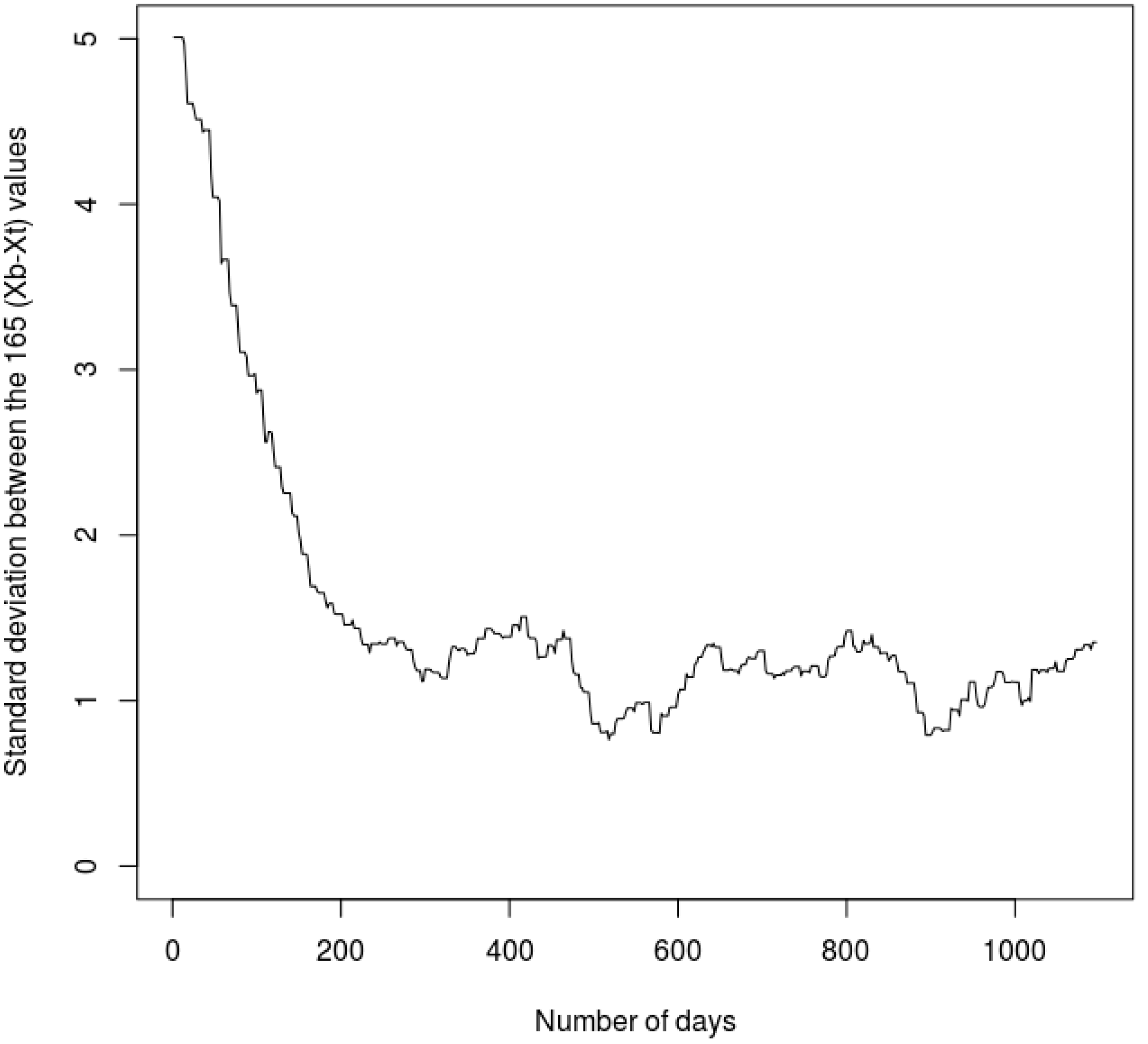
| xb | A priori vector of the Strickler coefficients | 165 |
| xt | Truth vector of the Strickler coefficients | 165 |
| xa | Analysis vector of the Strickler coefficients | 165 |
| yo | Observation vector of the synthetic SWOT river depths during a DA window | p |
| H(xb) | Model equivalent of the yo vector, with the river depths simulated by RAPID during a DA window | p |
| R | Observation error matrix of river depths | p × p |
| B | Model error matrix of Strickler coefficients | 165 × 165 |
| H | Jacobian matrix: sensitivity of H(xb) to a perturbation of the Strickler coefficient in the model | 165 × p |
| Criterion | Experiment 1: River Depth Assimilation | Experiment 2: River Depth Assimilation by Perturbing ISBA Outputs | Experiment 3: Difference of River Depth Assimilation | Experiment 4: River Depth Assimilation Considering More Realistic SWOT Errors |
|---|---|---|---|---|
| Assimilation type | River depths | River depths; ISBA runoff and drainage perturbed ±10% | river depth differences | River depths |
| Window duration | 48 h | 48 h | 42 days | 48 h |
| Beginning of the experiment | 1 August 1995 | 1 August 1995 | 1 August 1995 | 1 August 1995 |
| End of the experiment | 31 July 1998 | 31 July 1998 | 15 April 2001 | 31 July 1998 |
| First a priori value xb | Each value of Strickler coefficient are equal to 25 m1/3 s−1 | “Truth” of the 165 Strickler coefficient values perturbed with a centered Gaussian noise, σxb, equal to 5 m1/3 s−1 | “Truth” of the 165 Strickler coefficient values perturbed with a centered Gaussian noise, σxb, equal to 5 m1/3 s−1 | “Truth” of the 165 Strickler coefficient values perturbed with a centered Gaussian noise, σxb, equal to 5 m1/3 s−1 |
| Definition of the matrix B | Diagonal, each value σB2 is equal to the variance of all the xb values around the truth. Minimum imposed value = (1.5 m1/3 s−1)² | Diagonal, each value σB2 is equal to the variance of all the xb values around the truth. Minimum imposed value = (1.5 m1/3 s−1)² | Diagonal, each value σB2 is equal to the variance of all the xb values around the truth. Minimum imposed value = (2.12 m1/3 s−1)² | Diagonal, each value σB2 is equal to the variance of all the xb values around the truth. Minimum imposed value = (1.5 m1/3 s−1)² |
| Definition of the matrix R | Diagonal, each value σR2 is equal to (10 cm)² | Diagonal, each value σR2 is equal to (10 cm)² | Diagonal, each value σR2 is equal to (10 cm)² | Diagonal, each value σR2 varies in the time and the space |
| Hydrology Error Component | Height Error (cm) |
|---|---|
| Ionosphere signal (constant) | 0.80 |
| Dry troposphere signal (constant) | 0.70 |
| Wet troposphere signal (variable) | 4.00 |
| Orbit radial component (constant) | 1.62 |
| KaRIn Random and systematic errors after cross-over correction (constant) | 7.74 |
| Surface of the reach + look angle + wind speed (variable) | 4.40 |
| Total allocation | 9.95 |
| Unallocated margin (constant) | 1.04 |
| Total error | 10.0 |
© 2019 by the authors. Licensee MDPI, Basel, Switzerland. This article is an open access article distributed under the terms and conditions of the Creative Commons Attribution (CC BY) license (http://creativecommons.org/licenses/by/4.0/).
Share and Cite
Häfliger, V.; Martin, E.; Boone, A.; Ricci, S.; Biancamaria, S. Assimilation of Synthetic SWOT River Depths in a Regional Hydrometeorological Model. Water 2019, 11, 78. https://doi.org/10.3390/w11010078
Häfliger V, Martin E, Boone A, Ricci S, Biancamaria S. Assimilation of Synthetic SWOT River Depths in a Regional Hydrometeorological Model. Water. 2019; 11(1):78. https://doi.org/10.3390/w11010078
Chicago/Turabian StyleHäfliger, Vincent, Eric Martin, Aaron Boone, Sophie Ricci, and Sylvain Biancamaria. 2019. "Assimilation of Synthetic SWOT River Depths in a Regional Hydrometeorological Model" Water 11, no. 1: 78. https://doi.org/10.3390/w11010078
APA StyleHäfliger, V., Martin, E., Boone, A., Ricci, S., & Biancamaria, S. (2019). Assimilation of Synthetic SWOT River Depths in a Regional Hydrometeorological Model. Water, 11(1), 78. https://doi.org/10.3390/w11010078