Numerical Study of the Velocity Decay of Offset Jet in a Narrow and Deep Pool

Abstract

The present study examines the configuration of an offset jet issuing into a narrow and deep pool. The standard k-ε model with volume-of-fluid (VOF) method was used to simulate the offset jet for three exit offset ratios (OR = 1, 2 and 3), three expansion ratios (ER = 3, 4 and 4.8), and different jet exits (circular and rectangular). The results clearly show significant effects of the circumference of jet exits (L_exit) in the early region of flow development, and a fitted formula is presented to estimate the length of the potential core zone (L_PC). Analysis of the flow field for OR = 1 showed that the decay of cross-sectional streamwise maximum mean velocity (U_m) in the transition zone could be fitted by power law with the decay rate n decreased from 1.768 to 1.197 as the ER increased, while the decay of U_m for OR = 2 or 3 was observed accurately estimated by linear fit. Analysis of the flow field of circular offset jet showed that U_m for OR = 2 decayed fastest due to the fact that the main flow could be spread evenly in floor-normal direction. For circular jets, the offset ratio and expansion ratio do not affect the spread of streamwise velocity in the early region of flow development. It was also observed that the absence of sudden expansion of offset jet is analogous to that of a plane offset jet, and the flow pattern is different.

1. Introduction

Offset jets are common in drainage systems [1], slot fishways [2], and hydraulics engineering [3]. The offset jet is formed when a fluid jet discharges into an ambient medium above the floor and parallel to the axis of the jet exit but which is offset by a certain height. The submerged offset jets in the narrow and deep pool are more complex flow because it can easily be affected by side walls.

The offset jet flow was widely used as energy dissipation downstream of hydraulic structures—for example, the submerged hydraulic jump at an abrupt drop could be considered as an offset jet flow. From an engineering point-of-view, the length of the stilling basin should be as short as possible. The focus of this paper is to find the factors affect the efficiency of energy dissipation of the offset jet flow. Figure 1 shows a sketch of the submerged offset jet in a pool. The jet is mainly divided into three regions according to the relationship with the floor, viz., recirculation region, impingement region, and wall jet region. The Cartesian coordinate system is used with x, y, and z representing the streamwise, lateral direction, and floor-normal direction, respectively. The exit of the jet is at x = 0, and the symmetry plane is at y = 0, the pool bottom is at z = 0. The symbols L_x, L_y, L_z, S, d, h_t, U_j, and U_m represent the length, width, and height of jet pool, offset height, the diameter of jet exit, depth of tailwater, bulk velocity, and cross-sectional streamwise maximum mean velocity, respectively. Likewise, if the jet exit is rectangular, a₀, b₀ represents the height and width of the rectangle, respectively. The flow field in jet pool can be divided into three zones by the decay of U_m: (a) the potential core zone, where U_m was equal to the jet exit velocity, U_j; (b) transition zone, where the decay of U_m was rapidly in this zone; and (c) fully development zone, where the decay of U_m became very slow.

The recent studies on submerged offset jets were carried out by Subhasish Dey [4] to investigate the vertical profiles of time-averaged velocity components, and Reynolds stresses in jet flows for offset ratios OR = 2.8–5.1, submergence ratio SR = 2.4–5.6, expansion ratio ER = 1, and jet Reynold number R₀ = 28,475–80,730, where OR = S/a₀ (for circular jet exit a₀ = d), SR = h_t/S, ER = L_y/b₀, and R₀ = (U₀a₀)/υ, υ is the coefficient of kinematic viscosity of water. They concluded important characteristic length of submerged offset jets, such as the length of the recirculation region and impingement region, are expressed as a function of the R₀, OR, and SR. In another attempt, Bhuiyan [5] analyzed the characteristics of submerged turbulent plane offset jets (OR = 0.5–3.6) in channels with rough beds and shallow tailwater depths. The results indicated that for an offset height larger than the jet thickness, the peak velocity, the flow momentum decay faster in the downstream direction in an offset jet than in a turbulent plane wall jet. Durand et al. [6] studied the effect of Reynolds number on 3D offset jets both experimentally and numerically for R₀ = 34,000, 53,000 and 86,000. The results indicated the floor-normal location of maximum mean velocity and jet spread to be independent of Reynolds number. The investigated by Nyantekyi-Kwakye [7] on a 3D rectangular offset jet, performed at three offset ratios (OR = 0, 2, and 4) and revealed that large-scale structures dominate the inner layer of the wall jet region. For 3D circular offset jets (with OR ranging from 0–3.5), Agelin-chaab and Tachie [8] using a planar particle image velocimetry (PIV) system conducted the experiments to study the velocity. They observed that OR influenced both the decay of U_m and growth of the shear layer within the developing region. Besides, there have been other experimental studies on 3D offset jets [9,10,11].

Given the brief overview, it can be concluded that the mechanics of offset jet has been studied extensively. However, the hydraulic properties of submerged offset jets in a narrow and deep pool have not been completely understood, although it was widely used as an efficient energy dissipator in hydraulic engineering located in narrow canyons.

This paper addresses the decay of velocity of offset jets in the narrow and deep pool with various offset ratios, expansion ratios and jet exit shapes, through numerical simulations using a 3D computational fluid dynamics (CFD) model with the k-ε turbulence model coupled with VOF method, which was confirmed perform well in jet flow [10,12,13,14,15,16,17].

2. Numerical Simulation

2.1. Mathematical Model

An RNG k-ε model has been compared to a standard k-ε model for computing transient jets by Abraham and Maji [18] and concluded that the RNG k-ε model results in predictions of greater mixing in the jets relative to the standard model. The study carried by Nasr and Lai [19] indicated that the standard k-ε turbulence model predicts better than RNG k-ε and Reynolds stress turbulence model. In this study, the standard k-ε model [20] was used as the turbulence closure

$$\frac{\partial \left(\rho k\right)}{\partial t}+\frac{\partial \left(\rho u_{i}k\right)}{\partial x_i}=\frac{\partial }{\partial x_i}\left[\left(\mu +\frac{{\mu }_t}{{\sigma }_k}\right)\frac{\partial k}{\partial x_i}\right]+G_k-\rho \epsilon$$

(1)

$$\frac{\partial \left(\rho \epsilon \right)}{\partial t}+\frac{\partial \left(\rho u_i\epsilon \right)}{\partial x_i}=\frac{\partial }{\partial x_i}\left[\left(\mu +\frac{{\mu }_t}{{\sigma }_{\epsilon }}\right)\frac{\partial \epsilon }{\partial x_i}\right]+C_{1\epsilon }\frac{\epsilon }{k}{G}_k-C_{2\epsilon }\rho \frac{{\epsilon }^2}{k}$$

(2)

where $\rho$ is the density of mixture; t is time; k is turbulent kinetic energy; $\mu$ is the dynamic viscosity of fluid; u_i is component of velocity in the x_i direction; $\epsilon$ is turbulent energy dissipation rate; ${\mu }_t$ is dynamic turbulent viscosity; ${\sigma }_k$, ${\sigma }_{\epsilon }$ is turbulent Prandtl number for k and $\epsilon$, respectively; $G_k$ is generation of turbulent kinetic energy due to mean velocity gradients; and ${\mu }_t$ and $G_k$ can be determined as

$${\mu }_t=\rho C_{\mu }\frac{k^2}{\epsilon }$$

(3)

$$G_k={\mu }_t\left(\frac{\partial u_i}{\partial x_j}+\frac{\partial u_j}{\partial x_i}\right)\frac{\partial u_i}{\partial x_j}$$

(4)

The values of the empirical constants in the turbulence model are $C_{\mu }=0.09$, ${\sigma }_k=1.0$, ${\sigma }_{\epsilon }=1.3$, $C_{1\epsilon }=1.44$, and $C_{2\epsilon }=1.92$.

For this study, the volume-of-fluid (VOF) method was used as the two-phase flow model to track the water surface in the domain. The VOF method is widely used to determine the position of the interface of two or more immiscible flows [21,22]. Air and water were the primary and secondary phases, respectively. In the calculation, all fluids share the turbulence model. For air-water two-phase flow, ${\alpha }_a$ and ${\alpha }_w$ are the volume fraction of air and water, respectively. For each control cell,

$${\alpha }_w+{\alpha }_a=1$$

(5)

If the cell contains only air, the value of ${\alpha }_w$ = 0; if the cell is full of water, the value of ${\alpha }_w$ = 1; and if the interface cuts the cell, then $0<{\alpha }_w<1$. The volume fraction of water, ${\alpha }_w$, is calculated from [23]

$$\frac{\partial {\alpha }_w}{\partial t}+V·\nabla {\alpha }_w=0$$

(6)

where the $V$ is the fluid velocity. The fluid properties, such as density $\rho$ and molecular viscosity $\mu$, are adjusted according to the volume fraction. It should be noted that other numerical methods can also be used to study the detailed flow properties in complex contexts [24,25,26,27,28,29], the choice of numerical methods depends on the research focus.

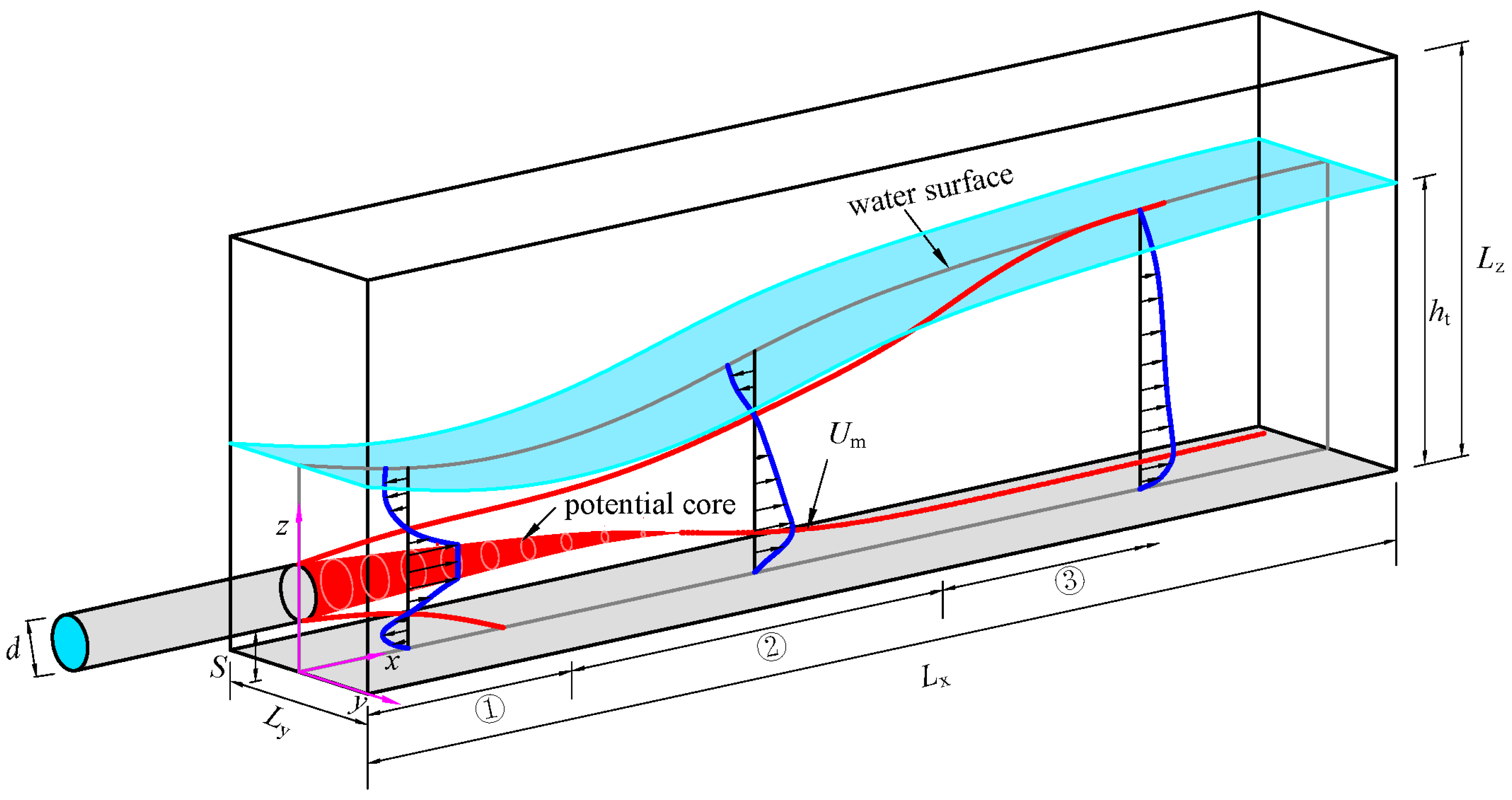
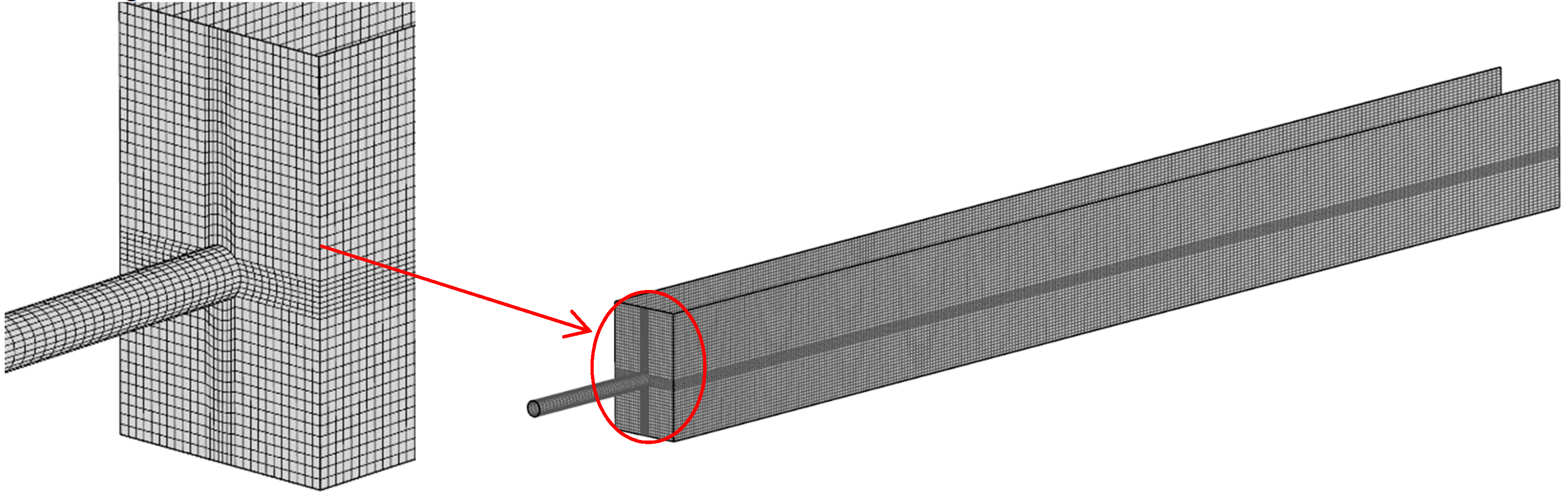
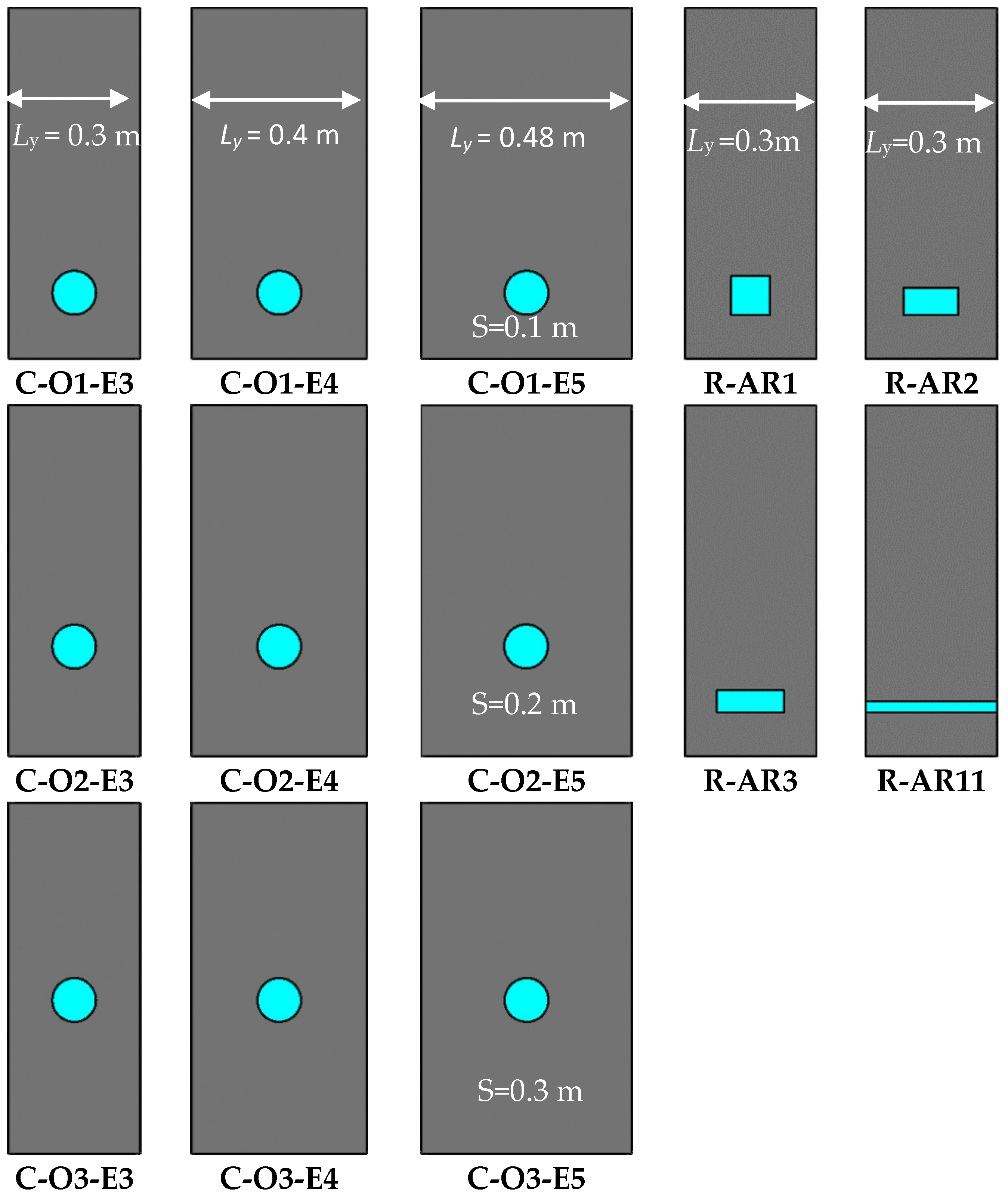
2.2. Simulation Setup

ANSYS ICEM 16.0 (ANSYS^®, Canonsburg, PA, USA) was utilized to develop the numerical models for 13 types of offset jet. Hexahedral grids were used throughout the computational domain. The grid meshing is shown in Figure 2. A Cartesian coordinate system is used so that the origin is at the center of the intersection of the offset wall and floor. The computational domain consists of the pipe and jet pool. The jet is discharged from offset wall offset by a height S above the floor. The total pipe length is 1 m, and the type of pipe can be divided into the circular pipe and rectangular pipe. The length, L_x, and height, L_z, of the pool are 8 m and 0.8 m, respectively. For the circular pipe, the offset ratio (OR) varied from 1 to 3, the expansion ratio (ER) varied from 3 to 4.8 as the width of the jet pool increased from 0.3 m to 0.48 m. For the rectangular pipe, the aspect ratio (AR) of the exit varied from 0.33 to 11.46. Moreover, the area of exit remains constant for all shape of exits. The parameters of all cases are given in

Table 1. Parameters of computational cases.

Case Name	Jet Exit Shape	d (m)	a0 (m)	b0 (m)	S (m)	Ly (m)	Offset Ratio (OR)	Expansion Ratio (ER)	AR (b0/a0)
C-O1-E3	circular	0.1	-	-	0.1	0.3	1	3	-
C-O1-E4	circular	0.1	-	-	0.1	0.4	1	4	-
C-O1-E5	circular	0.1	-	-	0.1	0.48	1	4.8	-
C-O2-E3	circular	0.1	-	-	0.2	0.3	2	3	-
C-O2-E4	circular	0.1	-	-	0.2	0.4	2	4	-
C-O2-E5	circular	0.1	-	-	0.2	0.48	2	4.8	-
C-O3-E3	circular	0.1	-	-	0.3	0.3	3	3	-
C-O3-E4	circular	0.1	-	-	0.3	0.4	3	4	-
C-O3-E5	circular	0.1	-	-	0.3	0.48	3	4.8	-
R-AR1	rectangular	-	0.089	0.089	0.1	0.3	1.13	3.39	1
R-AR2	rectangular	-	0.125	0.063	0.1	0.3	1.60	2.39	2
R-AR3	rectangular	-	0.153	0.051	0.1	0.3	1.95	1.95	3
R-AR11	rectangular	-	0.1	0.026	0.1	0.3	3.82	1.00	11.46

, and the jet exits and the offset wall are shown in Figure 3.

2.3. Initial Conditions and Boundary Conditions

All the variables except at boundaries (such as u_i, P, k, and ε) are initialized at zero. The computed data are stored at every alternate time step for post-processing. All computations are conducted on an Inter core i7 3.60 GHz Windows machine.

The boundary conditions were set as follows.

• Inflow boundary: the inlet was treated as an inlet velocity boundary with the velocity was set as 5 m/s;
• Outflow boundary: pressure outlet boundary was selected at the outlet, the depth of tailwater was fixed at 0.55 m with the help of user-defined function (UDF);
• Free surface: pressure inlet was employed, and its value was the standard atmospheric pressure, the operating pressure and density were selected as 101,325 Pa and 1.225 kg/m³, respectively.
• Wall boundary: for the parameters investigated in this study, the data near the wall was ineffective. No slip boundary condition is considered for velocity. To avoid the fine mesh required to resolve the viscous sub-layer near the boundary, so standard wall function method has been used.

2.4. Numerical Discretizations

ANSYS Fluent 16.0 (ANSYS^®, Canonsburg, PA, USA) was utilized to perform the simulation. The governing equations are discretized using the implicit Finite Volume Method (FVM). The SIMPLE algorithm, using a relationship between velocity and pressure corrections to enforce mass conservation and to obtain the pressure field, was applied to couple the velocity and pressure. The least-squares cell-based method was used to calculate the gradient. PRESTO! was used to discretize the pressure and Geo-Reconstruct was used for the volume fraction. The second-order upwind scheme was used for the momentum and the first-order upwind for the turbulent kinetic energy and the dissipation rate with ANSYS Fluent’s default under relaxation values for all parameters. The time step was Δt = 0.0001~0.001 s and the iteration number was always less than 2.

The computational results are considered to be converged when the residual becomes smaller than 0.001 for all equations. Here, the residual is defined as the square root of the summation of the squares of the difference between right and lefts sides of the discretized equations for a single control volume [30]. The results analyzed and presented in this study were taken from the simulation when quasi-steady state was reached.

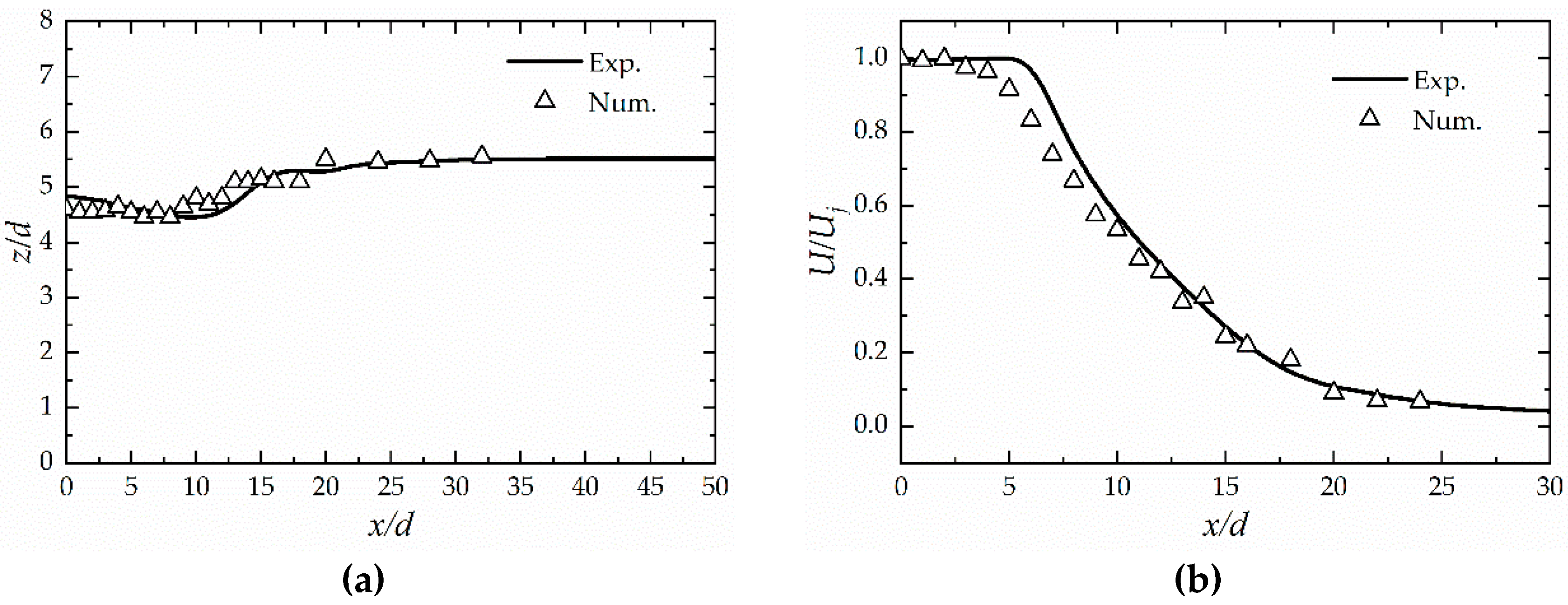
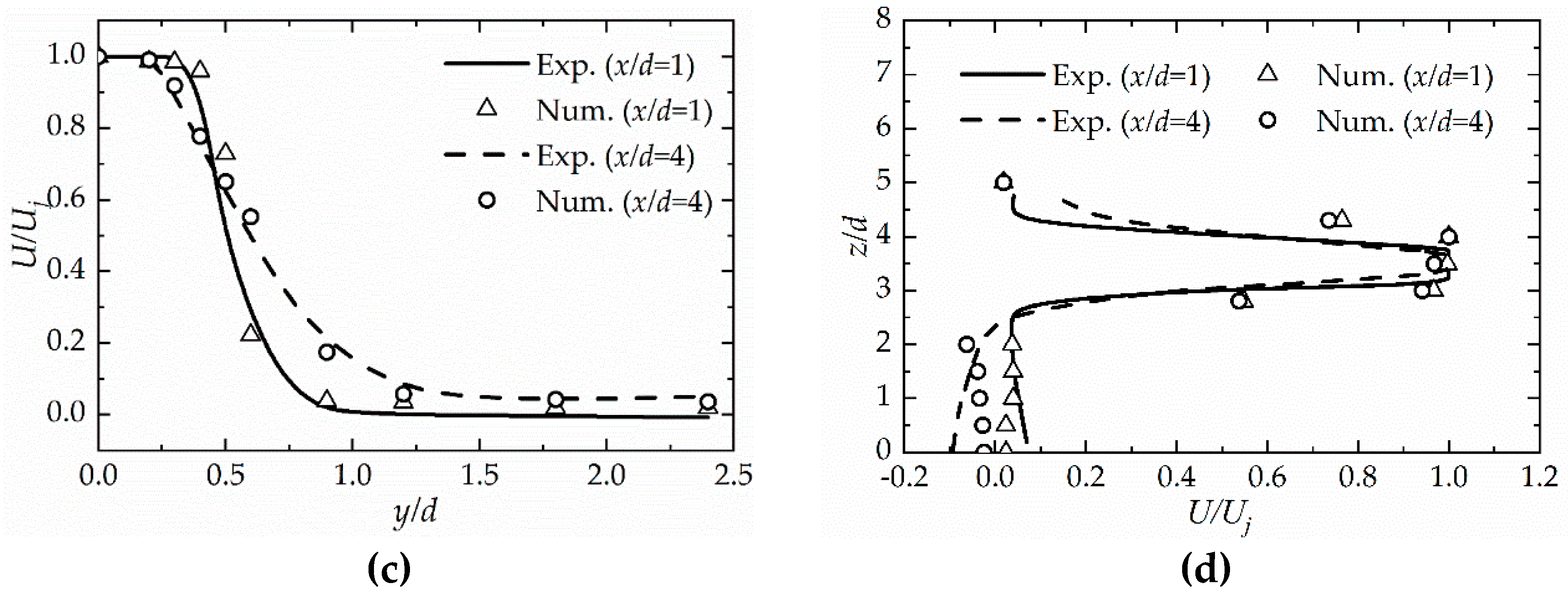
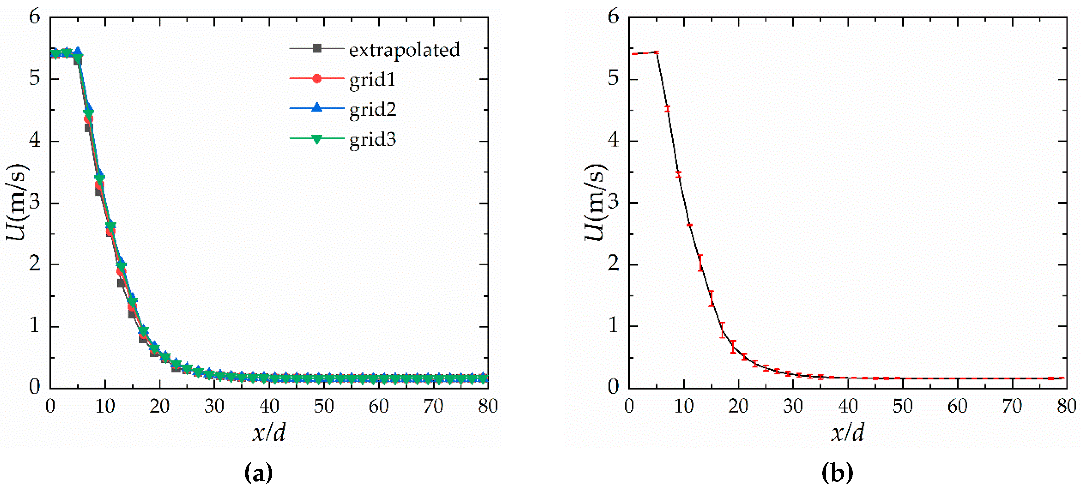
2.5. Grids Sensitivity and Model Validation

Grid independence was examined to ensure the reliability of the numerical simulation results. The Case C-O3-E5 was chosen to test mesh sensitivity. Three sets of grids had 1,065,575 (grid 1), 438,221 (grid 2) and 181,036 (grid 3) cells, respectively. The grid convergence index (GCI) is widely used to estimate discretization uncertainty [31]. The GCI is given by

$$GCI=\frac{1.25\left|\left({\varnothing }_3-{\varnothing }_2\right)/{\varnothing }_3\right|}{{\left(h_2/h_3\right)}^P-1}$$

(7)

$$P=\frac{1}{\ln \left(h_2/h_3\right)}\left|\ln \left|\left({\varnothing }_1-{\varnothing }_3\right)/\left({\varnothing }_2-{\varnothing }_3\right)\right|+\ln \left|\frac{{\left(h_2/h_3\right)}^P-\mathrm{sgn}\left[\left({\varnothing }_2-{\varnothing }_3\right)/\left({\varnothing }_2-{\varnothing }_3\right)\right]}{{\left(h_1/h_2\right)}^P-\mathrm{sgn}\left[\left({\varnothing }_1-{\varnothing }_3\right)/\left({\varnothing }_2-{\varnothing }_3\right)\right]}\right|\right|$$

(8)

where ${\varnothing }_i$ is the solution on the ith grid and h_i is the average grid size on the ith grid and h₁ > h₂ > h₃.

Figure 4 presents an axial velocity profile along the jet exit axis. In this figure, 80% out of 40 points exhibited oscillatory convergence. The maximum uncertainties in velocity were approximately 12.6%, which corresponds to a maximum uncertainty in velocity of about ±0.25 m/s. Considering the simulation accuracy and the computation efficiency, the final grid number in this study was taken as 438,221.

To examine simulation accuracy, the physical model experiment of Case C-O3-E5 was performed at the State Key Laboratory of Hydraulics and Mountain River Engineering, Sichuan University, Chengdu. The experimental model is shown in Figure 5. It can be seen from Figure 6 that the calculated results of the height of water surface and velocity distribution were fairly consistent with that of laboratory tests. The results are indicating that the numerical simulation produced reliable and acceptable results.

3. Results and Analysis

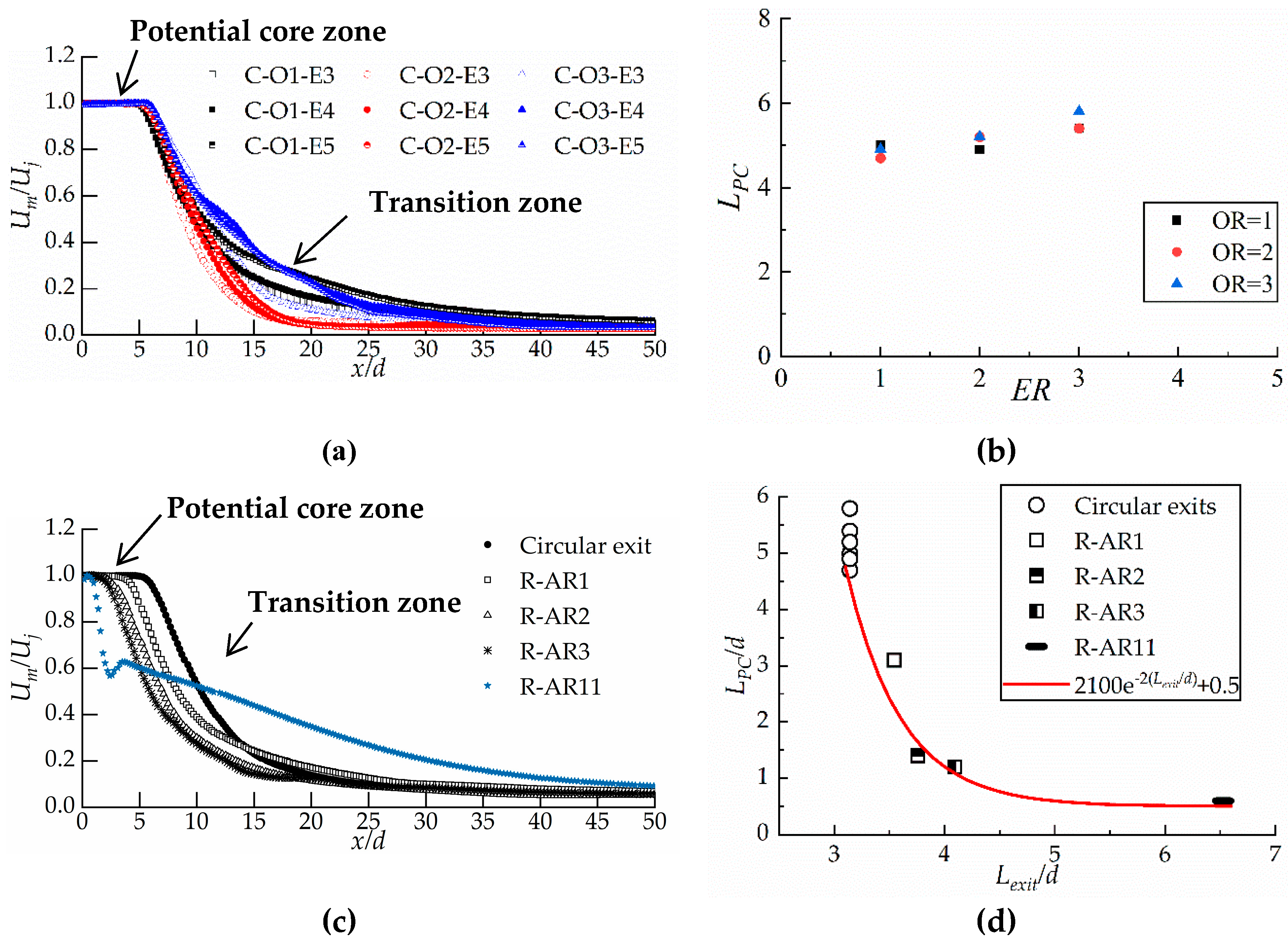
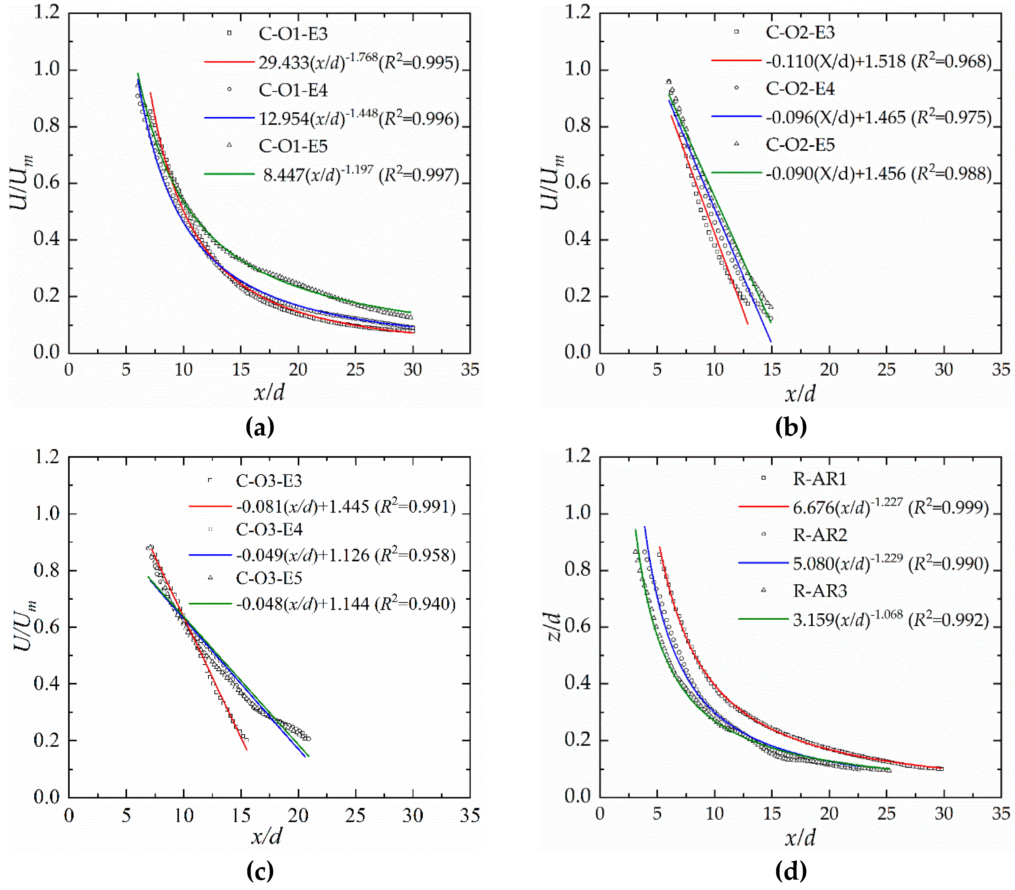
3.1. Velocity Attenuation

The attenuation of the jet flow in the narrow and deep pool was characterized using the decay of the cross-sectional maximum streamwise mean velocity (U_m). Previous studies indicated that U_m is constant within the potential core region, followed by a rapid decay with streamwise distance in transition zone [32,33]. The entrained ambient fluid gets momentum since the jet enters the pool, the section of jet flow continues to expand, and the velocity is decreasing as the results of the mixing of jet and ambient fluid. Figure 7a shows the distribution of U_m normalized by the jet exit velocity, U_j. Normalized values of U_m were observed decayed sharply within the region x/d > L_PC and the trend of decay of U_m varies greatly in the transition zone for different circular offset jet. It can be seen from Figure 7b that the length of the potential core zone (L_PC) varied from 5.0 to 5.5 with changes in ER, and a higher ER indicated a higher L_PC.

As can be observed in Figure 7c–d, the L_PC varies greatly with AR of the rectangular jet exit due to the circumference of exit (L_exit) were changed. When L_exit increased, the L_PC decreased sharply, a fitting formula was used to estimate the relationship of L_exit and L_PC as indicated in Figure 7d, the empirical equation for L_PC was employed as $L_{PC}/d=2100{\mathrm{e}}^{-2\left(L_{exit}/d\right)}+0.5$.

The decay of the U_m over distance x (scaled by d) for Case R-AR11 is shown in Figure 7c. The most striking feature of Case R-AR11 is that there is no sudden expansion (ER = 1). Thus, the Case R-AR11 is analogous to that of a plane offset jet. The decay of U_m in the recirculation region is quite sharp, the U_m drops to a local minimum value due to an increase in pressure resulting from the jet impingement after the reattachment of the jet. The decay of U_m is rather gradual in the wall jet region. A similar observation was reported by Gu [16] and Dey [4].

The U_m/U_j decay profiles can be grouped based on their characteristics. The power law of the form $U_m/U_j=C{\left(x/d\right)}^{-n}$ is typically used to describe the velocity decay in the transition zone [6,32,34,35], where C and n are a proportionality symbol and decay rate, respectively. The decay rate indicated the extent of entrainment and boundary effects on the jet. Figure 8 shows the variation of U_m/U_j for all cases with the normalized longitudinal coordinate x/d within the transition zone. Rajaratman reported n = 0.5 for a plane free jet by considering simplified conservation laws and entrainment hypotheses [36]. The wall jet was observed to be accurately estimated by using the power law. However, the distribution of U_m/U_j for the offset jets are not accurately described by the power law, which should be replaced by a linear fit [32].

For circular offset jet, using the power law fit, the decay rate for the lower offset ratio (OR = 1) circular jet was observed to be accurately estimated with the decay rate n varies from 1.197 to 1.768 as shown in Figure 8a. As can be seen in Figure 8b–c, the distributions of U_m/U_j, for the higher offset ratio (OR = 2 or 3) circular jet are not accurately described by the power law. Therefore, a linear fit was used to estimate the decay rates for higher offset ratio jet, the slope κ the linear equation was considered as the decay rate. Decay rate κ values of 0.110, 0.096 and 0.090 with R² above 0.94 were obtained for ER = 3, 4 and 4.8, respectively, when OR = 2. Decay rate values of 0.081, 0.048 and 0.049 with R² above 0.968 were obtained for ER = 3, 4 and 4.8, respectively, when OR = 3. Above analysis and as shown in Figure 8a–c indicated that when the offset ratio is moderate (OR = 2) produces a faster decay than that of higher or lower offset ratio (OR = 1 or 3). The reason is that two circulating vortices were developed below and above jet, respectively. The circulating vortices develop reverse flows against the inflow-jet direction. Negative momentum of the reverse flows reduced the inflow momentum slowing the jet rapidly down.

The decay rates for the various circular jet cases are reported in

Table 2. The decay rate of the circular jet.

Decay Rate	n (OR = 1)	κ (OR = 2)	κ (OR = 3)
Fit Equation	Power Law	Linear Equation
ER = 3	1.768	0.110	0.081
ER = 4	1.448	0.096	0.049
ER = 4.8	1.197	0.090	0.048

. The decay rate value is the largest as the expansion ratio (ER) is 3. There is a stronger jet interaction with the ambient fluid due to the more confined environment.

For rectangular offset jet, the U_m/U_j for 1 ≤ AR ≤ 3 is expressed well by power law form with the decay rate n varies from 1.068 to 1.228 (

Table 3. The decay rate of the rectangular jet.

Decay Rate	n (OR = 1)
Fit Equation	Power Law
AR = 1	1.227
AR = 2	1.229
AR = 3	1.068

), and the U_m decay in transition zone does not show substantial differences (Figure 8d). Therefore, it appears reasonable to assume the effect of the aspect ratio of the rectangular jet on the mainstream attenuation is mainly to influence the length of the potential core zone.

The algorithm for calculating the length of the potential core (L_PC) and decay profiles in the transition zone could be used to roughly calculate the length of the energy dissipation region (L_ED). For example, a square offset jet is issued to a pool. The side length of the square is 2.67 m (equivalent diameter is 3 m), the offset height is 3 m, the width of the pool is 12 m, and the height of tail water is 16.5 m. If the U/U_m = 0.2 as the end of the length of the energy dissipation region, the distance U/U_m decreases from 1 to 0.2 is called L_tr. The L_PC can be described by:

$$L_{ED}=L_{PC}+L_{tr}$$

(9)

The L_PC = 6.60 m calculated by $L_{PC}/d=2100{\mathrm{e}}^{-2\left(L_{exit}/d\right)}+0.5$. The L_tr = 39.53 m calculated by $0.2=-0.096\left(x/d\right)+1.465$. As the result, the length of energy dissipation region is 43.13 m.

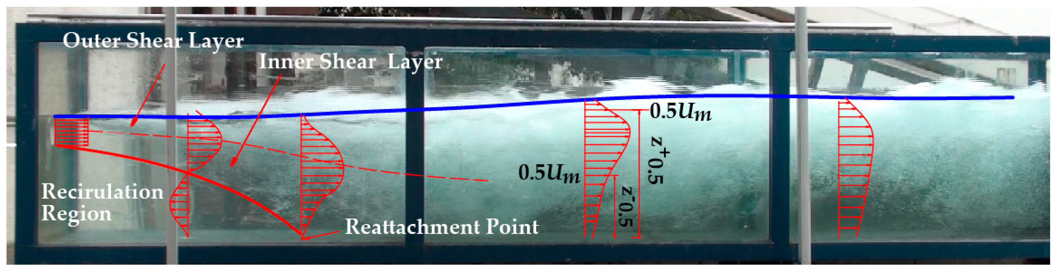
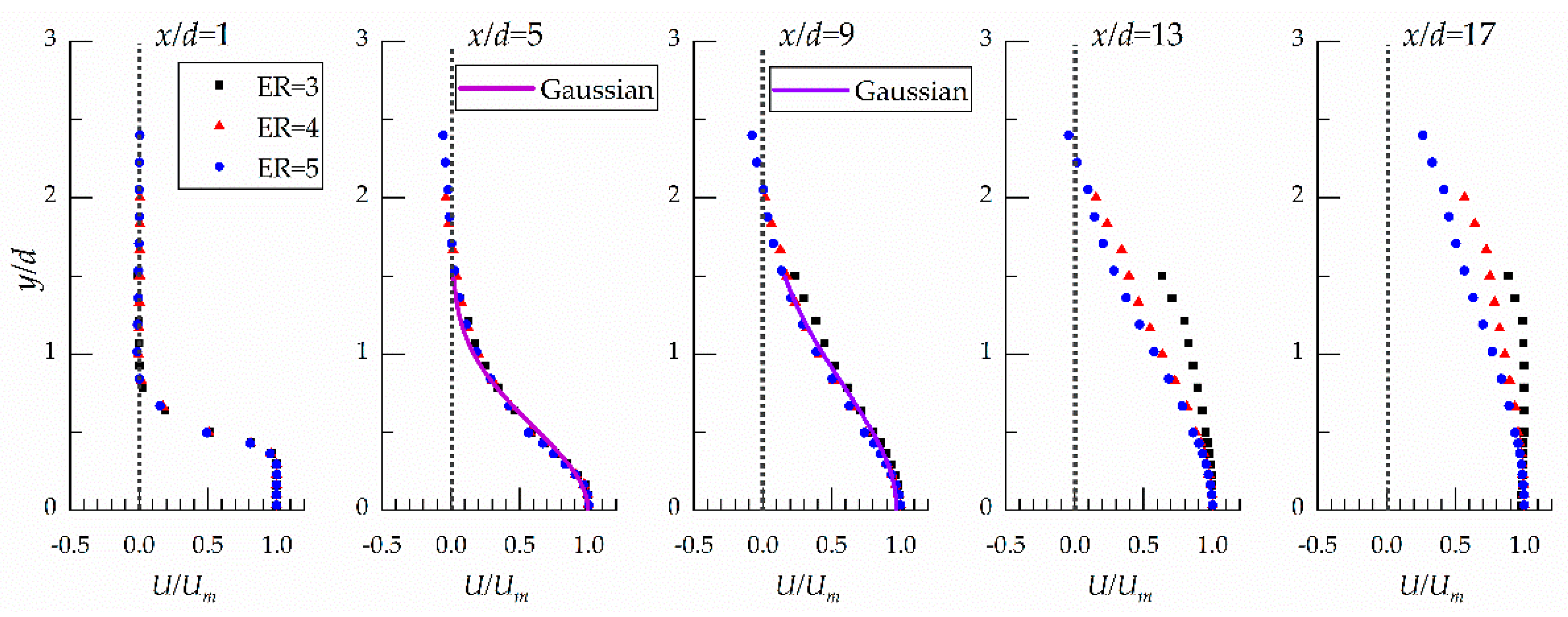
3.2. Vertical Velocity Spread

Figure 9 shows the flow field of the offset jet with different offset ratios. There is a large range of vortices formed near the jet flow, the location and size of the vortex on the streamwise section have notable differences. When OR = 1, in the range of x/d = 0–25, a large vortex was formed above the jet flow; When OR = 3, in the range of x/d = 0–25, a large vortex was formed below the jet flow. However, there is a smaller vortex above and below the jet flow in the range of x/d = 0–15.

Profiles of the streamwise mean velocities (U) extracted at x/d = 1, 4, 9, 13 and 17 are shown in Figure 10. It may be noted that to cover a range of ER = 4, Cases C-O1-E4, C-O2-E4, and C-O3-E4 were selected; otherwise, using the data of all Cases would make the plots clumsy. The velocity and length scale used was U_m and d, respectively. Here, z_c is the distance from the center of exit to the floor, that is, z − z_c = 0, where is the axis of the jet exits. Vertical profiles of U are shown in Figure 10a for ER is 4. The effect of offset ratio (OR) on the vertical velocity spread was not evident within the region x/d < 9. It can be noted that the velocity distribution in the floor-normal direction conforms with the Gaussian distribution within the region of 5 ≤ x/d ≤ 9. However, as the jet travels away from the jet exits (x/d > 9), the data of jets at different offset height are no longer overlapped. The location of the maximum of U/U_m for OR = 2 is almost at the axis of the jet exits. The location of the maximum of U/U_m is above and below the axis of the jet exits for OR = 3 and OR = 1, respectively. The results reveal offset height changes travel direction of the bulk of the jet.

Figure 10b shows the development of the U of the offset jet with rectangular exits. The results demonstrate that the bulk of the jet turns travel direction and then attaches to the floor within the region of x/d < 13. Further, the figure shows the spread rate of U is larger as the aspect ratio increases, and the flow direction for AR = 3 was changed at x/d = 17.

The U distribution in floor-normal direction in Case R-AR11 is different from those in other cases, the difference can be attributed to the jet exit of Case R-AR11 without sudden expand (ER = 1), there is an obviously lower pressure zone below the jet at the jet exit, then the main jet bends to the floor in short distance (x/d < 2.5). Thus, the profile is close to that of a wall jet.

Figure 11 shows contours of U/U_m in the symmetry plane for the offset jets, and the lower and upper lines represent the loci of $z_{0.5}^{-}$ (U = 0.5 U_m, the inner separation line), and $z_{0.5}^{+}$ (U = 0.5 U_m, the outer separation line), respectively. The jet between $z_{0.5}^{-}$ and $z_{0.5}^{+}$ was considered as the main flow in the present paper. The $L_{Z0.5}^{-}$ is the distance from the exit to where the $z_{0.5}^{-}$ reaches the floor, and $L_{Z0.5}^{+}$ is the distance from the exit to where the $z_{0.5}^{+}$ reaches the water surface. For circular exits, the main flow for OR = 1 bends to the floor at x/d = 12 ($L_{Z0.5}^{-}$ < 12 and $L_{Z0.5}^{+}$ > 46), then the flow spreads from floor to water surface (Figure 11a). The main flow for OR = 2 spreads evenly in the floor-normal direction at x/d > 20, the values of $L_{Z0.5}^{-}$ and $L_{Z0.5}^{+}$ are roughly equivalent (Figure 11b). Furthermore, the main flow for OR = 3 bends to the water surface, with the $L_{Z0.5}^{+}$ < 20 and $L_{Z0.5}^{-}$ > 42, which means the flow in the pool is spreading from water surface to floor (Figure 11c). For rectangular exits (Figure 11d), the main flow for AR = 1 is identical to that of a circular jet. The main flow for AR = 2 spreads from floor to water surface. The main flow for AR = 3 bends sharply to water surface as the jet enters the pool, the reason is that jet is too thin to effectively maintain a stable flow pattern. As the expansion ratio increases to 11.48, the spread range of the main flow in floor-normal direction is small, and the high velocity region is close to the floor.

3.3. Lateral Velocity Spread

As observed in Figure 12, there is a negligible effect of the expansion ratio on the lateral velocity spread within the region x/d < 9. This observation reveals that the profiles of U were independent of the expansion ratios, the Gaussian distribution is overlapped on the present data plots within the region 5 ≤ x/d ≤ 9. The results indicated that the offset height did not greatly alter the flow within early development regions of the offset jet. However, at x/d = 13 and x/d = 17, U/U_m are lower for the expansion ratios, ER, are lower within the region y/d > 0.5. Figure 10 indicates that a more confining enclosure enhances the diffusion of the velocity than a less confining condition. The velocity profiles in the x-y plane of the jet with rectangular exits are not obtained. The flow patterns are not stable as the expansion ratio was changed [37].

4. Conclusions

The present investigation sought to elucidate the velocity development of a submerged 3D offset jet flow occurred in the narrow and deep pool using the standard k-ε model with VOF method. The flow field was studied for different offset ratio, expansion ratio, and jet exits. The numerical results showed that the solid boundaries of the narrow pool produce circulation in the surrounding fluid opposite the jet flow, which produces a rapid jet decay. The following conclusions can be drawn:

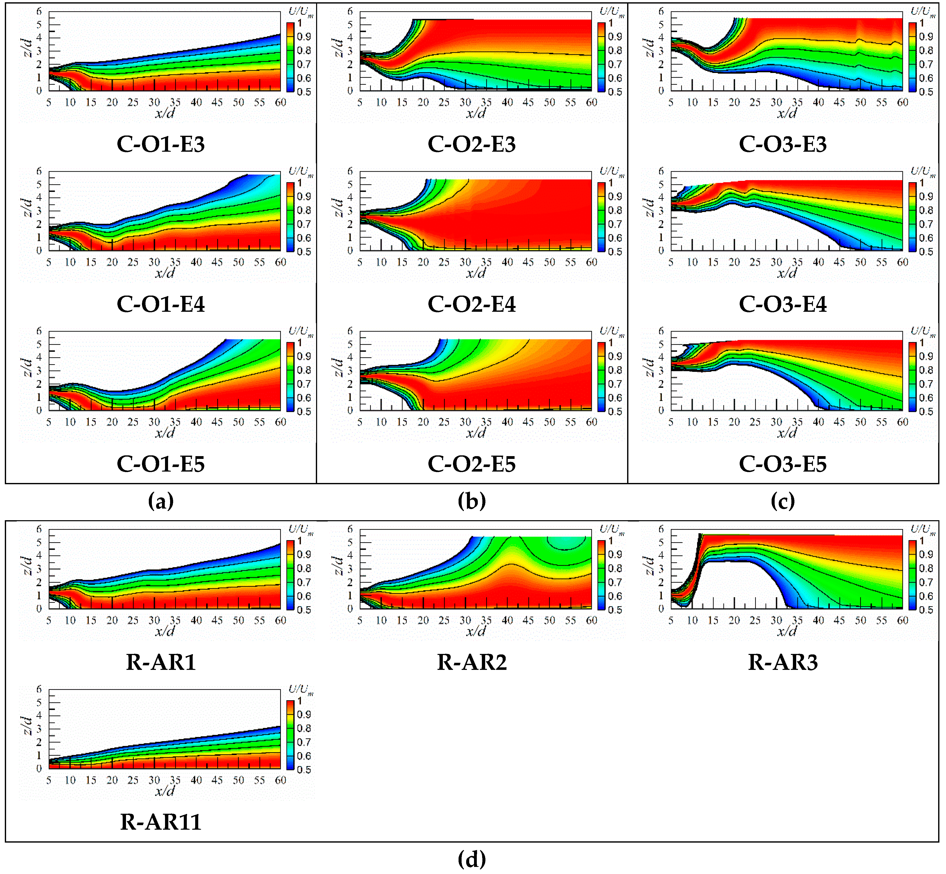
• The development of the jet within the potential core zone was observed to be dependent on the circumference of jet exits. It was noted that the length of the potential core zone decreases with the circumference of exit.
• The results showed that the development of the U_m in the transition zone could be divided into two modes. That is, (a) the decay of U_m could be estimated from power law fit with a decay rate n of 1.089–1.451 as the offset ratio is lower (OR = 1). (b) A linear fit was used to estimate the decay rates for higher offset ratio jet (OR = 2 or 3). It was observed that U_m decay is the fastest as the offset ratio (OR) is 2. Further, the results indicate that a more confining enclosure produces a more rapid jet decay than a less confining condition.
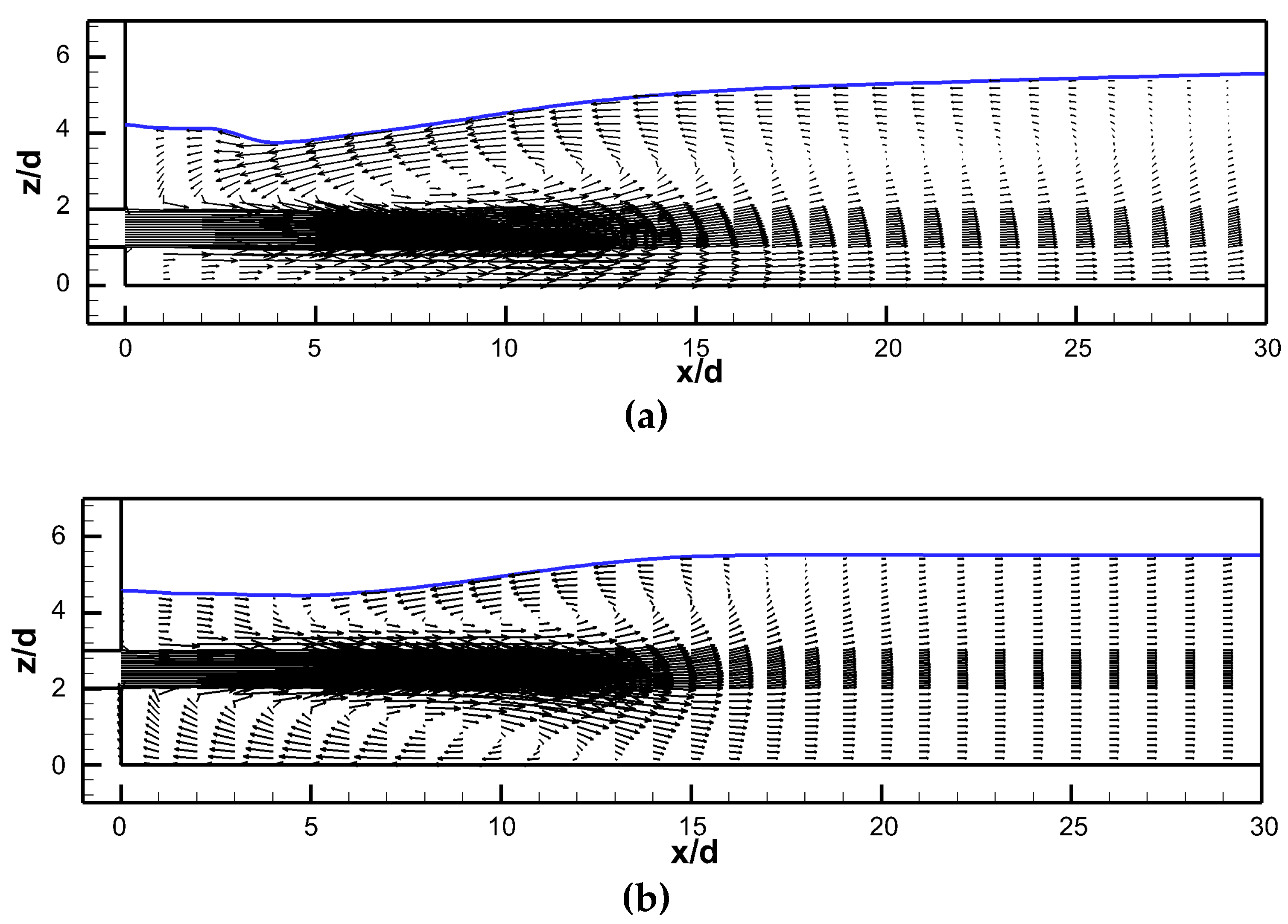
• The spread rate of the circular jet is not affected by the expansion ratios and offset ratio in the early region of jet decay. The main flow for OR = 2 was traveled straightly, and the main flow was toward the floor and the water surface as the OR = 1 and OR = 3, respectively.
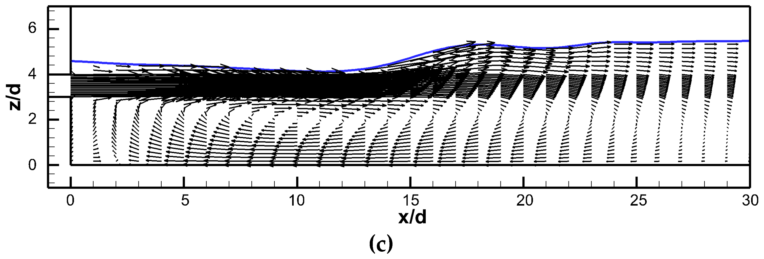
• The absence of the sudden expansion coupled with the high aspect ratio of the exit contributed to form a unique flow pattern compared with other cases.

References

1. SoaresFrazão, S. Wastewater Hydraulics; Springer: Berlin/Heidelberg, Germany, 2010; pp. 842–843. [Google Scholar]
2. Liu, M.; Rajaratnam, N.; Zhu David, Z. Mean Flow and Turbulence Structure in Vertical Slot Fishways. J. Hydraul. Eng. 2006, 132, 765–777. [Google Scholar] [CrossRef]
3. Chen, J.-G.; Zhang, J.-M.; Xu, W.-L.; Li, S.; He, X.-L. Particle image velocimetry measurements of vortex structures in stilling basin of multi-horizontal submerged jets. J. Hydrodyn. 2013, 25, 556–563. [Google Scholar] [CrossRef]
4. Dey, S.; Ravi Kishore, G.; Castro-Orgaz, O.; Ali, S.Z. Hydrodynamics of submerged turbulent plane offset jets. Phys. Fluids 2017, 29, 065112. [Google Scholar] [CrossRef]
5. Bhuiyan, F.; Habibzadeh, A.; Rajaratnam, N.; Zhu David, Z. Reattached Turbulent Submerged Offset Jets on Rough Beds with Shallow Tailwater. J. Hydraul. Eng. 2011, 137, 1636–1648. [Google Scholar] [CrossRef]
6. Durand, Z.M.J.; Clark, S.P.; Tachie, M.F.; Malenchak, J.; Muluye, G. Experimental Study of Reynolds Number Effects on Three-Dimensional Offset Jets. In Proceedings of the 12th International Conference on Nanochannels, Microchannels, and Minichannels, Chicago, IL, USA, 3–7 August 2014. [Google Scholar] [CrossRef]
7. Nyantekyi-Kwakye, B.; Tachie, M.F.; Clark, S.P.; Malenchak, J.; Muluye, G.Y. Experimental study of the flow structures of 3D turbulent offset jets. J. Hydraul. Res. 2015, 53, 773–786. [Google Scholar] [CrossRef]
8. Agelin-Chaab, M.; Tachie, M.F. Characteristics and structure of turbulent 3D offset jets. Int. J. Heat Fluid Flow 2011, 32, 608–620. [Google Scholar] [CrossRef]
9. Li, J.-N.; Zhang, J.-M.; Peng, Y. Characterization of the mean velocity of a circular jet in a bounded basin. J. Zhejiang Univ. Sci. A 2017, 18, 807–818. [Google Scholar] [CrossRef]
10. Kumar Rathore, S.; Kumar Das, M. Effect of Freestream Motion on Heat Transfer Characteristics of Turbulent Offset Jet. J. Therm. Sci. Eng. Appl. 2015, 8, 011021. [Google Scholar] [CrossRef]
11. Camino, G.A.; Zhu, D.Z.; Rajaratnam, N. Jet diffusion inside a confined chamber. J. Hydraul. Res. 2012, 50, 121–128. [Google Scholar] [CrossRef]
12. Zhang, Z.; Guo, Y.; Zeng, J.; Zheng, J.; Wu, X. Numerical Simulation of Vertical Buoyant Wall Jet Discharged into a Linearly Stratified Environment. J. Hydraul. Eng. 2018, 144, 06018009. [Google Scholar] [CrossRef] [Green Version]
13. Assoudi, A.; Habli, S.; Mahjoub Saïd, N.; Bournot, H.; Le Palec, G. Three-dimensional study of turbulent flow characteristics of an offset plane jet with variable density. Heat Mass Transf. 2016, 52, 2327–2343. [Google Scholar] [CrossRef]
14. Mondal, T.; Guha, A.; Das, M.K. Computational study of periodically unsteady interaction between a wall jet and an offset jet for various velocity ratios. Comput. Fluids 2015, 123, 146–161. [Google Scholar] [CrossRef]
15. Vishnuvardhanarao, E.; Das, M.K. Computation of Mean Flow and Thermal Characteristics of Incompressible Turbulent Offset Jet Flows. Numer. Heat Transf. A 2007, 53, 843–869. [Google Scholar] [CrossRef]
16. Gu, R. Modeling Two-Dimensional Turbulent Offset Jets. J. Hydraul. Eng. 1996, 122, 617–624. [Google Scholar] [CrossRef]
17. Hnaien, N.; Marzouk, S.; Ben Aissia, H.; Jay, J. CFD investigation on the offset ratio effect on thermal characteristics of a combined wall and offset jets flow. Heat Mass Transf. 2017, 53, 2531–2549. [Google Scholar] [CrossRef]
18. Abraham, J.; Magi, V. Computations of Transient Jets: RNG k-e Model Versus Standard k-e Model; SAE: Warrendale, PA, USA, 1997. [Google Scholar]
19. Nasr, A.; Lai, J.C.S. A turbulent plane offset jet with small offset ratio. Exp. Fluids 1998, 24, 47–57. [Google Scholar] [CrossRef]
20. Launder, B.E.; Sharma, B.I. Application of the energy-dissipation model of turbulence to the calculation of flow near a spinning disc. Lett. Heat Mass Transf. 1974, 1, 131–137. [Google Scholar] [CrossRef]
21. Bai, Z.; Wang, Y.; Zhang, J. Pressure distributions of stepped spillways with different horizontal face angles. In Proceedings of the Institution of Civil Engineers-Water Management; Thomas Telford Ltd.: London, UK; pp. 1–12.
22. Li, S.; Zhang, J. Numerical Investigation on the Hydraulic Properties of the Skimming Flow over Pooled Stepped Spillway. Water 2018, 10, 1478. [Google Scholar] [CrossRef]
23. Hirt, C.W.; Nichols, B.D. Volume of Fluid (VOF) Method for the Dynamics of Free Boundaries. J. Comput. Phys. 1981, 39, 201–225. [Google Scholar] [CrossRef]
24. Peng, Y.; Mao, Y.F.; Wang, B.; Xie, B. Study on C–S and P–R EOS in pseudo-potential lattice Boltzmann model for two-phase flows. Int. J. Mod. Phys. C 2017, 28, 1750120. [Google Scholar] [CrossRef]
25. Peng, Y.; Wang, B.; Mao, Y. Study on Force Schemes in Pseudopotential Lattice Boltzmann Model for Two-Phase Flows. J. Math. Probl. Eng. 2018, 2018, 9. [Google Scholar] [CrossRef]
26. Peng, Y.; Zhang, J.; Meng, J. Second-order force scheme for lattice Boltzmann model of shallow water flows. J. Hydraul. Res. 2017, 55, 592–597. [Google Scholar] [CrossRef]
27. Peng, Y.; Zhang, J.M.; Zhou, J.G. Lattice Boltzmann Model Using Two Relaxation Times for Shallow-Water Equations. J. Hydraul. Eng. 2016, 142, 06015017. [Google Scholar] [CrossRef]
28. Peng, Y.; Zhou, J.G.; Burrows, R. Modeling Free-Surface Flow in Rectangular Shallow Basins by Using Lattice Boltzmann Method. J. Hydraul. Eng. 2011, 137, 1680–1685. [Google Scholar] [CrossRef]
29. Peng, Y.; Zhou, J.G.; Burrows, R. Modelling solute transport in shallow water with the lattice Boltzmann method. Comput. Fluids 2011, 50, 181–188. [Google Scholar] [CrossRef]
30. Van Doormaal, J.P.; Raithby, G.D. Enhancements of the Simple Method for Predicting Incompressible Fluid Flows. Numer. Heat Transf. 1984, 7, 147–163. [Google Scholar] [CrossRef]
31. Celik, I.; Ghia, U.; Roache, P.; Freitas, C.J. Procedure for estimation and reporting of uncertainty due to discretization in CFD applications. J. Fluids Eng. 2008, 130, 078001. [Google Scholar] [CrossRef]
32. Nyantekyi-Kwakye, B.; Clark, S.P.; Tachie, M.F.; Malenchak, J.; Muluye, G. Flow characteristics within the recirculation region of three-dimensional turbulent offset jet. J. Hydraul. Res. 2015, 53, 230–242. [Google Scholar] [CrossRef]
33. Li, X.; Wang, Y.; Zhang, J. Numerical Simulation of an Offset Jet in Bounded Pool with Deflection Wall. Math. Probl. Eng. 2017, 2017, 11. [Google Scholar] [CrossRef]
34. Nyantekyi-Kwakye, B.; Tachie, M.F.; Clark, S.P.; Malenchak, J.; Muluye, G.Y. Acoustic Doppler velocimeter measurements of a submerged three-dimensional offset jet flow over rough surfaces. J. Hydraul. Res. 2017, 55, 40–49. [Google Scholar] [CrossRef]
35. Padmanabham, G.; Lakshmana Gowda, B.H. Mean and Turbulence Characteristics of a Class of Three-Dimensional Wall Jets—Part 1: Mean Flow Characteristics. J. Fluids Eng. 1991, 113, 620–628. [Google Scholar] [CrossRef]
36. Rajaratnam, N. Turbulents Jets; Elsevier: New York, NY, USA, 1976. [Google Scholar]
37. Ohtsu, I.; Yasuda, Y.; Ishikawa, M. Submerged Hydraulic Jumps below Abrupt Expansions. J. Hydraul. Eng. 1999, 125, 492–499. [Google Scholar] [CrossRef]
Figure 1. the sketch of the submerged offset jet in a chamber. Flow divided by a relationship with bottom floor: ① recirculation region, ② impingement region, and ③ wall jet region.
Water 11 00059 g001
Figure 2. Layout of the calculation (C-O3-E5).
Water 11 00059 g002
Figure 3. Sketch of jet exits.
Water 11 00059 g003
Figure 4. (a)Velocity profiles on jet exit axis with three grid sizes; (b) Results from grid 2, with discretization error bars computed using GCI.
Water 11 00059 g004
Figure 5. Experiment model.
Water 11 00059 g005
Figure 6. Model validation: (a) Heights of the water surface in streamwise direction; (b) Velocity distribution in streamwise direction (central line of exit); (c) Velocity distribution in lateral direction; (d) Velocity distribution in floor-normal direction.
Water 11 00059 g006aWater 11 00059 g006b
Figure 7. (a) Um decay for circular offset jets; (b) the relationship of LPC, ER, and OR for circular offset jets; (c) Um decay for rectangular offset jets (AR ≤ 3); (d) the relationship of LPC and Lexit.
Water 11 00059 g007
Figure 8. (a) power law fit to Um for circular offset jets as OR = 1; (b) linear fit to Um for circular offset jets as OR = 2; (c) linear fit to Um for circular offset jets as OR = 3; (d) power law or linear fit to Um for rectangular offset jets.
Water 11 00059 g008
Figure 9. Velocity vectors of offset jet with different offset ratio: (a) OR = 1 (C-O1-E4); (b) OR = 2 (C-O2-E4); (c) OR = 3 (C-O3-E4).
Water 11 00059 g009aWater 11 00059 g009b
Figure 10. Streamwise mean velocity distribution in symmetry (x–z) plane: (a) circular offset jets (ER = 4); (b) rectangular offset jets.
Water 11 00059 g010aWater 11 00059 g010b
Figure 11. Contour of U/Um in symmetry (x–z) plane: (a) circular offset jets (ER = 3); (b) circular offset jets (ER = 4); (c) circular offset jets (ER = 4.8); (d) rectangular offset jets.
Water 11 00059 g011
Figure 12. Profiles of U/Um in (x–y) plane of circular jet.
Water 11 00059 g012