Method for the Calculation of the Underwater Effective Wake Field for Propeller Optimization

Abstract

A quasi-steady prediction model of propeller hydrodynamic performance was established here using the surface panel method to determine the effective wake field of a propeller. The apparent wake field was accurately determined in advance by CFD (Computational Fluid Dynamics). The average of the induced velocity near the front of the propeller was determined by coupling the steady calculation and the unsteady forecast to render the induced velocity field more consistent with the actual situation when the propeller works in a non-uniform flow field. By superimposing the induced velocity near the front of the propeller with the apparent wake field, the effective wake field was able to be determined. Then the induced velocity field was calculated again to determine the new effective wake. An iterative calculation method was used until the hydrodynamic performance converged. The case described here shows that the effective wake obtained by this method can better predict the hydrodynamic performance of the propeller, and it can provide a basis for the design and optimization of the propeller. It was found that the results of the prediction were consistent with the experimental values.

1. Introduction

With the development of high-speed ships, high-power hosts have been in widespread use. A series of new problems have emerged in ship performance, such as tail vibration, structural defects, noise and erosion. The basic reason for this is that local variable cavitation and a strong pulse exciting force are produced when the propeller works in a non-uniform wake and the propeller’s load increases. To improve this situation, accurate testing and methods of forecasting the wake are needed.

A ship’s wake is the non-dimensional velocity component at the disk of the propeller. Using different methods of measurement, it can be classified as a nominal wake or an effective wake, which differ in whether the work of the propeller is considered. When working in the stern, the propeller produces a suction effect that changes the stern flow, thickness of the boundary layer, waveforms, and other factors. It is reasonable to calculate propeller performance using the effective wake. The first studies of the effective wake were published relatively recently, starting in the 1970s. Nelson of the San Diego Naval Undersea Center, Huang Chongzhi et al. of DTNSRDC (David Taylor Naval Ship R&D Center), and Nagamatsu, and Tokunaga of the Mitsubishi Heavy Industries Nagasaki Test Tank in Japan began theoretical studies of the effective wake [1] Since then, teams led by Todd, Kinnas, Chios, Apurva, and Hua have carried out a great deal of experimental and theoretical research work and have made advances in effective wake distribution [2,3,4,5,6,7,8]. Huang and Wang (1976) succeeded in using a laser Doppler velocimeter to measure the velocity distribution quite close to the propeller disk. Their results provided information on the mutual influence between the propeller and the stern boundary layer. After the measurement, they developed a theoretical method for determining the effective wake [9,10]. The predicted axial velocity results produced by this method were closely consistent with the data measured near the front of the propeller. Domestic scholars also have carried out some studies of the effective wake, on the basis of the method of prediction in single-screw ships of ITTC (International Towing Tank Conference) 1978. Wu (1994) modified the formula used to calculate the fraction of the wake of a ship with real dimensions. This made up for the low power and rotation speed forecast using this method [11]. In 1982, Wang et al. from the Dalian Institute of Technology brought forward a theoretical calculation method for model ship wake analysis according to the test results for a model wake. They made further developments in 1987, and provided a method of analyzing the model ship wake correlation to calculate the potential wake on the propeller disk after using the three-dimensional potential flow [12,13]. In 1983, Qian of the China Shipbuilding and Marine Engineering Design and Research Institute measured apparent velocity by using the ship model to drive the propeller and calculate the effective wake according to expanded lifting line theory [14].

From the analysis provided above, the current state of the research on effective wake has been limited to the level of experimentation and lifting line theory. The surface panel method, a theory for the prediction of the hydrodynamic performance and the disturbance field of the propeller, has been proven reliable. In this paper, a quasi-steady hydrodynamic performance prediction model is established using the surface panel method to determine the induced velocity near the front of the propeller working in the non-uniform wake field of the stern. Then the effective wake can be obtained by superimposing the included velocity with the obtained apparent wake. The KCS (KRISO Container Ship) was used as an example to verify this method. Obtaining precise underwater effective wake field can better predict the hydrodynamic performance of the propeller, and it can provide a basis for the design and optimization of the propeller.

2. Numerical Calculation Method

2.1. Basic Formula

Considering that a propeller turns with angular velocity ω in the irrotational, inviscid, and incompressible fluid, the inflow is non-uniform and the speed is ${\mathit{V}}_a(x,y,z,t)$.

As shown in Figure 1, O-XYZ is the space fixed coordinate system, O-xyz is the rectangular coordinate system fixed on the blades, O-xrθ is the cylindrical coordinate system fixed on the blades, θ is the rotation angle from the start of the Z axis along the direction of propeller rotation. The relative inflow velocity of the propeller is as follows:

$${\mathit{V}}_0(x,y,z,t)={\mathit{V}}_a(x,y,z,t)+\omega r$$

(1)

The propeller perturbation velocity field can be described by the disturbance velocity potential φ(t), and φ(t) meets the Laplace equation, which is as follows:

$${\nabla }^2\phi (t)=0$$

(2)

According to the Green theorem, the velocity potential of any point can be expressed as follows:

$$4\pi E\phi (P,t)={\displaystyle \underset{S}{\iint }[\phi (Q,t)\frac{\partial }{\partial n_Q}(\frac{1}{R_{PQ}})}-\frac{\partial \phi (Q,t)}{\partial n_Q}\frac{1}{R_{PQ}}]dS$$

(3)

where:

$$E=\{\begin{array}{c}0PisinsideofS\\ 1/2PisontheS\\ 1PisoutofS\end{array}$$

Similar to the steady problems, the disturbance velocity potential φ(t) should also satisfy the following conditions:

$$\nabla \phi (t)\to 0,S_{\infty }\to \infty$$

(4)

$$\frac{\partial \phi (t)}{\partial n_Q}=-{\mathit{V}}_0(x,y,z,t)\cdot {\mathit{n}}_{Q}P\mathrm{is}\mathrm{on}\mathrm{the}{S}_B$$

(5)

$$\begin{array}{r}{p}^{+}-p^{-}=0\\ {(\frac{\partial \phi (t)}{\partial n_{Q_1}})}^{+}-{(\frac{\partial \phi (t)}{\partial n_{Q_1}})}^{-}=0\end{array}P\mathrm{is}\mathrm{on}\mathrm{the}{S}_W$$

(6)

where $S_{\infty }$, $S_B$, and $S_W$ represent the outside interface, the surface of propeller, and the surface of the tail vortex, respectively. Considering the three conditions above, on the boundary surface the integral Equation (3) can be written as follows:

$$\begin{array}{ll}2\pi \phi (P,t)& ={\displaystyle \underset{S_B}{\iint }\phi (Q,t)\frac{\partial }{\partial n_Q}(\frac{1}{R_{PQ}})dS}+{\displaystyle \underset{S_W}{\iint }\Delta \phi (Q_1,t)}\frac{\partial }{\partial n_Q{}_1}\frac{1}{R_{P{Q}_1}}dS\\ & +{\displaystyle \underset{S_B}{\iint }({\mathit{V}}_0(t)\cdot {\mathit{n}}_Q)}(\frac{1}{R_{PQ}})dSon{S}_B\end{array}$$

(7)

where $\Delta \phi (Q_1,t)$ is the potential jump across the wake surface, which can be expressed as follows:

$$\Delta \phi (Q_1,t)=\phi {(Q_1,t)}^{+}-\phi {(Q_1,t)}^{-}on{S}_w$$

(8)

Equation (9) is a function of time and location, at any time t, the value most near the trailing edge can be determined by the following pressure Kutta condition:

$${(\Delta p)}_{TE}(t)=p_{TE}^{+}(t)-p_{TE}^{-}(t)=0$$

(9)

Therefore, at any moment, the numerical solution of Equation (8) can be made out. It is the disturbance velocity potential on the surface of the propeller. Taking the derivative of this velocity potential, the disturbance velocity on the surface of the propeller $\mathit{V}(x,y,z,t)$ is obtained. The total velocity on the surface of the propeller is the resultant velocity of the disturbance velocity and the inflow velocity, which is as follows:

$${\mathit{V}}_t(x,y,z,t)={\mathit{V}}_0(x,y,z,t)+\mathit{V}(x,y,z,t)$$

(10)

According to the Bernoulli theorem, the pressure on the surface of the propeller can be expressed as follows:

$$p(t)=p_0+\frac{1}{2}\rho [|{\mathit{V}}_0(t){|}^2-|{\mathit{V}}_t(t){|}^2]-\rho \frac{\partial \phi (t)}{\partial t}$$

(11)

At any time, the way to solve the basic Equation (8) is similar to the steady problem. However, as a function of time and location, the unknown variables $\Delta \phi (Q_1,t)$ in the basic equation cannot be determined by the Kutta condition, and only the value nearest the blade trailing edge can be calculated. Thus, time domain calculation methods must be developed to solve the unsteady problem. The method provided by [15] is used here.

Eventually, the hydrodynamic performance of propeller is expressed as follows:

$$K_T=\frac{T}{\rho n^2{D}^4};K_Q=\frac{Q_{}}{\rho n^2{D}^5};{\eta }_{}=\frac{K_T}{K_Q}\frac{J}{2\pi }$$

(12)

where K_T and K_Q are propeller thrust coefficient and torque coefficient, η is the efficiency of the propeller, T and Q represent the propeller’ thrust and torque, J is the advance coefficient, ρ is the fluid density, D is the propeller’s diameter, and n is propeller’s rotational speed.

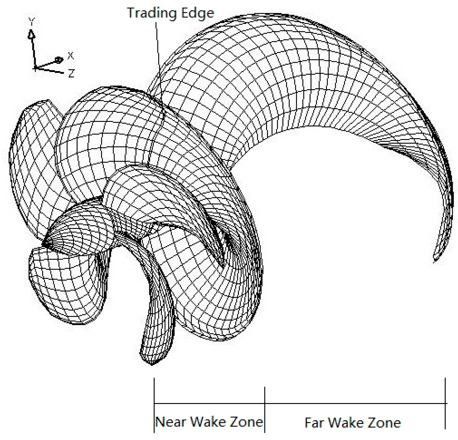
2.2. Numerical Calculation of the Unsteady Propeller-Induced Velocity Field

For the study of the propeller-induced velocity field, the lifting line theory and the lifting surface theory are usually used. Because the lifting line vortex model is so simple that the propeller hydrodynamic performance and the calculation of the induced velocity field cannot be predicted accurately enough, only the circumferential average of the induced velocity after the propeller can be calculated [16]. Even though the lifting surface theory can accurately forecast the hydrodynamic performance of the propeller for the calculation of the induced velocity field, there is still a large error, especially near the propeller. However, the calculation model of the surface panel method can simulate the propeller and its working performance more accurately. Thus, for the velocity distribution near the propeller, the calculation of the velocity distribution consistent with the actual calculation results can be obtained.

The induced velocity field of the propeller in unsteady conditions remains similar to the steady condition. For some time, t, taking the gradient to the both sides of Equation (8) can produce the induced velocity expression of field point P (due to the fact that the calculation points are in the flow field, so E takes 1):

$$\begin{gathered} 4\pi V(P,t)={\displaystyle \underset{S_B}{\iint }\phi (Q,t){\nabla }_P\frac{\partial }{\partial n_Q}(\frac{1}{R_{PQ}})dS}+{\displaystyle \underset{S_W}{\iint }\Delta \phi (Q_1,t){\nabla }_P\frac{\partial }{\partial n_{Q1}}(\frac{1}{R_{P{Q}_1}})dS} \\ +{\displaystyle \underset{S_B}{\iint }(V_0(t)\cdot n_Q){\nabla }_P(\frac{1}{R_{PQ}}})dS \end{gathered}$$

(13)

For the propeller rotating with speed ω in the non-uniform flow, the calculation can be started at any time. The time step takes ∆t, and the corresponding rotation angle step length is $\Delta \theta =\omega \Delta t$. Suppose that the initial time is $t_0=0$ and the first blade is in the $\theta =0$ at this point. Then during step k_t, the time is $k_t\Delta t$, and the first blade’s angle position is $k_t\Delta \theta$. The blades are numbered along the direction of ${\theta }_1$, and the number k blade is in the position of $k_t\Delta \theta -2\pi (k-1)/Z$.

Taking the same method as with the steady problem, the surfaces of the propeller and the trailing vortex surface are divided into small units, and the hyperboloid elements are used to replace each unit approximately. The panel number on one blade and one Z of the propeller hub is $N_P=2N_C{N}_R+N_H$, and the panel number of one tail vortex surface is $N_R{L}_W$. L_W is the panel number along the trail vortex line. It should be infinite, but the number is usually very large.

The disturbance velocity potential φ(t), velocity potential jump ∆φ(t) and $[{\mathit{V}}_0(t)\cdot \mathit{n}]$ are believed to be distributed evenly on each panel. Taking the shape heart of the panel as the control point, at the step k_t, the induced velocity Equation (15) at the flow field point P_i can be described as follows:

$$\begin{gathered} \mathit{V}(P_i,t)={\displaystyle \sum _{k=1}^Z{\displaystyle \sum _{j=1}^N{\phi }_j^k(k_t\Delta t){\nabla }_P{C}_{ij}^k}}+{\displaystyle \sum _{k=1}^Z{\displaystyle \sum _{m=1}^{N_R}{\displaystyle \sum _{l=1}^{L_W}\Delta {\phi }_{ml}^k(k_t\Delta t){\nabla }_P{W}_{iml}^k}}} \\ +{\displaystyle \sum _{k=1}^Z{\displaystyle \sum _{j=1}^{N_P}(V_{ij}^k(k_t\Delta t)\cdot n_j^k){\nabla }_P{B}_{ij}^k}} \end{gathered}$$

(14)

where ${\nabla }_P{C}_{ij}^k$, ${\nabla }_P{C}_{ij}^k$ and ${\nabla }_P{B}_{ij}^k$ are influence coefficients defined by the following formulas:

$$\{\begin{array}{l}{\nabla }_P{C}_{ij}^k=\frac{1}{4\pi }{\displaystyle \underset{S_j^k}{\iint }{\nabla }_P\frac{\partial }{\partial n_j^k}(\frac{1}{R_{ij}^k})d{S}_j^k}\\ {\nabla }_P{W}_{iml}^k=\frac{1}{4\pi }{\displaystyle \underset{S_{ml}^k}{\iint }{\nabla }_P\frac{\partial }{\partial n_{ml}^k}(\frac{1}{R_{iml}^k})d{S}_{ml}^k}\\ {\nabla }_P{B}_{ij}^k=\frac{-1}{4\pi }{\displaystyle \underset{S_j^k}{\iint }{\nabla }_P\frac{\partial }{\partial n_j^k}(\frac{1}{R_{ij}^k})d{S}_j^k}\end{array}$$

(15)

where $S_j^k$ and $S_{ml}^k$ are the panel area of the number k blade and the trailing vortex sheet, $R_{ij}^k$ and $R_{iml}^k$ are the distance from $P_i$ to the integral points on $S_j^k$ and $S_{ml}^k$, respectively. ${\nabla }_P{C}_{ij}^k$, ${\nabla }_P{W}_{iml}^k$ and ${\nabla }_P{B}_{ij}^k$ can be determined through the method supplied by Morino et al. [17].

During the calculation process, first, the strength of the source-sink and dipole distributed on the surface of the propeller and the trailing vortex sheet are worked out under the unsteady conditions. Then the velocity induced at any spatial point is calculated using Equation (13). The induced velocity is added near the front of the propeller to the apparent wake to produce the effective wake. Usually, the wake that can be obtained directly is the apparent wake.

During the numerical calculation, the second iteration in Equation (13) will produce an unreasonable result when the calculation point in the flow field is very close to the trailing vortex sheet. In this situation, the dipole on the trailing vortex sheet panel close to the calculation point should be converted to vortex circulation using the equivalence relationship between the normal dipole and vortex ring. Then the induced velocity on this panel can be calculated using the method put forward by Kervin, who considered the influence of blade thickness and calculated the propeller performance using the discretization method [18,19,20].

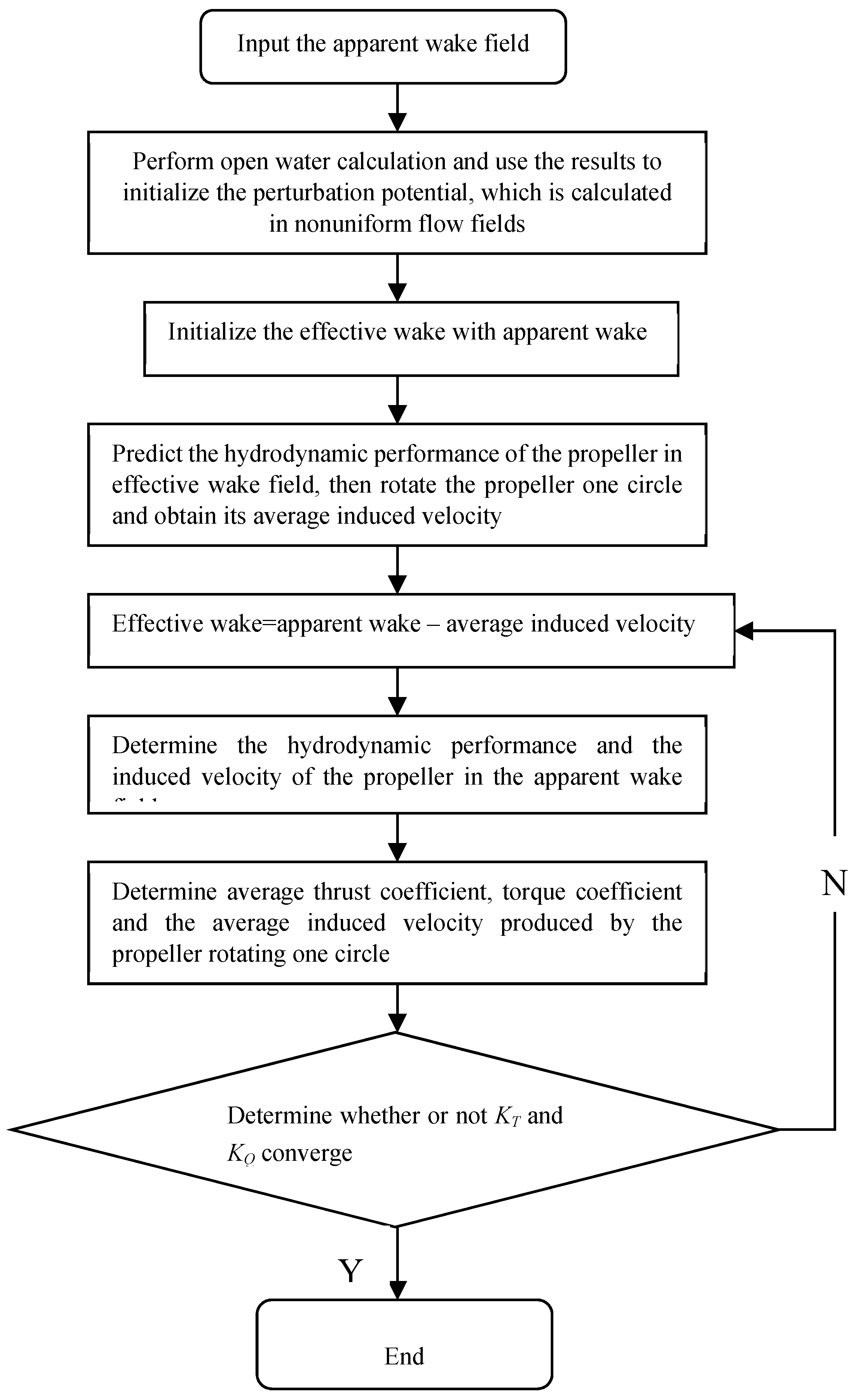
2.3. Iterative Calculation Process

First, forecast the steady performance of the propeller in open water and convert the results of the steady calculation to the initial value of the unsteady performance forecast. In the process of unsteady calculation, use the obtained apparent wake to initialize the effective wake before the first iteration and calculate the average hydrodynamic performance of the propeller for one revolution and the average induced velocity near the front of the propeller. The first approximate effective wake can be determined by adding the induced velocity to the apparent wake. Then, the hydrodynamic performance and induced velocity near the front of propeller in each time step are calculated in this effective wake. After that, determine whether the hydrodynamic performance converges. If so, the iteration is ended. Otherwise, the new induced velocity is added to the apparent wake, so the new effective wake can be gained. This iterative process is then repeated until the obtained thrust coefficient K_T and the torque coefficient K_Q of the propeller converge. The final wake gained is the effective wake. The iterative process is shown in Figure 2.

3. Instance Verification

3.1. Model Introduction

The KCS ship was chosen as the authentication object to confirm the effective wake field acquisition method proposed in this paper, and comparisons were drawn between the experimental results. The KCS ship is a 3600 TEU container vessel designed and built by KRISO (Korea Research Institute of Ships & Ocean Engineering) of South Korea [21]. It was chosen as a benchmark model for use in the international shipping computation fluid dynamics workshop, and there were a considerable number of detailed test data and other numerical results available. This ship has a tail flow field with obvious features. This provides the user with a convenient way of checking the calculation results.

Table 1. Main parameters of the KCS model.

Length between Perpendiculars (m)	Molded Breadth (m)	Draft (m)	Wetted Surface (m)	Block Coefficient	Advance Coefficient
7.2786	1.0190	0.3418	9.438	0.65	0.925

provides the main parameters of the ship model. The speed of the real ship is 24 kn, and the scale ratio is 31.599.

The model propeller is KP505, its main parameters are shown in

Table 2. Main parameters of the KP505 propeller model.

Number of Blades	Profile Type	Scale Ratio	Propeller Diameter (m)	Boss Ratio
5	NACA66 + a = 0.8	31.599	0.25	0.18

. The propeller installation position is in the position of x/L = 0.4825, namely after perpendicular 0.0175 L (127.3 mm) upstream, where x is the coordinate along the direction of the hull length, and L is the ship model length.

Although using a tank experiment is accurate and credible for determining the apparent wake field of the ship, it is highly expensive. This paper presents a method based on the CFD technology, which can be used to determine the apparent wake distribution in the tight front of the propeller precisely with the advance coefficient of the model 0.925.

Table 3. KCS resistance calculation results with propeller.

	Calculated Value	Experimental Value	Error
Hull resistance (N)	91.8	90	2%
Propeller thrust (N)	58.5	59.9	2.34%
Propeller torque (N.m)	2.47	2.53	2.47%

provides the KCS resistance calculation results with the propeller. The speed of the ship model is 2.196 m/s and the rotating speed of the propeller is 9.5 rps. A moving reference frame (MRF) model was used in the calculation. When solving the calculation, the SIMPLEC (Semi-ImplicitMethod for Pressure Linked Equations-Consistent) algorithm was selected for the pressure–velocity coupling, and PRESTO was selected in pressure discrete format. Second order upwind was selected in momentum, turbulent kinetic energy, turbulent move dissipation rate discrete format, and the default values were adopted in under-relaxation factors.

It was determined that the numerical computation was highly precise by comparing with the experimental value, thus it was determined that the obtained apparent wake was reasonably accurate. In Figure 3, the distribution value is the ratio of wake and ship speed; the figure shows that the wake field in front of the propeller was no longer bilaterally symmetrical because of the mutual interference between the hull and the propeller, and that it has a visible difference from the open-water propeller wake field and no longer presents a regular shape.

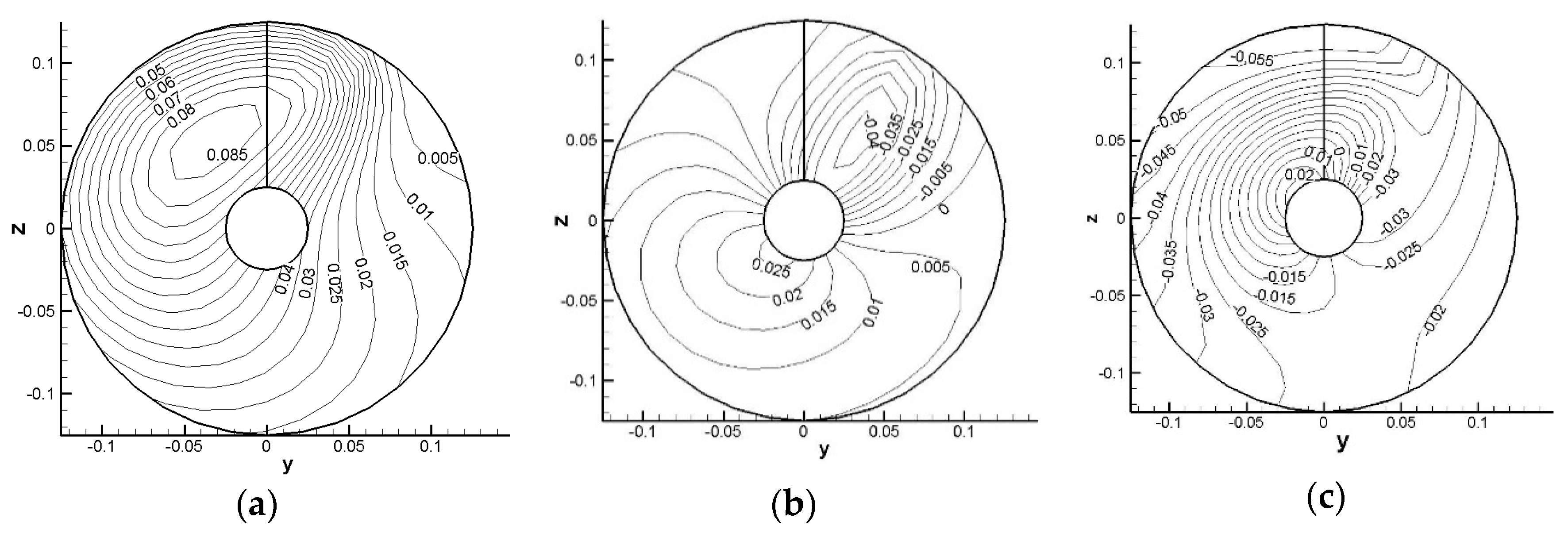
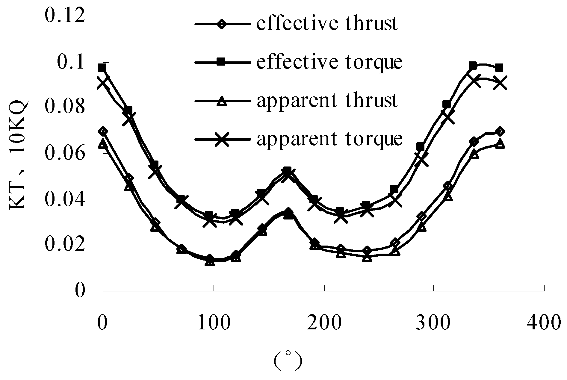
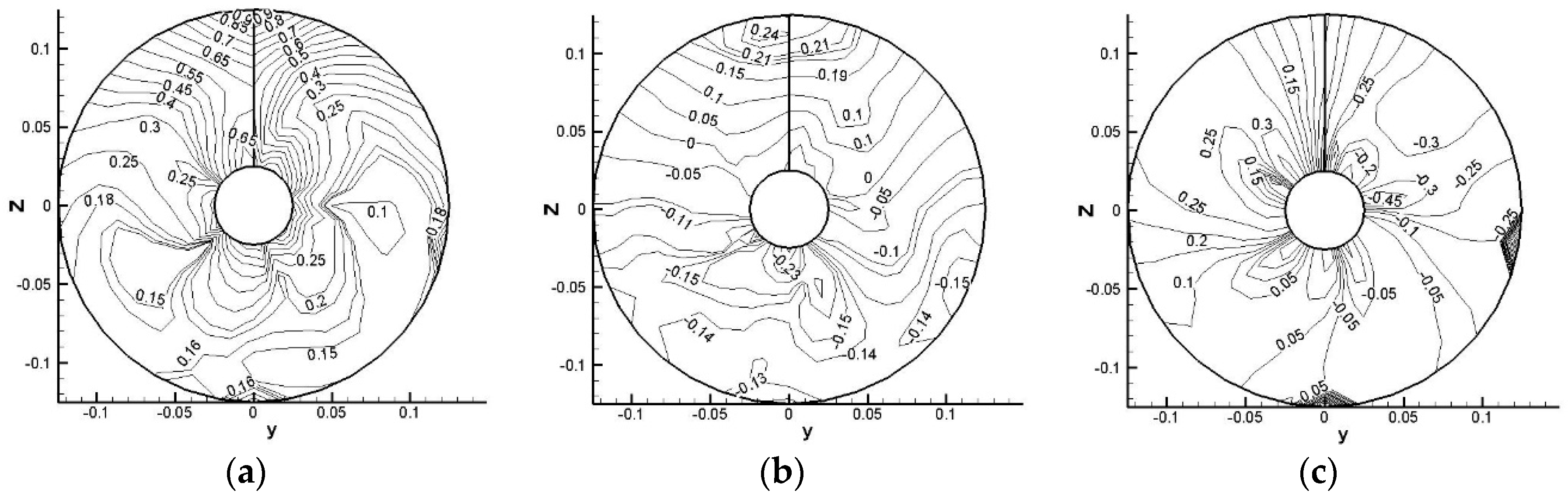
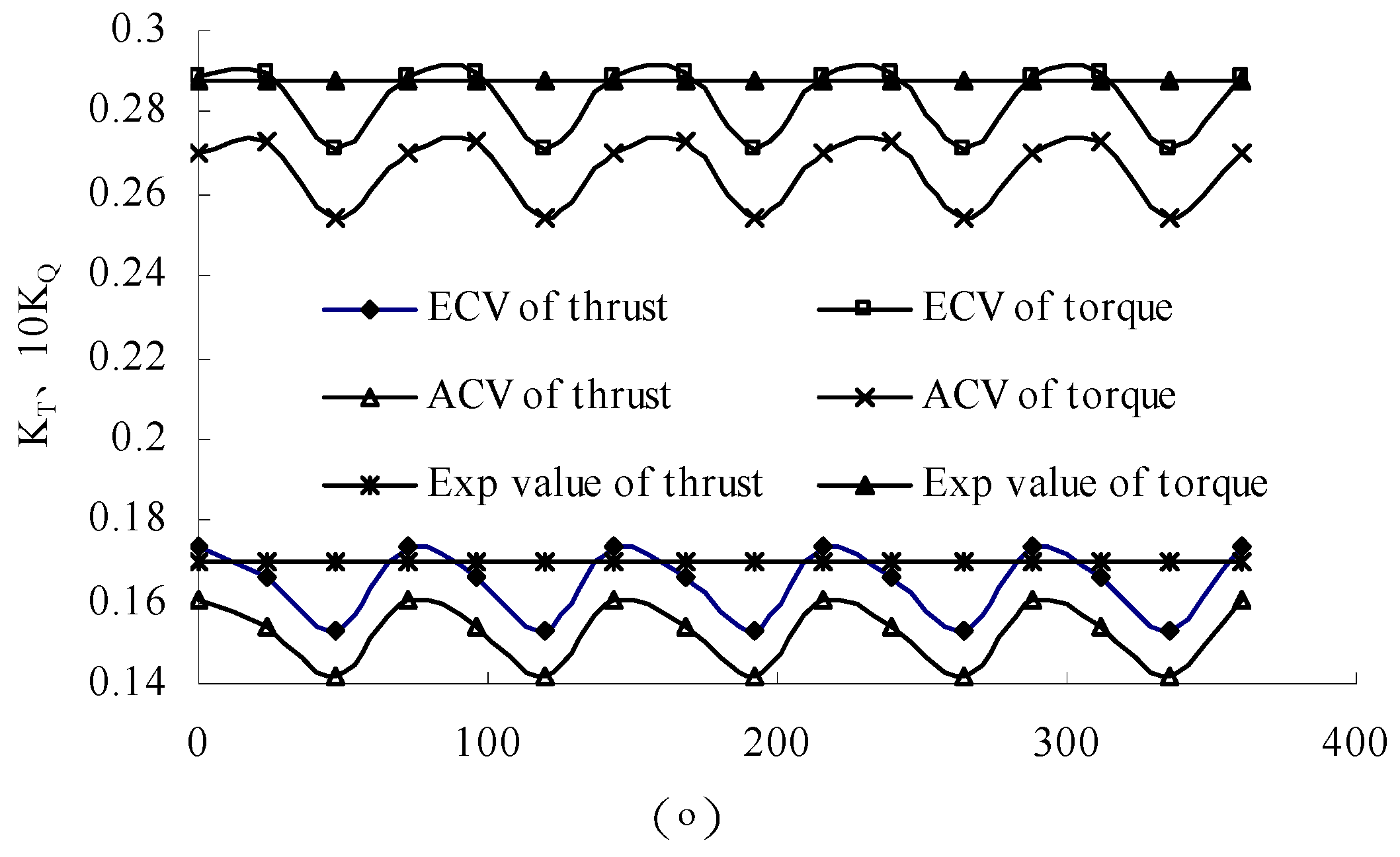
3.2. Effective Wake Analysis

During the calculation process, the cosine spacing was employed in the chordwise direction and spanwise direction of the propeller blade. In order to make the calculation results closer to the experimental value, this paper adopted the nonlinear trailing vortex contraction model [22]. The trailing vortex model was divided into two areas, the near wake zone and the far wake zone. The near wake zone was from the blade trailing edge to downstream of one diameter where the trailing vortex was already total shrinkage. It had a smooth transition in the middle radius, and the pitch angle of the trailing vortex surface changed in the radius and downstream direction. The pitch angle and the radius in the far wake zone remained constant in the radius and downstream direction. The division of the propeller and trailing vortex surface elements is shown in Figure 4.

The method proposed in this paper can be used to determine the effective wake in front of the blade and predict the hydrodynamic performance of the KP505 propeller under the effective wake. Through the quasi-steady calculating iteration, the induced velocity (m/s) in the tight front of the propeller with the hydrodynamic performance converging is shown in Figure 5. Overlaying the apparent wake in Figure 3 and the induced velocity in Figure 5 in the axial, circumferential, and radial direction, then the final effective wake can be determined.

Figure 6 shows the changing trend of the thrust and torque of the key propeller blade in the final converging condition, which can be used to compare the forecast results collected using the effective wake with those collected using the apparent wake. As shown in the figure, the results of the calculations produced using the effective wake and apparent wake remained consistent, and the calculated effective wake was larger. When the key blade rotated to the left, the calculated results of the effective wake field were significantly larger than those of the apparent wake field. This is mainly because the propeller can make a strong disturbance in the flow field on the left side, as shown in Figure 5, so the propeller’s effective advance speed was smaller than the apparent advance speed.

Figure 7 shows the thrust and torque produced by the propeller rotating one cycle when using effective wake and apparent wake, compared with the experimental value. As the propeller rotates one cycle, the thrust and torque both present five repeated cycles. This is because the model propeller has five blades. The calculated results for thrust and torque remain consistent if the two kinds of wake are both considered and the calculated results of the effective wake are significantly larger than those of the apparent wake.

This paper carried out a mean error analysis of the calculated results, and the analysis results are shown in

Table 4. Error analysis.

	KT	10KQ
ECV	0.16554	0.2828
ACV	0.14049	0.2453
Experimental value	0.17030	0.2880
error of ECV	2.7%	1.80%
error of ACV	17.5%	15.2%

. The error produced by adopting the apparent wake was too large to be used to predict unsteady hydrodynamic performance directly. If the effective wake obtained through the method proposed in this paper is used, the results are much more similar to the experimental value.

4. Conclusions

This paper established a quasi-steady hydrodynamic performance prediction model for a propeller by using the surface panel method to forecast the induced velocity field near the front of the propeller. By overlaying the induced velocity field with the apparent wake field, which was determined beforehand using CFD technology, the effective wake field was also determined. The calculation results from the provided example show that the apparent wake field cannot be used directly for the unsteady hydrodynamic performance prediction. The effective wake obtained using the method proposed in this paper makes the prediction of the hydrodynamic performance of the propeller more consistent with the experimental value. In this way, it proves that this paper’s method is an effective means of determining the effective wake field in front of a propeller. This method is significantly more accurate than the unsteady hydrodynamic performance prediction of ship propeller motion. Propeller designers can use this method to obtain an accurate underwater effective wake field and predict the hydrodynamic performance of the propeller more accurately, which can help to optimize the design scheme of the propeller.

References

1. Zhou, L.D. Research status of effective wake distribution theoretical prediction. Sh. Mech. Intel. 1982. (In Chinese) [Google Scholar]
2. Taylar, T.E. Combined Experimental and Theoretical Determination of Effective for a Marine Propeller. Ph.D. Thesis, Massachusetts Institute of Technology, Cambridge, MA, USA, 1994. [Google Scholar]
3. Kinnas, S.A.; Pyo, S. Cavitating propeller analysis including the effects of wake alignment. J. Ship Res. 1999, 43, 38–47. [Google Scholar]
4. Choi, J.K.; Kinnas, S.A. Prediction of non-axissymmetric effective wake by a three-dimension Euler solver. J. Ship Res. 2001, 45, 13–33. [Google Scholar]
5. Choi, J.K.; Kinnas, S.A. Prediction of unsteady effective wake by a Euler solver/Vortex-lattice coupled method. J. Ship Res. 2003, 47, 131–144. [Google Scholar]
6. Chios, J. Vortex Inflow-Propeller Interaction Using an Unsteady Three-Dimensional Euler Solver. Ph.D. Thesis, Department of Civil Engineering, The University of Texas at Austin, Austin, TX, USA, 2000. [Google Scholar]
7. Apurva, G. Numerical Prediction of Flows around Podded Propulsor. Ph.D. Thesis, Department of Civil Engineering, The University of Texas at Austin, Austin, TX, USA, 2004. [Google Scholar]
8. Gu, H. Numerical Modeling of Flow around Ducted Propellers. Ph.D. Thesis, Department of Civil Engineering, The University of Texas at Austin, Austin, TX, USA, 2006. [Google Scholar]
9. Huang, T.; Wang, H. Propeller/Stern Boundary Layer Interaction on Axisymmetric Bodies: Theory and Experiment; Technical. Report. DTNSRDC 76-0113; Bethesda: Rockville, MD, USA, 1976. [Google Scholar]
10. Huang, T.; Groves, N. Effective wake: Theory and experiment. In Proceedings of the 13th Symposium on Naval Hydrodynamic, Tokyo, Japan, 6–10 October 1980. [Google Scholar]
11. Wu, J.M. Investigation of the scale effect correction of wake fraction during single paddle ship performance prediction. Ships 1994, 1, 25–30. (In Chinese) [Google Scholar]
12. Wang, Y.Y.; Zhang, Z.Y.; Lao, G.S. The conversion method of wake distribution from model to ship wake fields. J. Dali. Univ. Technol. 1982, 21, 59–68. (In Chinese) [Google Scholar]
13. Wang, Y.Y.; Dai, H.H. The correlation analysis of wake fields behind ships. Ship Eng. 1987, 3, 12–18. (In Chinese) [Google Scholar]
14. Qian, W.H. Effective wake field investigation. Ship Sci. Technol. 1987, 6, 46–47. (In Chinese) [Google Scholar]
15. Su, Y.M.; Huang, S.; Ikehata, M.; Kai, H. Numerical calculation of marine propeller hydrodynamic characteristics in unsteady flow by boundary element method. Shipbuild. China 2001, 42, 93–134. [Google Scholar]
16. Su, Y.M.; Ikehata, M.; Kai, H. Numerical analysis of the flow field around marine propellers by surface panel method. Ocean Eng. 2002, 20, 44–48. (In Chinese) [Google Scholar]
17. Morino, L.; Chen, L.T.; Suciu, E.O. Steady and oscillatory subsonic and supersonic aerodynamics around complex configurations. AIAA J. 1975, 13, 368–374. [Google Scholar]
18. Kerwin, J.E.; Leopold, R. Propeller incidence due to blade thickness. JSR 1963, 7, 1–6. [Google Scholar]
19. Kerwin, J.E. Computer techniques for propeller blades section design. In Proceedings of the Second Lips Propeller Symposium, Drunen, The Netherlands, 7–31 May 1973. [Google Scholar]
20. Kerwin, J.E.; Lee, C.S. Prediction of steady and unsteady marine propeller performance by numerical lifting surface theory. Trans. SNAME 1978, 86, 8. [Google Scholar]
21. Kim, J.; Park, I.R.; Van, S.H. RANS computations for KRISO container ship and VLCC tanker using the WAVIS code. In Proceedings of the CFD Workshop Tokyo 2005, Tokyo, Japan, 9–11 March 2005; pp. 598–603. [Google Scholar]
22. Tan, T.S. Performance Prediction and Theoretical Design Research on Propeller in Non-Uniform Flow. Ph.D. Thesis, Wuhan University of Technology, Wuhan, China, 2003; pp. 53–54. (In Chinese). [Google Scholar]
Figure 1. Propeller coordinate system.
Water 11 00165 g001
Figure 2. Flowchart of the effective wake field calculation.
Water 11 00165 g002
Figure 3. Apparent wake distribution. (a) Axial wake distribution; (b) Circumferential wake distribution; (c) Radial wake distribution.
Water 11 00165 g003
Figure 4. KP505 schematic diagram.
Water 11 00165 g004
Figure 5. Induced velocity in tight front of the propeller. (a) Axial-induced velocity; (b) Circumferential-induced velocity; (c) Radial-induced velocity.
Water 11 00165 g005
Figure 6. Thrust and torque of the key blade.
Water 11 00165 g006
Figure 7. Thrust and torque of propeller. (ECV and ACV represent effective wake calculated value and apparent wake calculated value, respectively).
Water 11 00165 g007