Article

Combined Exceedance Probability Assessment of Water Quality Indicators Based on Multivariate Joint Probability Distribution in Urban Rivers

School of Civil Engineering, Shandong University, Jinan 250061, China
*
Author to whom correspondence should be addressed.
Water 2018, 10(8), 971; https://doi.org/10.3390/w10080971
Submission received: 7 May 2018 / Revised: 6 July 2018 / Accepted: 9 July 2018 / Published: 25 July 2018
(This article belongs to the Section Water Quality and Contamination)

Abstract

:
Discharge and water quality are two important attributes of rivers, although the joint response relationship between discharge and multiple water quality indicators is not clear. In this paper, the joint probability distributions are established by copula functions to reveal the statistical characteristics and occurrence probability of different combinations of discharge and multiple water quality indicators. Based on the data of discharge, ammonia nitrogen content index (NH4+) and permanganate index (CODMn) in the Xiaoqing River in Jinan, we first tested the joint change-point with the data from 1980–2016, before we focused on analyzing the data after the change-point and established the multivariate joint probability distributions. The results show that the Gaussian copula is more suitable for describing the joint distribution of discharge and water quality, while the year of 2005 is a joint change-point of water quantity and quality. Furthermore, it is more reasonable to use the trivariate joint probability distribution as compared to the bivariate distributions to reflect the exceedance probability of water quality combination events under different discharge conditions. The research results can provide technical support for the water quality management of urban rivers.

1. Introduction

Water quantity and quality are two important attributes of rivers. In recent years, the water quality of rivers is deteriorating with the development of society and economy, with water dispatching having become one of the main technologies of water quality improvement [1,2,3,4]. However, due to the disturbance of urban rivers from human activities, the relationship between water quantity and water quality has become more complicated. The relationship between a single water quality indicator and the water quantity can hardly reflect the real situation of river pollution [5]. Thus, the methods for improvement of the river water quality should be based on a correct understanding of the joint response relationship between water quantity and multiple water quality indicators.
Many scholars have simulated and predicted the river water quality from the aspects of mechanism models and non-mechanism models. The mechanism models are based on the hydrodynamic model and water quality equations in order to simulate the diffusion and attenuation process of pollutants [6,7,8]. However, due to the wide variety of influencing factors and the cognitive limitations of the real water quality, this makes the model construction and parameter determination difficult [9,10,11]. Therefore, this indicates that the simulation effect of the nature river is better than that of the urban river, which is affected by human activities. The non-mechanism model can avoid this type of problems to some extent. Sun et al. [12] used the gray model group method and the exponent smoothing method to construct a probabilistic combination prediction framework of water quality to forecast the individual indicator of chemical oxygen demand in a complex environment. After this, some new models for water quality prediction have been proposed, which integrates different non-mechanism models, such as the neural networks model, fuzzy model, and wavelet model [13,14,15]. In addition, there are also some joint models that combine hydrodynamics and water quality simulation tests [16,17]. However, most non-mechanism models require that the variables obey the same marginal distribution or that these variables need to be transformed to the same distribution, which not only leads to the loss of the original data information, but it also does not conform to the fact that variables, such as discharge and water quality, obey different marginal distributions. Meanwhile, because less emphasis is placed on the joint distribution between the variables, non-mechanism models are more suitable to use a simulation of the discharge and individual water quality indicator when compared to a simulation of the discharge and multiple water quality indicators. Copula can construct the joint probability distribution of multiple variables [18] and it does not require each variable to follow the same marginal distribution. Thus, it can effectively preserve the nature of the original data. Copula has the advantages of great adaptability and flexibility, so it has been widely used in the field of hydrology, especially in determining flood risks [19,20,21,22] and drought characteristics [23,24,25,26,27,28]. However, copula has been used less frequently in the joint analysis of discharge and water quality, with most of the uses focusing on bivariate joint distribution. As such, there is a distinct lack of studies that use copula for a multivariable joint distribution.
Therefore, the purpose of this paper is to use copulas to establish the multivariate joint probability distribution of the discharge and water quality indicators, before analyzing the exceedance probability of multiple water quality indicators under different conditions of discharge.

2. Methods and Materials

2.1. Methodology

2.1.1. Establishment of Copula Function

Copula is a connection function, which is defined in R with marginal distribution functions F 1 , F 2 , , F n for n-dimensional random variables X 1 , X 2 , , X n [29]. If H is the n-dimensional distribution function of n-dimensional random variables, for any x i R ( i = 1 , 2 , , n ) , there exists the following copula function:
H x 1 , x 2 , , x d ( x 1 , x 2 , , x d ) = P ( X 1 x 1 , X 2 x 2 , , X n x n ) = C ( F 1 ( x 1 ) F 2 ( x 2 ) F n ( x n ) )
where n is the number of variables; C is the associated dependence copula function; and, F i ( x i ) is the marginal distribution functions.
Archimedean copulas [30] and Elliptical copulas [31] are commonly used in hydrology. The typical Archimedean copulas include Clayton, Gumbel-Hougaard (G-H), and Frank copula, which require the variables to fall within a symmetric structure. Elliptical copulas are neither limited by the correlation nor restricted by the symmetric structure between variables. However, the multiple hydrological variables may be asymmetric, with independent, positive, or negative relationships occurring among the variables. Thus, it is more reasonable to use the Elliptical copulas to describe the joint distribution of variables when compared to the Archimedean copulas. The Gaussian copula in Elliptical copula is expressed as:
C ( u 1 , u 2 , , u d ) = Φ ( Φ 1 ( u 1 ) , Φ 1 ( u 2 ) , , Φ 1 ( u d ) ) = Φ 1 ( u 1 ) Φ 1 ( u d ) 1 ( 2 π ) d 2 1 2 exp ( 1 2 w T 1 w ) d w
where Φ 1 ( . ) is the inverse function of the standard normal distribution; Φ ( Φ 1 ( u 1 ) , Φ 1 ( u 2 ) , , Φ 1 ( u d ) ) is the multivariate normal distribution; = [ 1 ρ 1 d ρ d 1 1 ] , ρ i j = { 1 , i = j ρ j i , i = j , 1 < ρ i j < 1 ; d is the dimensions of the random variable; and, w = [ w 1 , w 2 w d ] T .

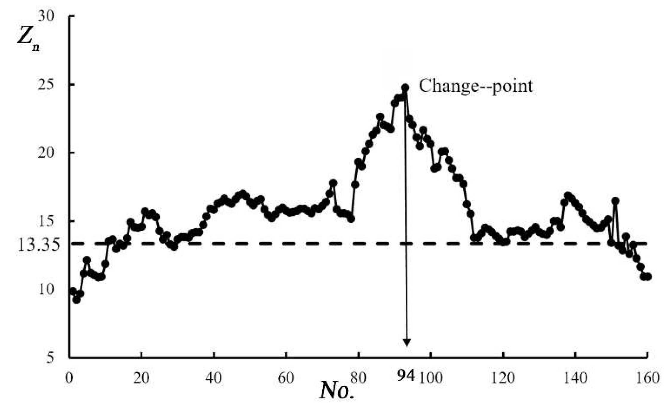
2.1.2. Test of Joint Change-Point

The purpose of testing the change-point of the multivariable dependence is to make the data more representative in different periods. At the same time, we can utilize the collected data as much as possible to improve the accuracy of the simulation.
Assuming that there is one change-point in the copula function constructed based on the observed data ( x 1 , y 1 , z 1 ) , ( x n , y n , z n ) , the original hypothesis and the alternative hypothesis can be, respectively, assumed as:
H 0 : θ 1 = θ 2 = = θ n , H 1 : θ 1 = θ n * θ n * + 1 = θ n
If the original hypothesis is rejected, then k * is the moment of change. If k * = k , the log likelihood ratio statistic of copula can be established based on the maximum likelihood estimation method, which is shown in Equation (4):
2 ln ( Λ k ) = 2 [ i = 1 k C u v w ( θ k ; U ( x i ) , V ( y i ) , W ( z i ) ) + i = k + 1 n C u v w ( θ k * ; U ( x i ) , V ( y i ) , W ( z i ) ) + i = 1 n C u v w ( θ n ; U ( x i ) , V ( y i ) , W ( z i ) ) ]
where θ k , θ k * , θ n are the maximum likelihood estimations of the corresponding data; and, C u v w ( U ( x ) , V ( y ) , W ( z ) ) = u v w C ( u , v , w ) .
The statistic Z n = max 1 k < n ( 2 ln ( Λ k ) ) is constructed. If k * is unknown, the original hypothesis will be rejected when Z n is greater than the critical value, which essentially demonstrates that the copula function has change-points [32].

2.1.3. Exceedance Probability of Water Quality

In order to quantitatively analyze the response relationship between the discharge and water quality, according to the full probability formula and the copula functions [33,34], we can calculate the probability that the water quality indicators exceed specific values. However, discharge needs to be less than a specific value, which addresses the exceedance probability of water quality. Taking the joint probability distribution of two and three dimensions as an example, the expressions are as follows:
P U 1 U 2 = P ( U 1 u 1 , U 2 u 2 ) = F U 1 ( u 1 ) F U 1 U 2 ( u 1 , u 2 )     = F U 1 ( u 1 ) C ( u 1 , u 2 )
P U 1 U 2 U 3 = P ( U 1 u 1 , U 2 u 2 , U 3 u 3 ) = F U 1 ( u 1 ) F U 1 U 2 ( u 1 , u 2 ) F U 1 U 3 ( u 1 , u 3 ) + F U 1 U U 2 3 ( u 1 , u 2 , u 3 ) = F U 1 ( u 1 ) C ( u 1 , u 2 ) C ( u 1 , u 3 ) + C ( u 1 , u 2 , u 3 )
where P U 1 U 2 is the value of the bivariate joint probability distribution; P U 1 U 2 U 3 is the value of the trivariate joint probability distribution; U 1 is the discharge; U 2 and U 3 are the water quality indicators; F U i ( u i ) is the marginal distribution function of U 1 ; and, C ( u 1 , , u i ) is the copula function of pair ( U 1 , , U i ) .

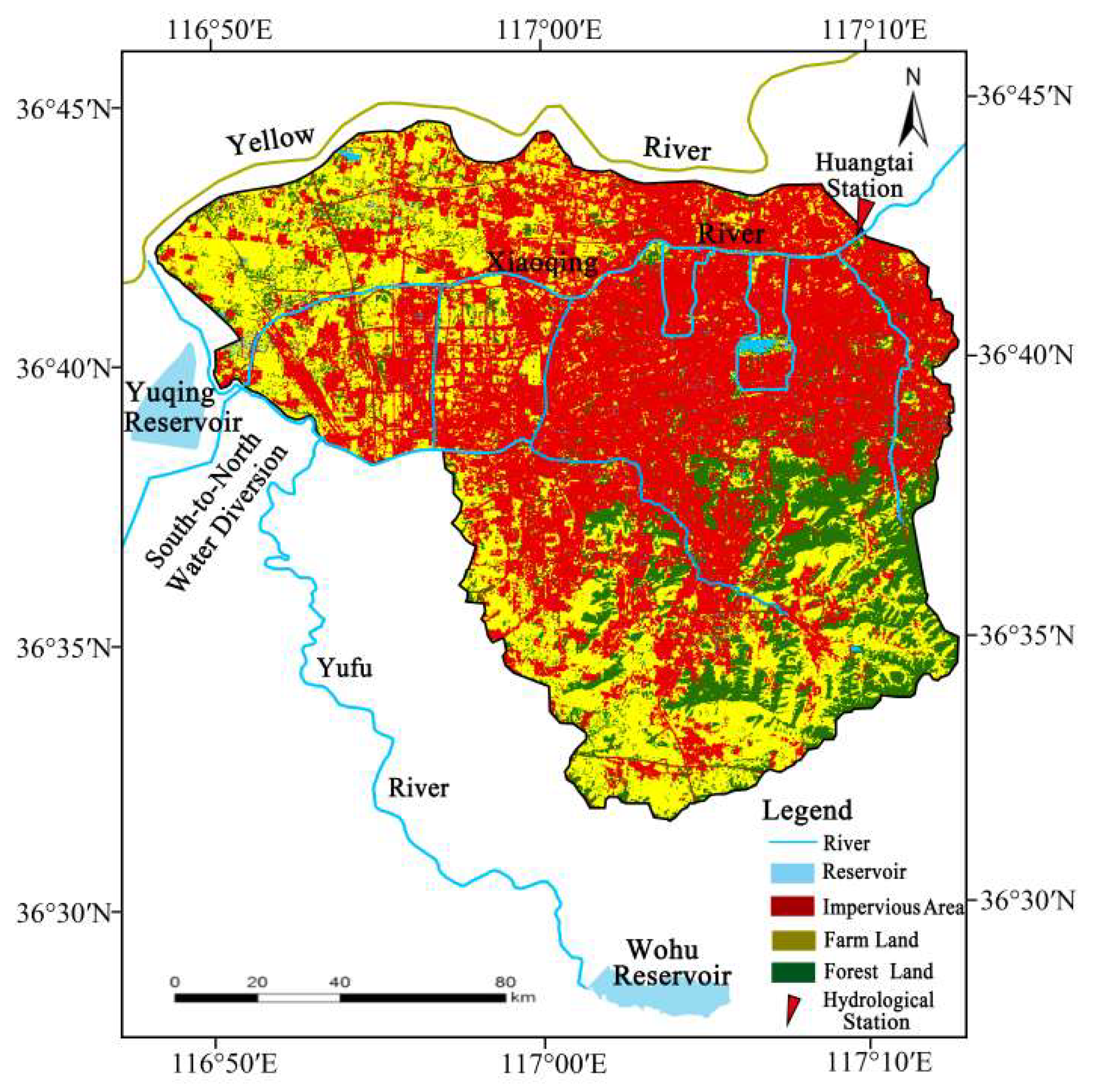
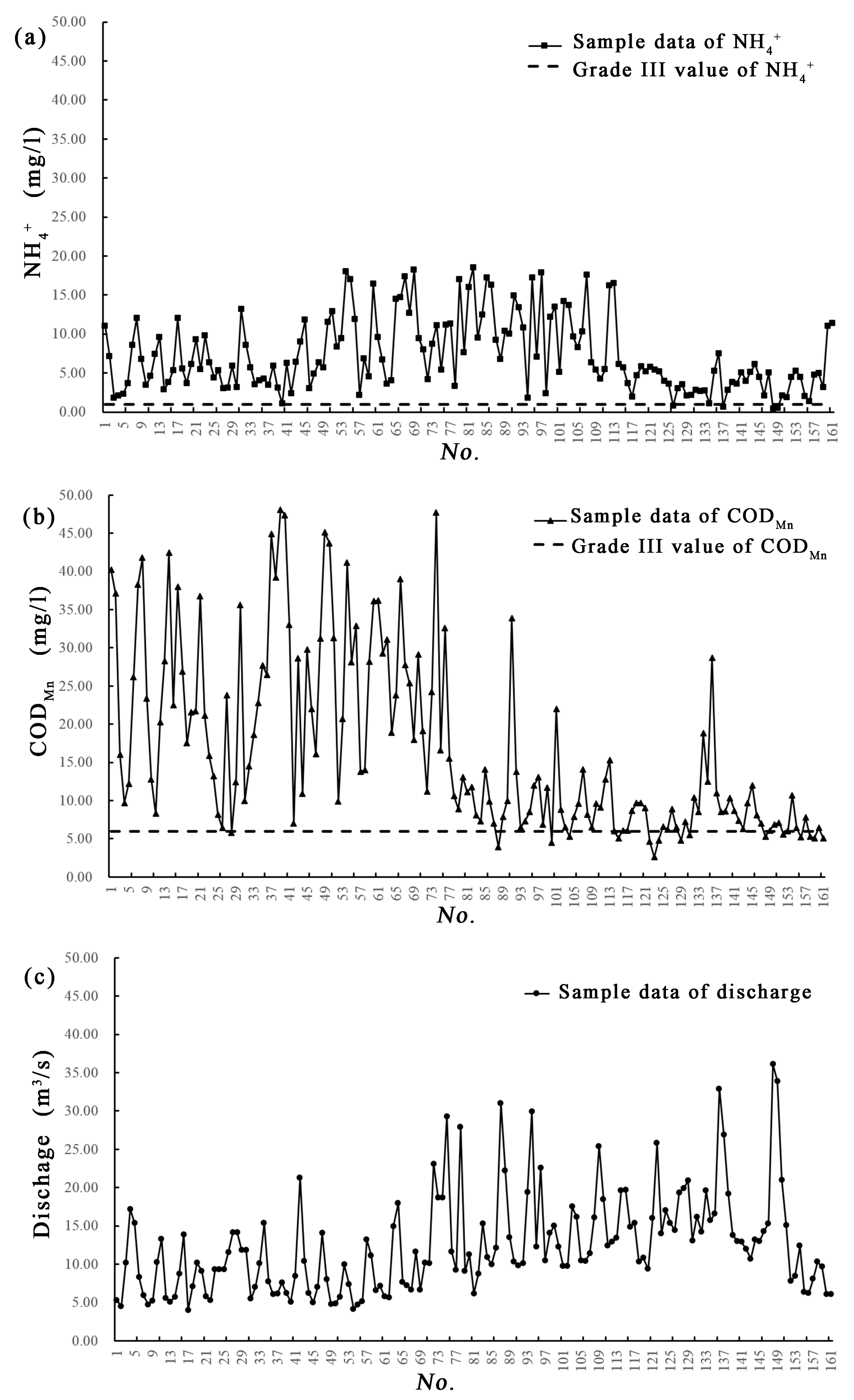
2.2. Study Area and Data

Xiaoqing River, which is located in Jinan, is a manually excavated city river. Furthermore, it is the main flood discharge channel in Jinan. The Huangtaiqiao hydrologic station is located in the main stream of the river, which has monitored the discharge from the river since 1953 with complete water quality monitoring having begun in 1970. The distance between the Muli Gate to Huangtaiqiao hydrologic station is 21.0 km, with a drainage area of 321.0 km2 and an average annual discharge of 10.4 m3/s. The river basin is located in the main urban area of Jinan. Due to the rapid development of urbanization, the water pollution in this area is serious. In order to build the ecological civilization, there has been water diversion from the Eastern Route of South-to-North Water Transfer Project to improve the water quality. However, the combined effect of urbanization and water diversion result in the response relationship between the water quantity and quality in Xiaoqing River has been severely disturbed, which has seriously affected its water quality simulation. Therefore, the statistical analysis of the occurrence probability of the combined events of water quantity and water quality can provide a basis for the scientific dispatch. The drainage map of Xiaoqing River in Jinan can be seen in Figure 1.
This study selected the data of discharge and water quality of Huangtaiqiao station during 1980–2016, with the data of water quality having been recorded every other month and the discharge having been recorded at the same time when the water quality samples were taken (using the main pollutants, nitrogen content index (NH4+), which includes the ionised ammonia nitrogen and the free ammonia nitrogen, and permanganate index (CODMn) as the calculation indicators). To remove some unreasonable data, 161 sets of water quantity and water quality data were applied in this paper. The sample data series of NH4+, CODMn, and discharge of the Huangtai Station from 1980 to 2016 are shown in Figure 2, and the characteristics and trend results of the generalized basic data about the water quality are given in Table 1. The trends of the generalized basic data are tested by Mann-Kendall (M-K). It can be seen that the concentrations of NH4+ and CODMn are basically larger than the grade III value (Environmental Quality Standards for Surface Water (GB3838-2002)). Moreover, the CODMn has a significant decreasing trend, and the discharge has a significant increasing trend, while the trend of NH4+ descending was not obvious.
In order to better reflect the relationship between the discharge and the multiple water quality indicators in the Xiaoqing River Basin, which is a rapidly developing area, we carried out a test for the change-point of the long sequence data (1980–2016), before focusing on the analysis of the data after the change-point.

3. Results and Discussion

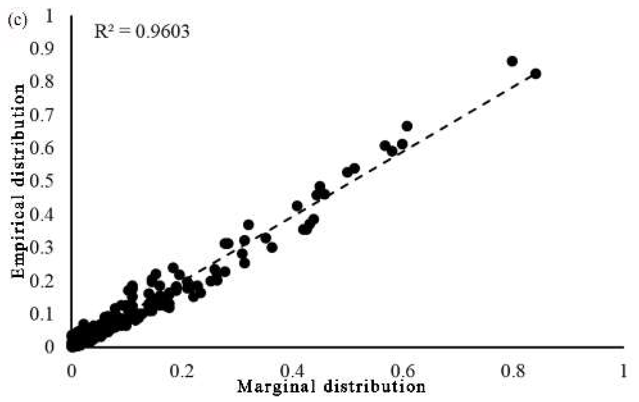
3.1. Marginal Distributions and Correlation Coefficient of Q, NH4+ and CODMn

The marginal distributions of the Q, NH4+, and CODMn of Xiaoqing River are established by the lognormal, gamma, and Pearson-III distributions to search for the proper cumulative distribution function (CDF). The proper CDF of the parameters was chosen using two goodness fit tests: the Kolmogorov–Smirov (K–S) test and root mean squared error (RMSE) test. The results of the proper marginal distribution of each variable are shown in Table 2. From Table 2, we can see that the marginal distribution of Q and NH4+ sequence is more consistent with a Gamma distribution, while CODMn is more consistent with a lognormal distribution.
The Kendall correlation coefficient τ is used to analyze the correlation of Q, NH4+, and CODMn, respectively, which is shown in Table 3. We can see that the pair of (Q, NH4+) and the pair of (Q, CODMn) are negatively correlated, while the pair (NH4+, CODMn) has a positive correlation. This provides the conditions for the application of Gaussian Copula.

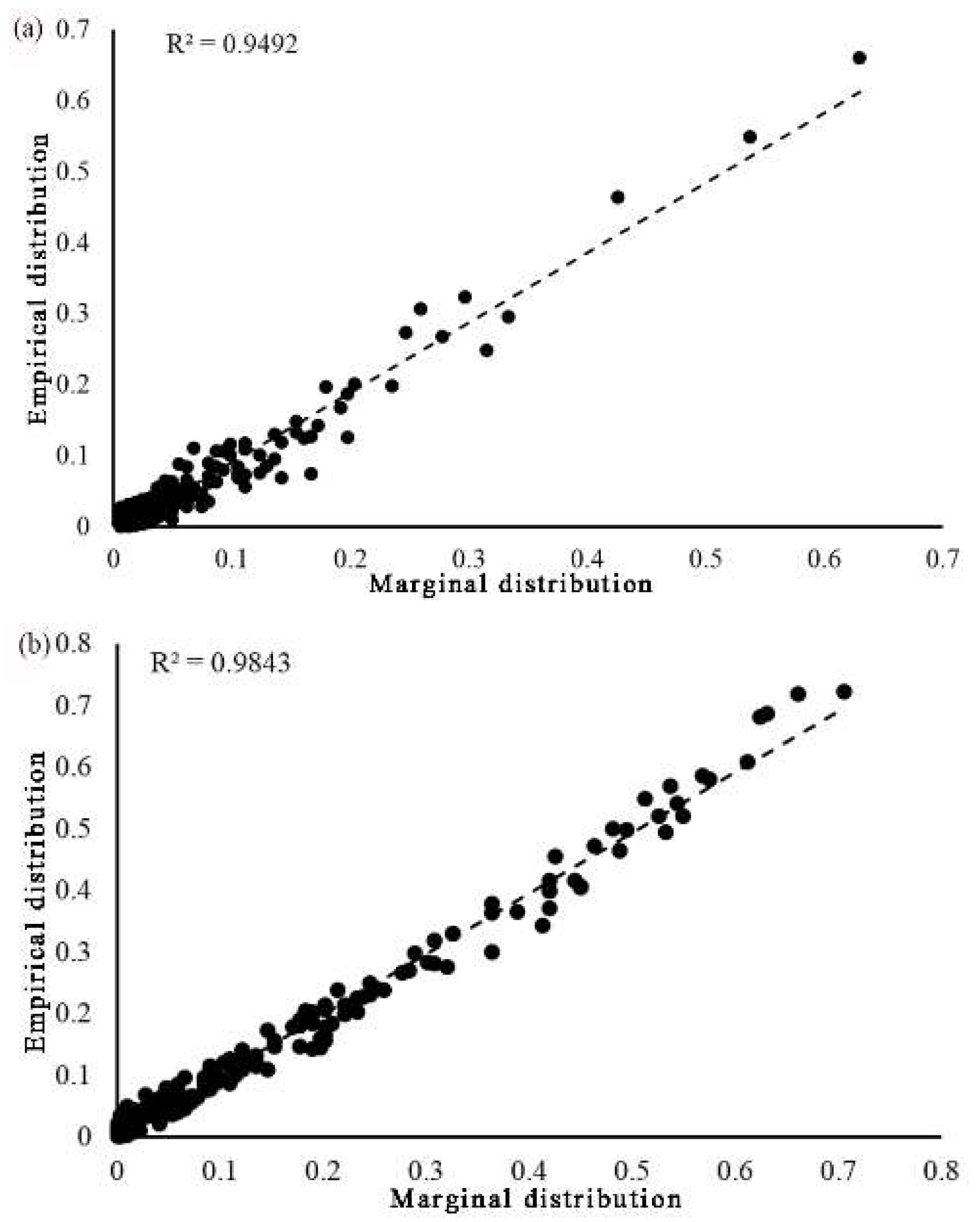
3.2. Establishment of Joint Probability Distribution

3.2.1. Establishment of Multivariate Joint Probability Distribution of Q, NH4+, and CODMn with the Data from 1980–2016

The Frank, GH, and Gaussian copulas are used to construct the bivariate and trivariate joint probability distributions with the data of water quantity and water quality of Xiaoqing River in Jinan that were obtained during 1980–2016. The proper distribution was chosen using K–S and the RMSE tests, with the parameters of copulas and the results of the goodness fit being shown in Table 4. Figure 3 compares the sample empirical distribution with the joint distribution of the pairs of (Q, NH4+), (Q, CODMn), and (Q, NH4+, CODMn). From these figures, we can see that the correlation coefficients R2 of Gaussian copula are higher. This illustrates that the Gaussian copula is more suitable in establishing both the bivariate joint probability distributions and the trivariate joint probability distribution.

3.2.2. Test of Joint Change-Point of Q, NH4+, and CODMn

According to the optimal fitting copula functions of Q, NH4+, and CODMn using the data from 1980–2016, the joint change-points can be identified. When the number of data is 161, the critical value of Z n is 13.35 [35]. The results are shown in Figure 4, which show that Z n is greater than its critical value in No. 94 of the data, which is July 2005. Therefore, this is the change-point of the combination of (Q, NH4+, CODMn). Furthermore, the result also matches the actual situation: the continuous drought for several years before 2005 in Jinan resulted in the management department transferring about 1 × 10⁸ m3 of water into the Xiaoqing River, which might cause a change in the relationship between the water quantity and quality.
This indicates that the dependency relationship of the data was inconsistent between 1980 and 2016, so a change-point test was needed to identify the data sequences that are consistent with the current situation.

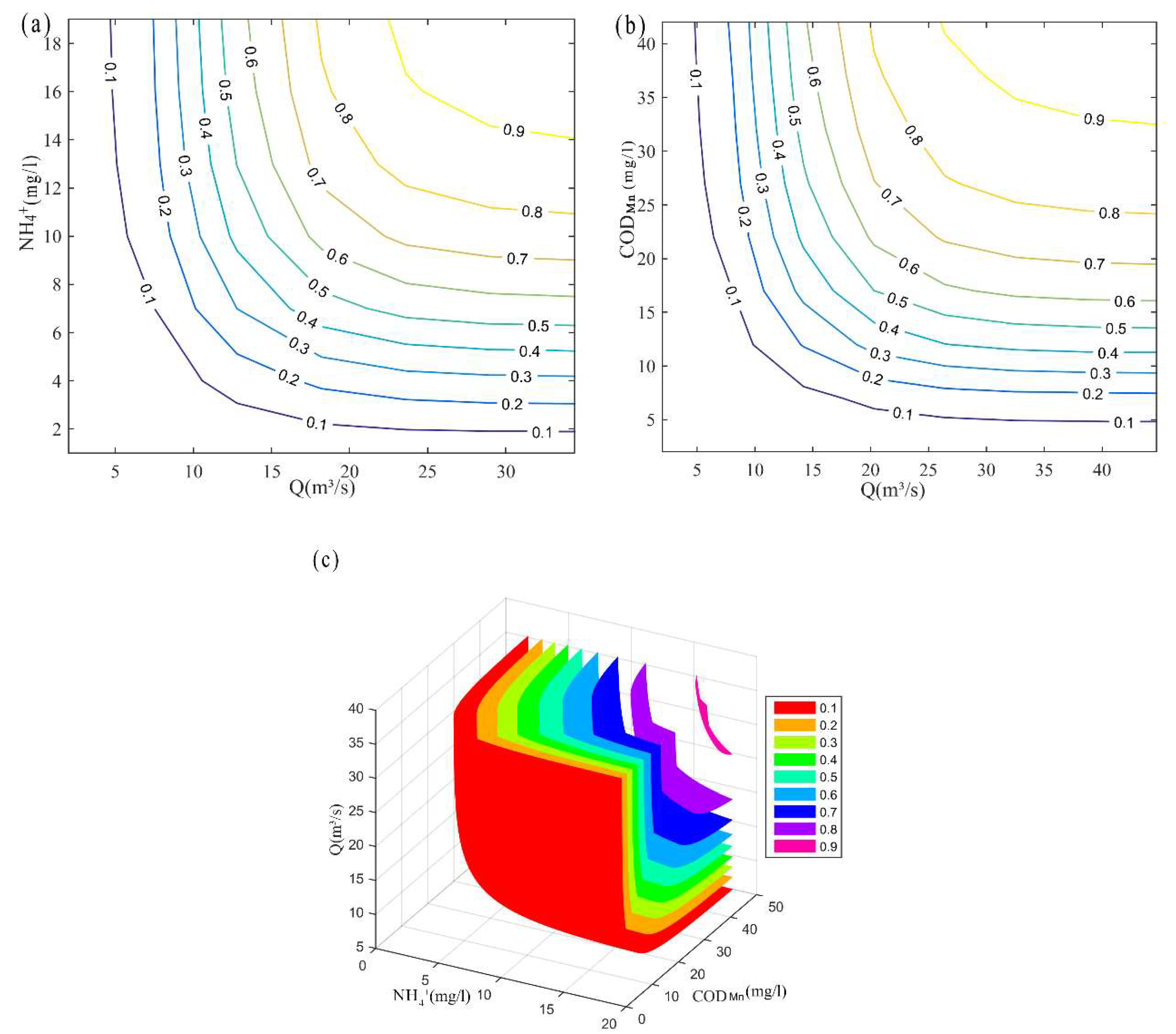
3.2.3. Establishment of Multivariate Joint Probability Distribution after the Joint Change-Point

The data of Q, NH4+, and CODMn after the joint change-point is more representative of the relationship between water quantity and quality in recent years. Therefore, we re-established the multivariate joint probability distribution using the data after the change-point. The parameters of the copulas and the results of the goodness fit are shown in Table 5. From Table 5, we can see that the joint probability distributions are still consistent with the Gaussian copula function. Meanwhile, their corresponding contour plots and contour surface are presented in Figure 5.

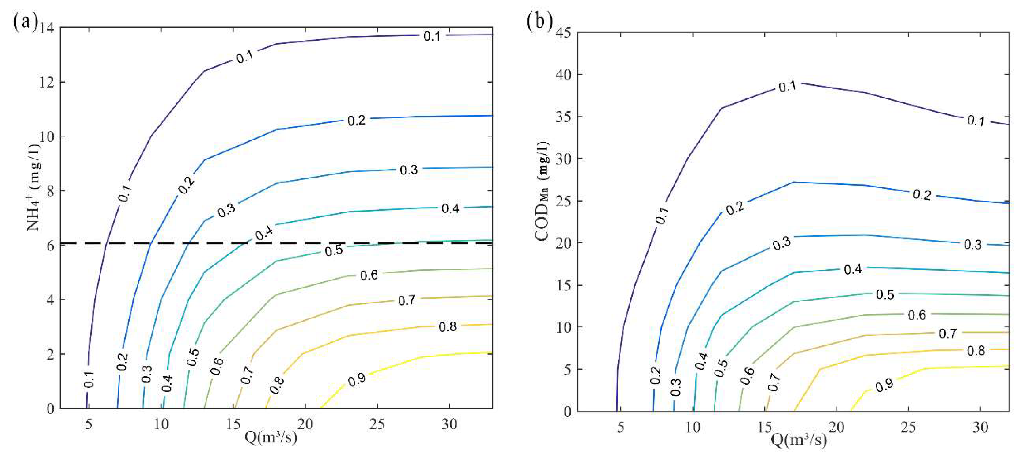
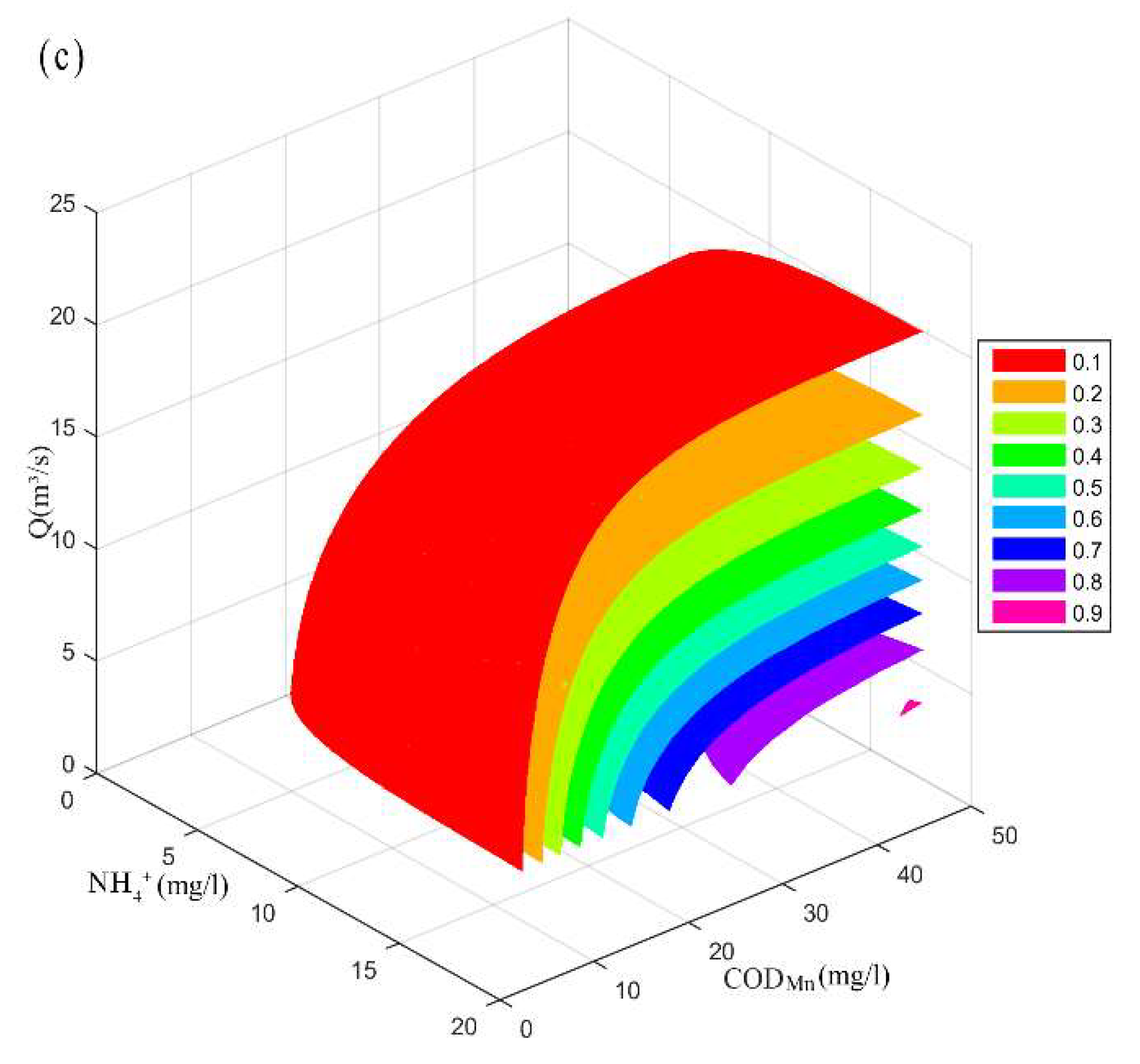
3.3. Analysis of Multivariate Joint Probability Distribution of Q, NH4+ and CODMn after the Joint Change-Point

According to the real situation of the river water quality and the existing water quality standards “Environmental Quality Standards for Surface Water” (GB3838-2002), we conducted a cluster analysis of the water quality to obtain the new classes of water quality, which are shown in Table 6.
Using the constructed joint probability distribution of Q, NH4+, and CODMn, the probability of the water quality exceeding a specific value under the different conditions of discharge can be analyzed by Equations (3) and (4). P U 1 U 2 and P U 1 U 3 are the bivariate joint probability distributions of the pair of (Q, NH4+) and the pair of (Q, CODMn), respectively, which represent the exceedance probability of NH4+ or CODMn in different discharge situations. P U 1 U U 2 3 is the trivariate joint probability distribution of the pair of (Q, NH4+, CODMn), which represents the combined exceedance probability of (NH4+, CODMn) in different discharge situations. The contour plots of P U 1 U 2 and P U 1 U 3 are given in Figure 6a,b, respectively, while the contour surface of P U 1 U U 2 3 is shown in Figure 6c.
From Figure 6a,b, we can see that when P U 1 U 2 or P U 1 U 3 is in the range of 0.1–0.4, the contour plot is relatively sparse, especially in the upper right panel of the figures. This indicates that when the concentration of NH4+ or CODMn is high, the joint probability is insensitive to a change in discharge. For the combination of NH4+ and CODMn, Figure 6c shows that, when P U 1 U U 2 3 is between 0.1–0.3, the contour surface is relatively sparse. This is mainly due to the large amount of pollutants in the water body of Xiaoqing River at this moment. At the same time, the tributaries also carry pollutants so the joint probability is insensitive to a change in the discharge.
The typical values of the joint probability of Q, NH4+, and CODMn are given in Table 7, Table 8 and Table 9, which describe the probability of the water quality indicators exceeding the specific values with different combinations of discharge and water quality indicators. For example, under the condition that only NH4+ is considered, P U 1 U 2 = P ( U 1 12 , U 2 6.3 ) = 0.1985 . Under the condition that only CODMn is considered, P U 1 U 3 = P ( U 1 12 , U 3 12.0 ) = 0.2135 . Finally, under the condition that NH4+ and CODMn are synergistically considered, P U 1 U U 2 3 = P ( U 1 12 , U 2 6.3 , U 3 12.0 ) = 0.2493 . The results show that the trivariate joint probability of the combination of (Q, NH4+, CODMn) is larger than the bivariate joint probability of the pairs of (Q, NH4+) and (Q, CODMn). This indicates that the probability of exceeding the standards of multiple indicators is greater than that of exceeding individual indicators, which is more consistent with the actual situation. Therefore, only considering the discharge and individual water quality indicator cannot reasonably reflect the relationship between the discharge and water quality. The trivariate joint probability distribution considering Q, NH4+, and CODMn can more comprehensively express the characteristics of discharge and multiple water quality indicators.

3.4. Discussion

There is not always a positive correlation between the discharge and water quality indicators, which means that the correlation between variables is asymmetric. In this paper, although Frank and G-H Copulas, which are symmetric copula functions, can fit the probability distribution between the discharge and water quality, the fitting accuracy, and the simulation of higher dimensions are not sufficient when compared to the asymmetric Gaussian copulas. Based on the statistical analysis of the historical data of discharge and water quality, this paper provides a method to quantitatively evaluate the exceedance probability of water quality by considering the joint probability of Q, NH4+, and CODMn. When compared with the previous non-mechanical methods, this method adopts a multi-dimensional joint distribution that is based on a copula to more accurately describe the response relationship between water quality and discharge under the condition of the coexistence of multiple pollutants in rivers.
The trivariate joint probability distribution of the combination of (Q, NH4+, CODMn) can reflect the joint probability for the different combinations of Q, NH4+, and CODMn. Thus, when the combination events (NH4+, CODMn) exceed their given design values in different discharge situations, the exceedance probability can be calculated. Generally, regardless of whether the pollutant is NH4+, CODMn, or a combination of NH4+ and CODMn, the joint probability tends to increase with an increase in the discharge and a decrease in the concentration of pollutants discharged into rivers. Thus, the exceedance probability of the water quality can be reduced by an increase in discharge (Q) and a decrease in concentration of pollutants (NH4+ and CODMn). However, with an increase in discharge, the counter lines or the counter surface tend to level, which means that there is a limit imposed on the improvement of water quality. Therefore, further research is needed to determine the limit value. In addition, we suggest that the administration should strengthen the monitoring of water quality at each entry section of Xiaoqing River so that we can obtain a more comprehensive relationship between the discharge and water quality.

4. Conclusions

In this paper, the joint probability distributions of discharge and the main pollutants of NH4+ and CODMn of Xiaoqing River in Jinan were constructed by copulas, before the exceedance probability of water quality combination events under different discharge conditions was analyzed. The specific conclusions are as follows:
(1)
The Gaussian copula is more suitable for describing the multivariate joint probability distribution of discharge and water quality. As the relationship between the discharge and water quality indicators is not always positive, the Gaussian copula is more suitable than the Archimedean copulas in the simulation of trivariate or the above joint distribution.
(2)
Based on the copula, the joint change-point can be identified. For urban rivers, the dependence of water quantity and quality is often affected by human activities, which leads to the emergence of change-point. Therefore, it is necessary to identify the mutation points.
(3)
The trivariate joint probability distribution of the combination of (Q, NH4+, CODMn) is more suitable for estimating the various exceedance probability of the water quality effectively under different discharge conditions. Thus, when the combination events (NH4+, CODMn) exceed their given values in the specific discharge situation, the exceedance probability can be calculated.

Author Contributions

Y.L. and X.Z. collected and analyzed the data; Y.C. and X.L. performed the collation of figures and tables; S.C. contributed analysis tools; Y.L. carried out calculation and completed the manuscript.

Funding

This study was funded by the Special Scientific Research Fund of Public Welfare Profession of Ministry of Water Resources of China: Key Technology Research and Demonstration Project of Water Ecological Civilization Construction (No. 201401003) and the Shandong Provincial Water Conservancy Scientific Research and Technology Promotion Project (No. SDSLKY201302).

Conflicts of Interest

The authors declare no conflict of interest. The founding sponsors had no role in the design of the study; in the collection, analyses, or interpretation of data; in the writing of the manuscript, and in the decision to publish the results.

References

  1. Jang, C.S.; Chen, S.K.; Kuo, Y.M. Establishing an irrigation management plan of sustainable groundwater based on spatial variability of water quality and quantity. J. Hydrol. 2012, 414, 201–210. [Google Scholar] [CrossRef]
  2. Qian, L.; Liu, Y.; Chao, J.Y. The current situation and development trend of China joint regulating of water quality and water quantity. Environ. Sci. Technol. 2013, 36, 484–487. [Google Scholar] [CrossRef]
  3. Shokri, A.; Haddad, O.B.; Mariño, M.A. Multi-objective quantity-quality reservoir operation in sudden pollution. Water Resour. Manag. 2014, 28, 567–586. [Google Scholar] [CrossRef]
  4. Zhang, M.N.; Dolatshah, A.; Zhu, W.L.; Yu, G.L. Case Study on Water Quality Improvement in Xihu Lake through Diversion and Water Distribution. Water 2018, 10, 333. [Google Scholar] [CrossRef]
  5. Zhang, X.; Ran, Q.X.; Xia, J.; Song, X.Y. Jointed distribution function of water quality and water quantity based on Copula. J. Hydraul. Eng. 2011, 42, 483–489. [Google Scholar] [CrossRef]
  6. Cox, B.A. A review of currently available in-stream water-quality models and their applicability for simulating dissolved oxygen in lowland rivers. Sci. Total. Environ. 2003, 314–316, 335–377. [Google Scholar] [CrossRef]
  7. Wang, S.W.; Qi, S.Q.; Yu, D.D.; Zhang, Y.W.; Wan, L.H. Forecast and evaluation of water environment quality based on WASP model: A case study on Harbin section of Songhua River. J. Nat. Disast. 2015, 24, 39–45. [Google Scholar] [CrossRef]
  8. Yu, S.; He, L.; Lu, H.W. An environmental fairness based optimisation model for the decision-support of joint control over the water quantity and quality of a river basin. J. Hydrol. 2016, 535, 366–376. [Google Scholar] [CrossRef]
  9. Phan, T.D.; Smart, J.C.R.; Capon, S.J.; Hadwen, W.L.; Sahin, O. Applications of Bayesian belief networks in water resource management. Environ. Model. Softw. 2016, 85, 98–111. [Google Scholar] [CrossRef]
  10. Yang, B.; Lai, C.G.; Chen, X.H.; Wu, X.Q.; He, Y.H. Surface water quality evaluation based on a Game Theory-Based Cloud model. Water 2018, 10, 510. [Google Scholar] [CrossRef]
  11. Jia, H.; Xu, T.; Liang, S.; Zhao, P.; Xu, C. Bayesian framework of parameter sensitivity, uncertainty, and identifiability analysis in complex water quality models. Environ. Model. Softw. 2018, 104, 13–26. [Google Scholar] [CrossRef]
  12. Sun, Z.B.; Wang, B.L.; Ji, H.F.; Huang, Z.Y.; Li, H.Q. Water quality prediction based on probability-combination. China Environ. Sci. 2011, 31, 1657–1662. [Google Scholar]
  13. Junyi, N.; Hu, H.; Na, C. Combined risk prediction in the water environment based on an MS-AR model and copula theory. WST 2013, 67, 1967. [Google Scholar] [CrossRef] [PubMed]
  14. Parmar, K.S.; Bhardwaj, R. River water prediction modeling using neural networks, fuzzy and wavelet coupled model. Water Resour. Manag. 2015, 29, 17–33. [Google Scholar] [CrossRef]
  15. Zhao, F.; Li, C.H.; Chen, L.B.; Zhang, Y. An integrated method for accounting for water environmental capacity of the River–Reservoir combination system. Water 2018, 10, 483. [Google Scholar] [CrossRef]
  16. Wang, G.; Wang, S.; Kang, Q.; Duan, H.; Wang, X. An integrated model for simulating and diagnosing the water quality based on the system dynamics and Bayesian network. WST 2016, 74, 2639. [Google Scholar] [CrossRef] [PubMed]
  17. Barzegar, R.; Adamowski, J.; Moghaddam, A.A. Application of wavelet-artificial intelligence hybrid models for water quality prediction: A case study in Aji-Chay River, Iran. Stoch. Environ. Res. Risk A 2016, 30, 1–23. [Google Scholar] [CrossRef]
  18. Chowdhary, H.; Escobar, L.A.; Singh, V.P. Identification of suitable copulas for bivariate frequency analysis of flood peak and flood volume data. Hydrol. Res. 2011, 42, 193–216. [Google Scholar] [CrossRef]
  19. Bezak, N.; Mikoš, M.; Šraj, M. Trivariate frequency analyses of peak discharge, hydrograph volume and suspended sediment concentration data using copulas. Water Resour. Manag. 2014, 28, 2195–2212. [Google Scholar] [CrossRef]
  20. Fontanazza, C.M.; Freni, G.; La, L.G.; Notaro, V. Uncertainty evaluation of design rainfall for urban flood risk analysis. WST 2011, 63, 2641–2650. [Google Scholar] [CrossRef]
  21. Luca, D.L.D.; Biondi, D. Bivariate return period for design hyetograph and relationship with T-Year design flood peak. Water 2018, 9, 673. [Google Scholar] [CrossRef]
  22. Guo, S.L.; Muhammad, R.; Liu, Z.J.; Xiong, F.; Yin, J.B. Design flood estimation methods for Cascade Reservoirs based on Copulas. Water 2018, 10, 560. [Google Scholar] [CrossRef]
  23. Bazrafshan, J.; Nadi, M.; Ghorbani, K. Comparison of empirical copula-based joint deficit index (JDI) and multivariate standardized precipitation index (MSPI) for drought monitoring in Iran. Water Resour. Manag. 2015, 29, 2027–2044. [Google Scholar] [CrossRef]
  24. Salvadori, G.; Michele, C.D. Multivariate real-time assessment of droughts via copula-based multisite Hazard Trajectories and Fans. J. Hydrol. 2015, 526, 101–115. [Google Scholar] [CrossRef]
  25. Katipoğlu, O.M.; Can, İ. Determining the lengths of dry periods in annual and monthly stream flows using runs analysis at Karasu River, in Turkey. WST 2017, 18. [Google Scholar] [CrossRef]
  26. Li, Y.; Chen, C.; Sun, C. Drought severity and change in Xinjiang, China, over 1961–2013. Hydrol. Res. 2017, 48, 1343–1362. [Google Scholar] [CrossRef]
  27. Muhammad, A.; Maeng, S.J.; San Kim, H.; Murtazaev, A. Copula-Based stochastic simulation for regional drought risk assessment in South Korea. Water 2018, 10, 359. [Google Scholar] [CrossRef]
  28. Jaewon, K.; Kim, S.; Kim, G.; Singh, V.P.; Park, J.; Kim, H.S. Bivariate drought analysis using streamflow reconstruction with Tree Ring Indices in the Sacramento Basin, California, USA. Water 2016, 8, 122. [Google Scholar] [CrossRef]
  29. Sklar, A. Fonctions de rèpartition à n dimensions et leurs marges. Publ. Inst. Stat. Univ. Paris 1959, 8, 229–231. [Google Scholar]
  30. Wang, Y.; Li, C.Z.; Liu, J.; Yu, F.L.; Qiu, Q.T.; Tian, J.Y.; Zhang, M.J. Multivariate Analysis of Joint Probability of Different Rainfall Frequencies Based on Copulas. Water 2017, 9, 198. [Google Scholar] [CrossRef]
  31. Genest, C.; Favre, A.C.; Béliveau, J.; Jacques, C. Metaelliptical copulas and their use in frequency analysis of multivariate hydrological data. Water Resour. Res. 2007, 43, 223–236. [Google Scholar] [CrossRef]
  32. Guo, A.; Qiang, H.; Wang, Y.; Li, Y.; Chang, J.; Mo, S. Detection of variations in precipitation-runoff relationship based on archimedean copula. J. Hydroelectr. Eng. 2015, 34, 7–13. [Google Scholar]
  33. Fan, Y.R.; Huang, W.W.; Huang, G.H.; Li, Y.P.; Huang, K.; Li, Z. Hydrologic risk analysis in the Yangtze River basin through coupling Gaussian mixtures into copulas. Adv. Water Resour. 2016, 88, 170–185. [Google Scholar] [CrossRef]
  34. Song, S.B.; Nie, R. Asymmetric Archimedean Copulas for multivariate hydrological drought frequency analysis. J. Hydroelectr. Eng. 2011, 30, 20–29. [Google Scholar]
  35. Dias, A.D.C. Copula Inference for Finance and Insurance. Ph.D. Thesis, Swiss Federal Institute of Technology Zurich, Zurich, Swiss, 2004. [Google Scholar]
Figure 1. Location of Xiaoqing River in Jinan and drainage map.
Water 10 00971 g001
Figure 2. The data series of nitrogen content index (NH4+), permanganate index (CODMn), and discharge of the Huangtai Station from 1980 to 2016: (a) the sample data and grade III value of NH4+ ; (b) the sample data and grade III value of CODMn; and, (c) the sample data of discharge.
Water 10 00971 g002
Figure 3. Comparison of the sample empirical distribution and marginal distribution: (a) pair of (Q, NH4+); (b) pair of (Q, CODMn); and, (c) pair of (Q, NH4+, CODMn).
Water 10 00971 g003aWater 10 00971 g003b
Figure 4. Analysis of the joint change-points of the combination of (Q, NH4+, CODMn).
Water 10 00971 g004
Figure 5. The contour plots and contour surface: (a) bivariate joint probability of (Q, NH4+); (b) bivariate joint probability of (Q, CODMn); and, (c) trivariate joint probability of the combination of (Q, NH4+, CODMn).
Water 10 00971 g005
Figure 6. The contour plots and contour surface: (a) P U 1 U 2 ; (b) P U 1 U 3 ; and, (c) P U 1 U U 2 3 .
Water 10 00971 g006aWater 10 00971 g006b
Table 1. The trend results of NH4+, CODMn, and discharge.
NH4+ (mg/L)CODMn (mg/L)Discharge (m3/s)Water Temperature (°C)pH
Minimum0.432.603.9935.50
Maximum18.5048.1036.103111.60
Mean7.2316.8612.4318.947.51
Trend++
Note: means a decreasing trend; means a raising trend; + means significant trend; means non-significant trend.
Table 2. The parameters of marginal distributions of Q, NH4+, and CODMn and results of Kolmogorov–Smirov (K–S) and root mean squared error (RMSE).
Lognormal Gamma Pearson III
( μ , σ )KSRMSE ( μ , σ )KSRMSE ( μ , σ , α 0 )KSRMSE
Q2.398, 0.4940.0570.0284.255, 2.9210.0510.0210.553, 23.406, −0.5080.4310.228
NH4+1.738, 0.7510.1520.0262.238, 3.2300.0630.0222.367, 3.149, −0.2220.0660.028
CODMn2.588, 0.6900.0720.0532.266, 7.4400.1210.0671.470, 10.291, 1.7370.0970.055
Note: The number in bold means that RSME is the minimum and the K–S is 0.10172 according to the 5% significance level when n = 161.
Table 3. The correlation coefficient τ of Q, NH4+, and CODMn.
PairQ, NH4+Q, CODMnNH4+, CODMn
τ −0.2712−0.39920.1933
Table 4. The parameters of copulas of Q, NH4+, and CODMn, and results of K–S and RMSE.
PairsParametersK–SRMSE
FrankQ, NH4+ θ = 0.6114 0.10320.0541
Q, CODMn θ = 0.5890 0.08670.0353
Q, NH4+, CODMn θ = 0.9315 0.10780.0331
GHQ, NH4+ θ = 0.7866 0.08420.0251
Q, CODMn θ = 0.7147 0.08920.0337
Q, NH4+, CODMn θ = 0.9236 0.10030.0343
GaussianQ, NH4+ ρ = 0.4036 0.08120.0251
Q, CODMn ρ = 0.5319 0.07520.0323
Q, NH4+, CODMn ρ 12 = 0.4036 ρ 13 = 0.5319 ρ 23 = 0.2645 0.09060.0222
Note: ρ 12 is the correlation coefficient of (Q, NH4+); ρ 13 is the correlation coefficient of (Q, CODMn); and ρ 23 is the correlation coefficient of (NH4+, CODMn). The K–S is 0.1626 according to the 5% significance level when n = 70.
Table 5. The parameters of copulas of Q, NH4+, and CODMn and the results of K–S and RMSE.
PairsParametersK–SRMSE
FrankQ, NH4+ θ = 0.5869 0.16670.0654
Q, CODMn θ = 0.5971 0.15460.0621
Q, NH4+, CODMn θ = 0.2998 0.18160.0651
GHQ, NH4+ θ = 0.8295 0.21360.0711
Q, CODMn θ = 0.9509 0.20950.0604
Q, NH4+, CODMn θ = 2.8152 0.17910.0743
GaussianQ, NH4+ ρ = 0.4073 0.14310.0462
Q, CODMn ρ = 0.4037 0.13150.0493
Q, NH4+, CODMn ρ 12 = 0.4073 ρ 13 = 0.4037 ρ 23 = 0.4151 0.11630.0524
Table 6. Classes of water quality for NH4+ and CODMn.
Cluster CenterBoundary Values
Center 1Center 2Center 3Center 4Class 1Class 2Class 3Class 4Class 5
NH4+4.26.38.511.2<4.24.2~6.36.3~8.58.5~11.2>11.2
CODMn8.012.024.035.0<8.08.0~12.012.0~24.024.0~35.0>35.0
Table 7. The typical values of exceedance probability of NH4+.
NH4+Q(m3/s)
(mg/L)36122436
4.20.01330.06530.25890.40790.4177
6.30.01200.05520.19850.29160.2964
8.5---0.04260.13790.19000.1921
11.2---0.02870.08270.10700.1078
Note: “---” denotes impossible events.
Table 8. The typical values of exceedance probability of CODMn.
CODMnQ(m3/s)
(mg/L)36122436
8.00.01350.06450.26380.41470.4231
12.00.01340.05870.21350.30430.3077
24.0---0.03410.08960.10770.1080
35.0---0.01840.03950.04430.0443
Note: “---” denotes impossible events.
Table 9. The typical values of combined exceedance probability of NH4+ and CODMn.
NH4+CODMnQ(m3/s)
(mg/L)(mg/L)36122436
4.280.01380.10560.38970.55960.5658
120.01280.09640.31940.42440.4270
240.00960.05660.13870.16070.1609
350.00640.03080.06250.06850.0685
6.380.01200.08940.30110.40940.4125
120.01160.08190.24930.31730.3187
240.00880.04870.11160.12630.1264
350.00590.02680.05140.05540.0554
8.580.01010.06910.21080.27250.2740
120.00980.06350.17660.21590.2165
24---0.03840.08180.09050.0906
35---0.02140.03860.04110.0411
11.28---0.04670.12750.15690.1575
12---0.04320.10820.12720.1274
24------0.05220.05650.0566
35------0.02540.02660.0266
Note: “---” denotes impossible events.

