1. Introduction
Groundwater is an important water resource and a major factor for maintaining the regional ecological environment, which plays a significant role in ensuring water, food, economic, and ecological security [
1,
2]. In the past few years, groundwater has become the main source of agricultural irrigation because of the wide range of distribution and convenient access [
3]. The continuous extraction of groundwater every year will not only cause a decline of the local groundwater level, but also will change the local hydrological cycle and energy cycle, which will eventually affect regional climate [
4,
5,
6,
7,
8]. At the same time, groundwater depletion will also affect the sustainability of food production, and food and water security locally and globally through the international food trade [
9,
10]. The groundwater overdraft has caused global groundwater to be exhausted at an alarming rate [
11,
12,
13], especially in key food-producing regions, such as the North China Plain, the central USA and California, and north-western India [
9,
10,
14]. The status mentioned above has been located and quantified by both hydrological modelling [
11] and Earth observations [
9,
12]. As groundwater is mainly extracted by electric pumps, excessive exploitation of groundwater will increase electricity consumption, thus increasing the global carbon emissions [
15]. The increase in carbon emissions not only affects global climate change, but also has a huge impact on the global economy [
16]. Therefore, the problem brought about by groundwater overdraft is a global issue.
Hebei Province is the main grain-producing area of China [
17]. Because of a surface water shortage, groundwater is the main source for industry and agriculture. With socio-economic development, the groundwater overdraft in Hebei Province began in the 1970s [
18]. The annual average overdraft amount is up to 5.965 billion m
3. The Hebei plain area became one of the areas with the highest degree of groundwater exploitation and utilization in China [
19]. The long-term excessive exploitation of groundwater has caused a continuous decline in groundwater depth [
19]. Combined with the influence of human activities and climate change, it has caused a series of geological and groundwater ecological environment problems, such as the deep and shallow groundwater depression cone, ground subsidence, and the migration of the salt and fresh water interface [
19,
20]. The problems of groundwater in Hebei Province have deeply affected the healthy development of regional water resources, the ecological environment and the economy, and have threatened water and food security. Therefore, it is necessary to implement the treatment of groundwater overdraft.
As the problems of the groundwater overdraft are becoming increasingly serious, a large number of domestic and foreign scholars have gradually begun to pay attention to water resources (especially environmental and ecological aspect) and other problems caused by the groundwater overdraft. Bouwer et al. and Konikow et al. found that the depletion of groundwater can eventually lead to critical environmental degradation, such as seawater intrusion and land subsidence [
21,
22]. Hu et al. illustrated the environmental issues caused by the groundwater overdraft, such as land subsidence, ground fissure, seawater invasion, etc. [
23]. Wolff, Rothenburg et al., Holzer, and Boling have conducted research on the interaction between the groundwater overdraft and geological fractures [
24,
25,
26,
27]. Lee et al. have explored the seawater intrusion caused by groundwater overexploitation in the coastal plains of Korea [
28]. Karatzas et al. insisted that in order to control the invasion of sea water, it is necessary to control the production of pumping wells and to find new alternative water sources [
29]. Through the use of ground subsidence and depression data, the environmental problems caused by groundwater overexploitation were studied by Shi et al [
20]. The response of climate change to the groundwater overexploitation in East Asian monsoon area and the Haihe River Basin was studied by Yuan et al. [
6] and Zou et al. [
30], respectively. The overdraft of groundwater also threatens food security, and some scholars have studied this issue. Yuan et al. found the food production has a close relationship with groundwater dynamics [
31]. Through the study of the correlation of global food trade and groundwater depletion, Dalin et al. discovered that the current situation of the vast majority of the world's population depends on the importation of food, which highlights the risk of global food security and water safety. They also suggested that countries which both export and import food irrigated from fast exhausted groundwater were particularly exposed to these risks (including the USA, Mexico, Iran and China) [
32].
As China has large food imports and exports, the threat of groundwater overdraft is more serious. The Central Committee and the State Council of China announced the Central Document No. 1 in 2014. This motion encouraged researchers to “carry out the comprehensive treatment for groundwater overdraft in groundwater depression cone area in North China”. As Hebei is the most serious groundwater overdraft area in the world, the relevant ministries and commissions of the state organized the first annual comprehensive treatment project in Hebei Province to repair and improve the groundwater eco-environment. Some experts and scholars have explored the technology and measures to solve the problems brought about by groundwater overdraft. Sun et al. used the method of experimental comparison to probe the effect of different planting patterns on the groundwater balance in the low plain area of Hebei [
17]. Chen et al. have explored and analyzed the implementation of the management measures for the comprehensive treatment of groundwater overexploitation in Hebei [
33]. Li et al. found that the construction of ecological water network in Handan City is a very effective measure to restore the groundwater environment [
34]. Hu’s research also holds that the construction of water network in Handan plain area has an obvious supplement to shallow groundwater and improvement to groundwater environment [
35]. Wang et al. analyzed the applicability of different engineering measures. They took the surface water instead of groundwater engineering in Guantao County as an example to introduce the practice and application of different water conservancy measures in groundwater overdraft control [
36]. A new mode of comprehensive treatment for groundwater overdraft named as “1+5” was proposed by Liu, which includes one core objective system and five innovative mechanisms [
37].
However, although many scholars have done a lot of research on how to control the overdraft of groundwater, few people have explored the effectiveness of these measures. As the comprehensive treatments in Hebei have been carried out for two years, we do not know whether the treatments have been effective. Therefore, we need to evaluate the effect of comprehensive treatments for the groundwater overdraft. As Quzhou County is a region of serious shortage of water resources, the amount and degree of groundwater overdraft of the county are prominent in Hebei Province, we chose the county as the research area. On the basis of field investigation, pumping tests and data analysis in a typical area, taking the overdraft area as the key point, we evaluated the effect of different projects including water conservancy, agriculture, and forestry projects. The effect evaluation was carried out by quantitative methods to analyze the variations of groundwater exploitation amount. Then we validated the groundwater exploitation restriction effect by the variation of groundwater depth. We finally obtained the research results by combining quantitative and qualitative methods.
3. Methods
Based on the project investigation, the experimental observation of groundwater exploitation and groundwater depth, the study compared the groundwater exploitation amount and groundwater depth before and after the comprehensive treatments, and also combined the quantitative and qualitative methods to evaluate the effect of groundwater withdrawal restrictions. Since the implementation of the restriction measures promoted in 2014, we identified 2013 as the pre-treatment baseline year. Considering that most of the treatment projects implemented in 2014 and 2015 were not completed until the end of the year, the effect evaluation of the projects should be carried out in subsequent years, and we identified 2015 and 2016 as the post-treatment baseline years for the treatment projects implemented in 2014 and 2015, respectively. Therefore, in 2015, we evaluated the effect of the projects implemented in 2014, and in 2016, we evaluated the effect of the new projects implemented in 2015. The research methods are as follows:
3.1. Overview of the Study
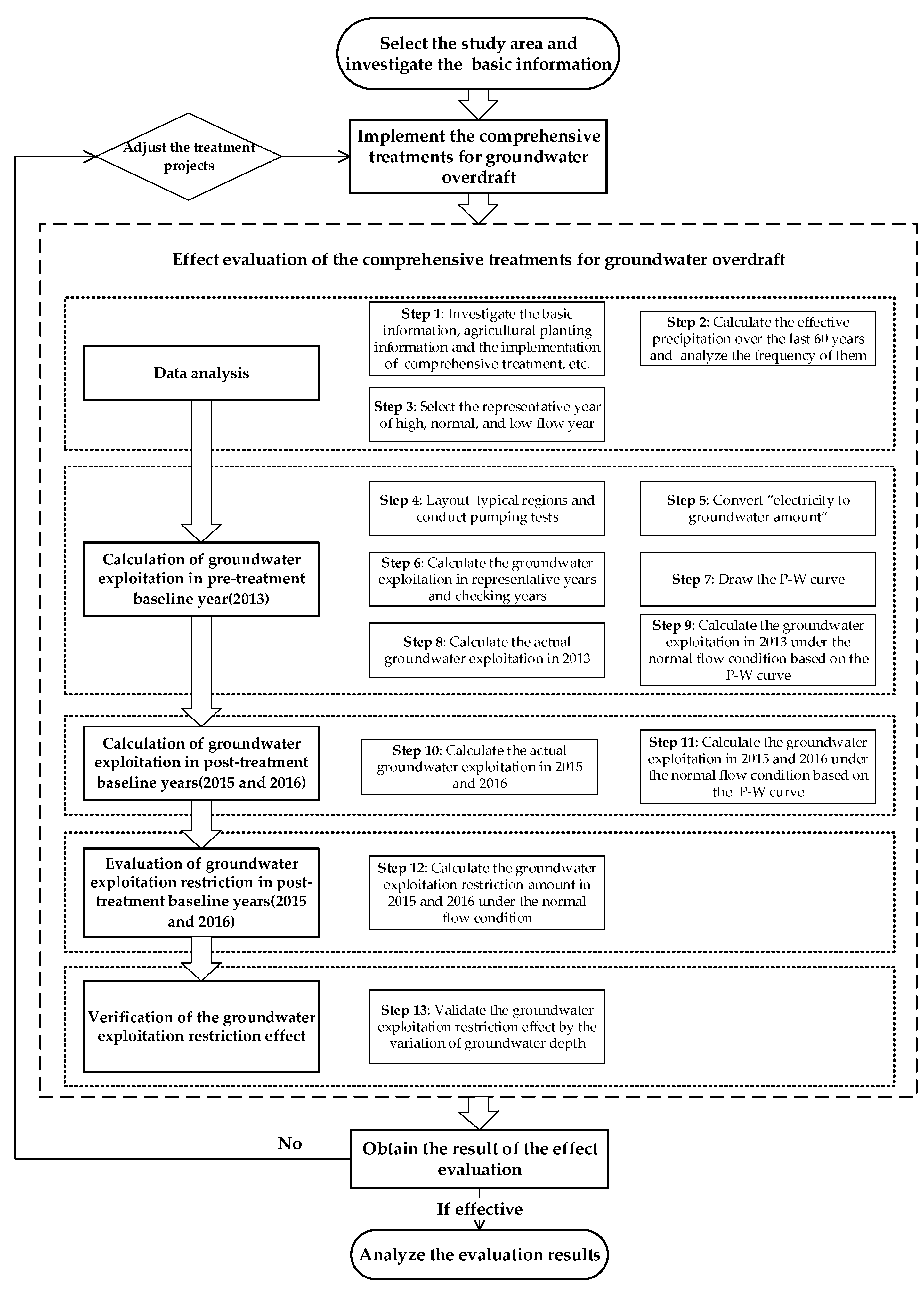
The overview of the study is illustrated by the following procedures. Considering all factors, we chose Quzhou County as the research area. After investigating all the basic information in Quzhou County, the implementation of treatment projects was carried out in the overdraft regions, which called project regions. Now, the main work of this study is to assess whether these projects have played a positive role in relieving and restoring the groundwater overdraft in the study area. The purpose of the evaluation is that, if the results of the evaluation are effective, we will affirm the treatment projects and analyze the results of the evaluation; if the results are not effective, we will make suggestions to adjust the treatment projects. The evaluation process are shown as the
Figure 2, including data analysis, calculation of groundwater exploitation in pre-treatment baseline year, calculation of groundwater exploitation in post-treatment baseline years, evaluation of groundwater exploitation restriction in post-treatment baseline years, and verification of the groundwater exploitation restriction effect by groundwater depth variation. The effect evaluation is completed by 13 steps as shown in
Figure 2.
3.2. Layout of Typical Regions and Conduct of Pumping Tests
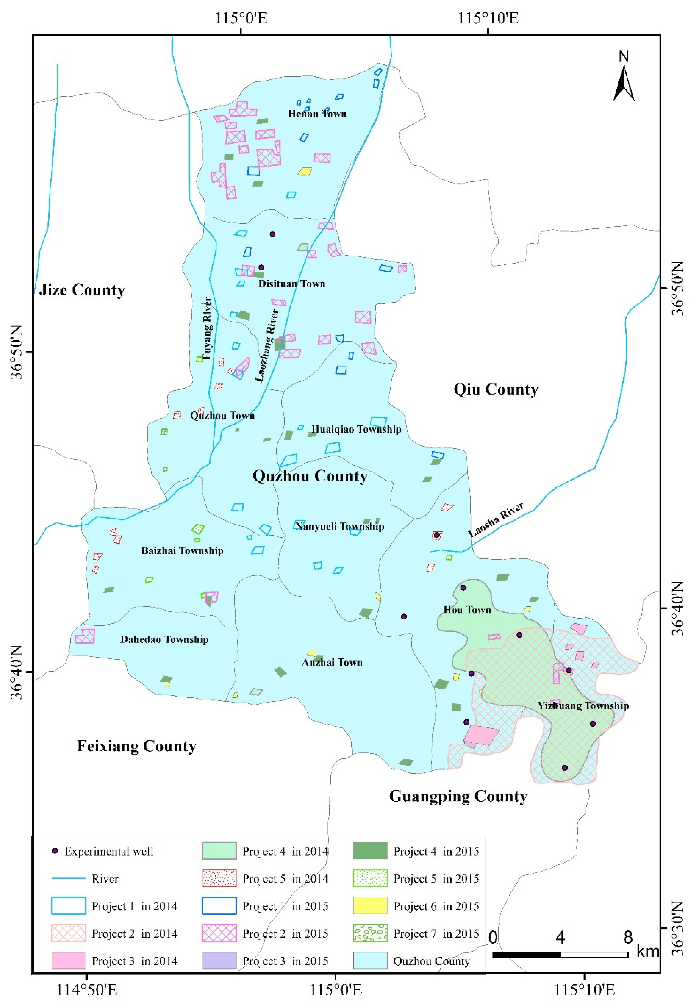
Most of the agricultural area in Quzhou County is irrigated by groundwater from wells. There are a large number of wells, supervised by individual farmers or collective organizations, scattered in the whole county. Most of the wells have not installed volume measurement facilities. However, due to the payment of electricity in the irrigation wells, the electricity consumption in the wells was generally recorded. It is the only valuable practical measurement data that can be used to calculate the groundwater exploitation amount, when combined with groundwater exploitation amount per kilowatt hour (which is called the “converting electricity to water amount”). We have selected wells both in project regions and non-project regions to conduct pumping tests and obtain the data of exploitation amount per kilowatt hour to calculate groundwater exploitation amount. According to the spatial superposition analysis of the distribution of the projects, the wells, the transformers, the soil lithology, and the crops, six typical regions were identified through the screening, which were distributed in a project 1 region, a project 2 region, a project 3 region, a project 4 region, a project 5 region, and a non-project region, respectively. Two wells in each project region and three wells in the non-project region were selected (
Figure 1).
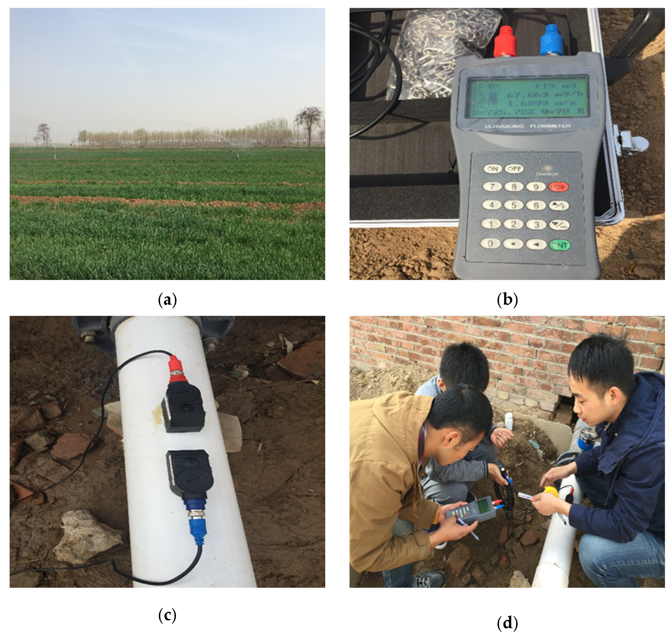
The groundwater exploitation amount per kilowatt hour in a single well is an important parameter to calculate groundwater exploitation amount. The electricity consumption was obtained by a pumping test in each observation well, and the pumping capacity was measured by a portable flow meter in the field (
Figure 3). From the tests, we obtained the groundwater exploitation amount per kilowatt hour in an individual well in the project 1 region, project 2 region, project 3 region, project 4 region, and project 5 region, which were 2.17, 1.76, 1.43, 1.28, and 1.66 m
3, respectively (
Table 2); the groundwater exploitation amount per kilowatt hour in an individual well in the non-project regions of wheat, corn, and cotton were 1.81, 1.68, and 1.52 m
3, respectively (
Table 3).
3.3. Determination of the Representative Years of High, Normal, and Low Flow
We determined the representative years of high, normal, and low flow by frequency distribution of effective precipitation. Effective precipitation refers to the amount of precipitation needed to meet crop evapotranspiration during crop growth period. Because precipitation can be stagnant in soil, the larger precipitation per day may be effectively utilized by crops in the next few days, so effective precipitation has statistical characteristics of time periods. Through fitting tests, we found that the fitting curve of effective precipitation in 10 days and agricultural groundwater exploitation in the county has the optimal structure and highest fitting degree, so the effective precipitation was counted by the 10-day scale. Effective precipitation is closely related to crop water requirement, and the study counted effective precipitation by calculating crop water requirements. The daily crop water requirement was calculated by the crop coefficient method, and the calculation formulas are as follows:
where
Pec is effective precipitation during crop growth period of a certain crop, mm;
Ptei is the effective precipitation in 10 days, mm/(10 day);
Pte is the effective precipitation in 10 days, mm/(10 day);
Pt is the precipitation in 10 days, mm/(10 day);
Wtc is crop water requirement in 10 days, mm/(10 day);
Wdc is daily crop water requirement, mm/day;
ETc is reference crop evapotranspiration, calculated by the Penman–Monteith formula, mm/day; and
Kc is the crop coefficient, determined by the method of piecewise single value average crop coefficient.
Based on the planting structure of the county and the effective precipitation during crop growth period of a certain crop, which were calculated by Equation (1), we calculated the yearly effective precipitation of the county by Equation (2):
where
Pe is effective precipitation in a year of the county, mm/year;
Peci is effective precipitation during crop growth period of crop
i, mm/year;
Ai is the irrigated area of crop
i, km
2, and it is necessary to note that the area of irrigation could not be repeated when calculating the effective precipitation of the county; in this case, the replanting area of the crop needs to be calculated separately.
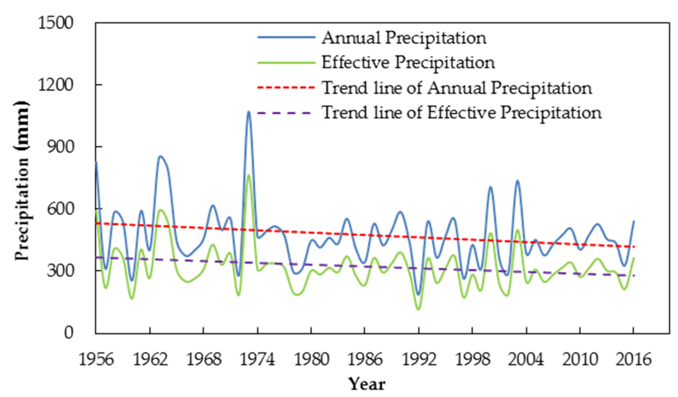
According to the temporal variations of precipitation and effective precipitation from 1956 to 2016 in Quzhou County, the inter-annual precipitation showed a significant fluctuation, and it presented a gradual decline trend with a decline rate of 18.7 mm/(10 year) on the whole (
Figure 4). Effective precipitation also presented the same change trend with a decline rate of 14.6 mm/(10 year). The multi-year average precipitation and effective precipitation were 474.5 and 321.1 mm, respectively. The minimum precipitation and effective precipitation were 187.5 and 115.7 mm, respectively, which occurred in 1992, while the maximum precipitation and effective precipitation were 1069.6 and 763.6 mm, which were 5.7 and 6.6 times the minimum value, respectively, which happened in 1973. From the above results, the annual precipitation was distributed unevenly.
In order to determine the high, normal, and low representative years, we ranked the effective precipitation from 1956 to 2013 (the precipitation series before the treatments) and applied the Pearson III curve to fit and check the series (the fitting degree was 0.95). According to the fitted curve, the reference effective precipitations with frequency of 25, 50, and 75% were 363.7, 308.5, and 249.5 mm, respectively, which were recorded as P25, P50, and P75, respectively. Based on the P25, P50, and P75, we selected the high, normal, and low representative years within a recent 10 years (from 2004 to 2013), which were 2012, 2005, and 2006, respectively. The effective precipitation of the representative years were 360.0, 308.5, and 248.2 mm, respectively, which were recorded as Pe-h, Pe-nor, and Pe-l, respectively.
3.4. Calculation of Groundwater Exploitation in the Representative Years of High, Normal, and Low Flow
Based on the results of the irrigation regions investigation and the agricultural planting structure analysis, the data obtained by pumping tests, and the agricultural irrigation electricity consumption data, we calculated the groundwater exploitation in the high, normal and low flow representative years. If there were
N groundwater irrigation regions in the county, and there were
S crop types in each irrigation region in 2013, the calculation formulas are as follows:
where
is the irrigation area of crop
j in irrigation region
i in the pre-treatment baseline year (2013), km
2;
,
, and
are the groundwater exploitation amount per square kilometer of crop
j in irrigation region
i in high, normal, and low flow representative years (2012, 2005, and 2006), respectively, based on the crop structure in 2013, m
3/km
2, which were calculated by the agricultural irrigation electricity consumption data in high, normal, and low flow representative years and the pumping test data, listed in the
Table 2 and
Table 3; and
,
, and
are the agricultural groundwater exploitation amount of the county in high, normal, and low flow representative years, respectively, m
3.
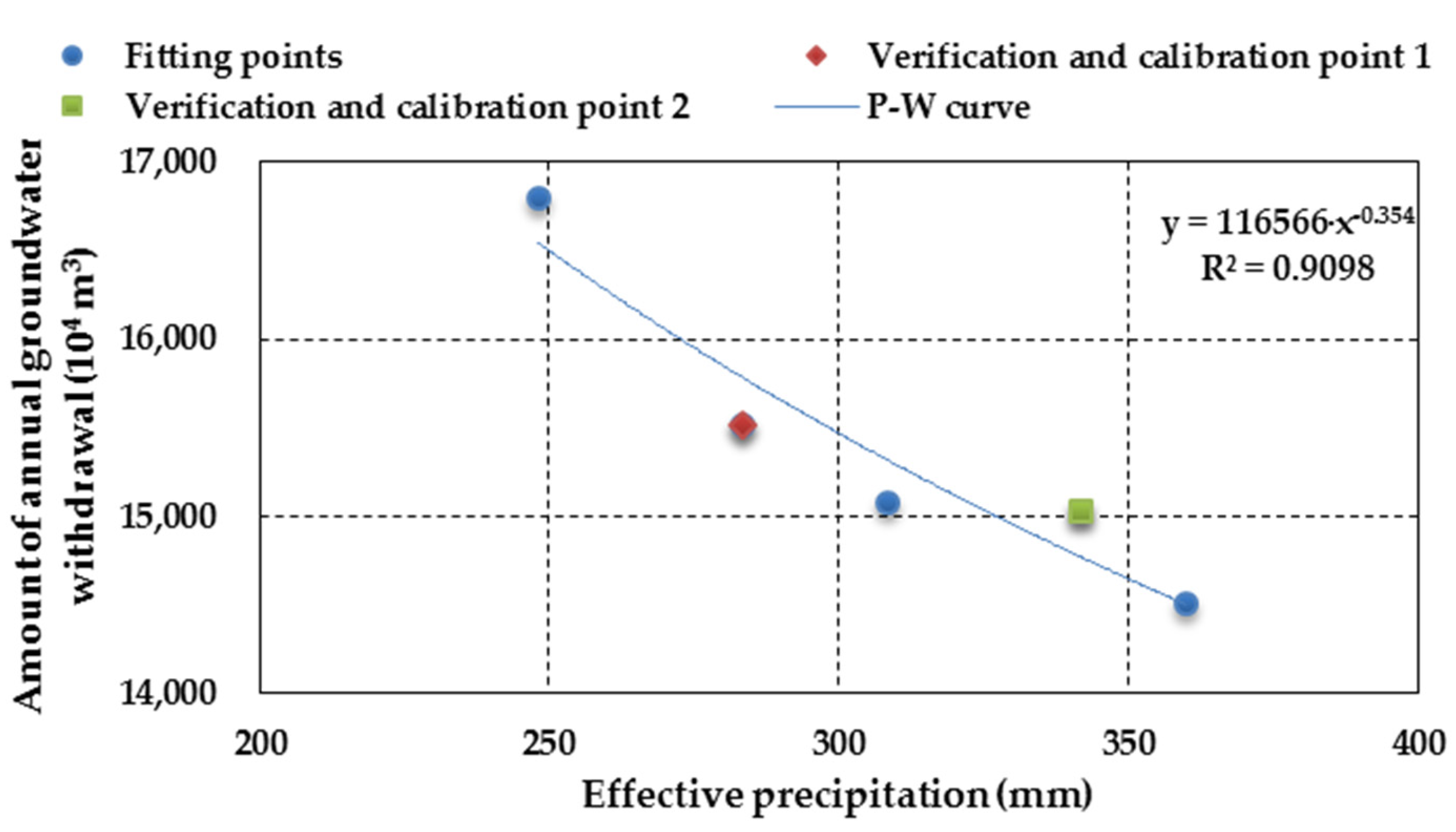
3.5. P-W Curve Drawing
The P-W curve means the relationship curve of the effective precipitation and agricultural groundwater exploitation amount. Effective precipitation is related to crop water requirement and inter-annual precipitation distribution. For specific crops, there are differences in the amount of precipitation used by crops under the same annual precipitation and different annual precipitation distribution. Crop water requirements, which have not been satisfied by effective precipitation, need to be supplemented by agricultural irrigation. As groundwater is the main source of irrigation water in this county, there is a correlation between effective precipitation and agricultural groundwater exploitation. The greater the ratio of effective precipitation to crop water demand, the smaller amount of agricultural groundwater exploitation are needed, and vice versa. By drawing the P-W curve, we can understand the change relationship between agricultural groundwater exploitation and effective precipitation more thoroughly. Based on the data we have obtained, we used the effective precipitation and agricultural groundwater exploitation amount in the representative years of high (2012), normal (2005), and low (2006) flow ((
Pe-h,
Wh), (
Pe-nor,
Wnor), (
Pe-l,
Wl)) of the county to get a power curve in the
X-Y coordinate system. Then, we chose two other years (2008 and 2013) in the recent 10 years to validate and calibrate the curve. After using the corresponding data to check the power curve, we finally obtained the optimal P-W curve (with determination coefficient
R2 = 0.9098) (
Figure 5).
3.6. Calculation of Groundwater Exploitation Restriction Amount
Because the frequency and the annual distribution of the precipitation in the pre-treatment baseline year (2013) and post-treatment baseline years (2015 and 2016) were inconsistent, it was obviously lacking a comparison basis and was thus less scientific to calculate the groundwater exploitation restriction by the difference of the actual agricultural groundwater exploitation in the pre-treatment baseline year and post-treatment baseline years. If the pre-treatment baseline year is a low flow year, while the post-treatment baseline years are high flow years, there is no need to implement any measures, and the agricultural groundwater utilization may be reduced. Conversely, the groundwater exploitation may even increase after the implementation of restriction measures. Therefore, we converted the actual agricultural groundwater exploitation of the pre-treatment baseline year and post-treatment baseline years to the condition of a normal flow year, then evaluated the agricultural groundwater exploitation restriction.
The actual amounts of agricultural groundwater exploitation in the post-treatment baseline years were calculated by Equation (4):
where
is the actual amount of groundwater exploitation in 2015 or 2016, m
3;
is the groundwater exploitation per square kilometer of crop
j in irrigation region
i in 2015 or 2016, m
3/km
2;
is the irrigation area of crop
j in the irrigation region
i in 2015 or 2016, km
2; and
N and
S are the same as mentioned above.
The agricultural groundwater exploitation under the normal flow condition in the post-treatment baseline years were obtained by a conversion coefficient. The conversion principle is that the ratios of the groundwater exploitation in different years and the groundwater exploitation under normal flow conditions in a region are relatively stable. The conversion equations are as follows:
where
is the groundwater exploitation amount under the normal flow condition in 2015 or 2016, m
3;
is the groundwater exploitation amount under the normal flow condition in 2013, m
3, which was obtained from the P-W curve corresponding to the precipitation of the frequency of 50% (
P50); and
is the groundwater exploitation amount obtained from the P-W curve corresponding to the effective precipitation in 2015 or 2016, m
3.
Based on the comparison of the agricultural groundwater exploitation amount under the condition of normal flow in pre-treatment baseline year and post-treatment baseline years, we calculated the restriction amount of agricultural groundwater exploitation in 2015 and 2016 by Equation (6):
where
is the restriction amount of agricultural groundwater exploitation in 2015 or 2016, m
3; and the other symbols are the same as those described above.
5. Conclusions
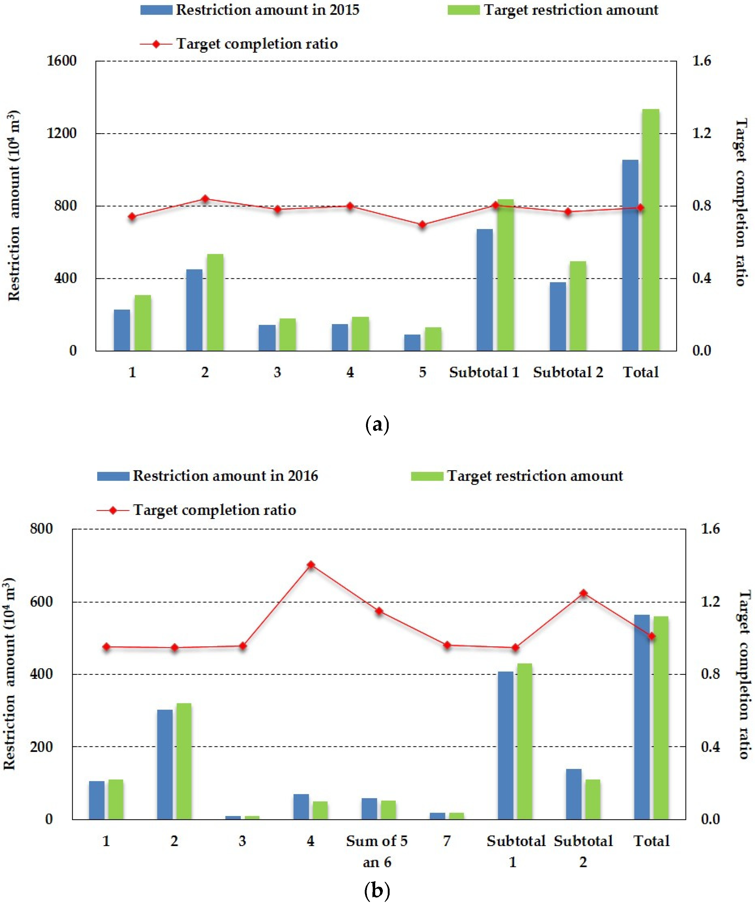
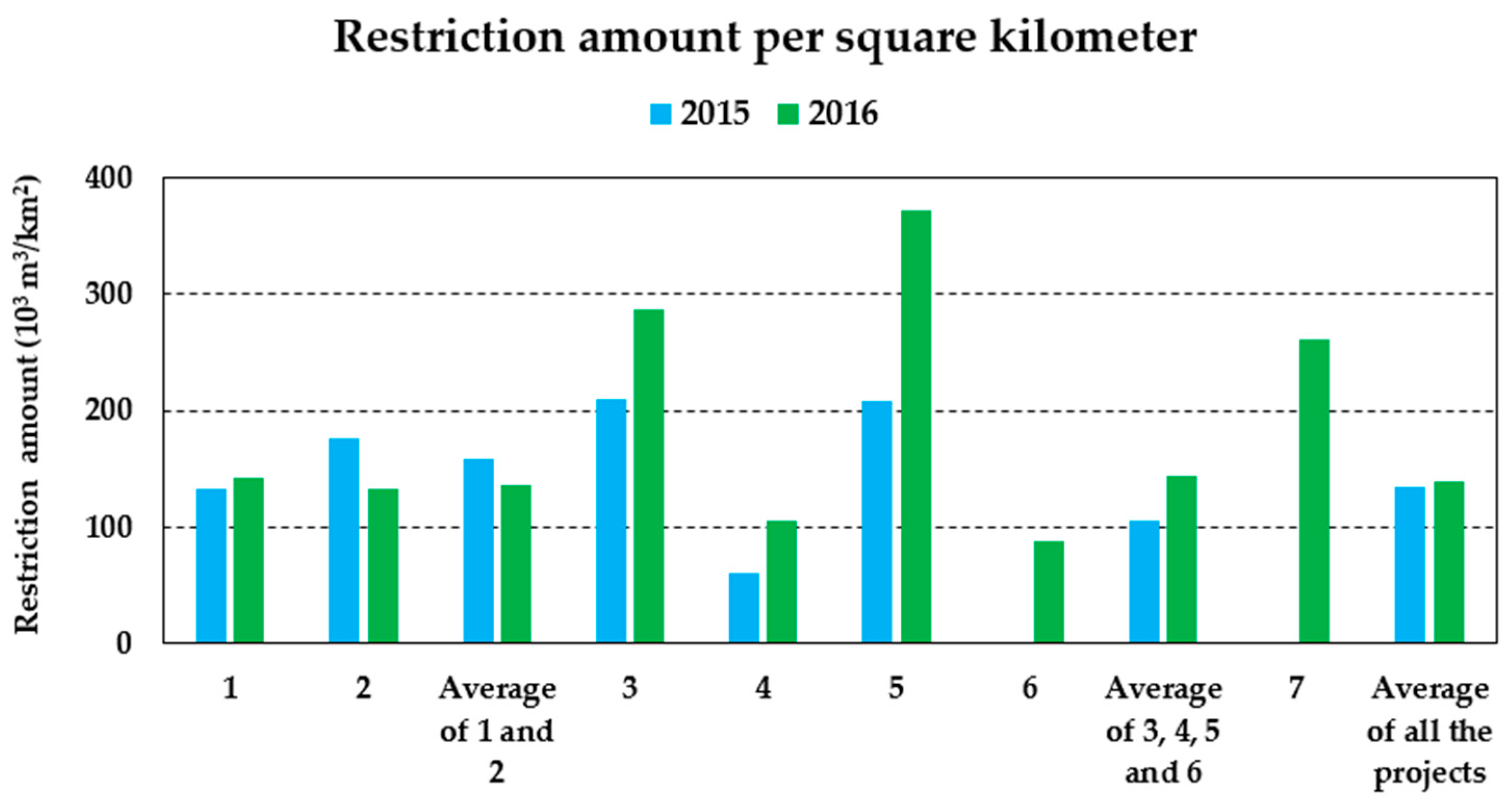
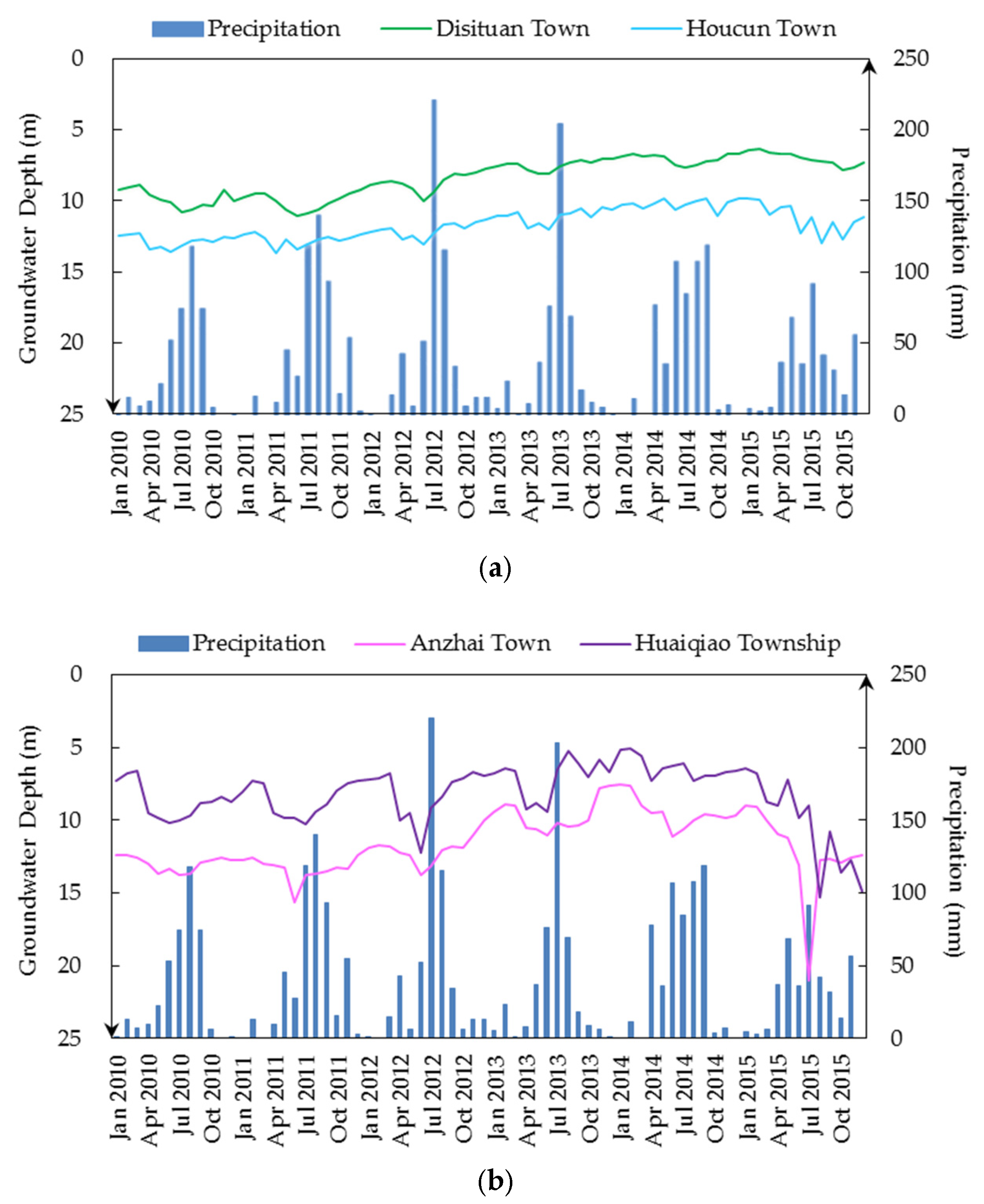
The results of field pumping test showed that the water consumption of vegetables was the largest in the test area, followed by wheat. From the view of both the target completion ratio and the restriction amount of groundwater exploitation per square kilometer, the values in 2016 were all higher than in 2015. This demonstrates the restriction effect in 2016 was better. Among different kinds of project, the completion ratios of the water and fertilizer integration of vegetables projects and the surface water substituting groundwater projects in 2015 were not high. However, both of them greatly improved in 2016, indicating that the technology of groundwater restriction is progressing continuously. The water-saving of spring irrigation for winter wheat projects has the highest completion ratio according to the results of 2015 and 2016, but the restriction amount per square kilometer were relatively low. The water and fertilizer integration of vegetables projects have the highest restriction amount per square kilometer, followed by the planting structure adjustment projects. In general, the restriction effect of the agricultural projects was better than that of the water conservancy projects. In addition, the restriction effect of the forestry projects was also obvious. Finally, the variations of groundwater depth demonstrated the restriction measures had an effective influence on the recovery of the groundwater depths. All in all, the comprehensive treatments implemented in 2014 and 2015 in Quzhou County have achieved effective results.
At the same time, the study found that precipitation has been decreasing on the whole since 1956, indicating that the exploitation amount of groundwater is bound to increase in order to ensure grain production. However, although precipitation in 2015 was greatly reduced, the exploitation of groundwater did not increase. Therefore, we conclude that, even if it is a low flow year, the amount of groundwater exploitation can be controlled by the implementation of restriction measures. In addition, based on the analysis of agricultural data, we found that the restriction of groundwater exploitation did not cause the reduction of grain production; on the contrary, there was a slight increasing trend in grain production (with an increasing rate of 5850 kg/km2 per year from 2013 to 2015). The total planting area of grain in the county was 547.9 km2 in 2013, and the production was 782.1 thousand kg per square kilometer. The total planting areas of grain in 2014 and 2015 were 564.0 and 571.7 km2, respectively; and production was 790.8 thousand and 793.8 thousand kg per square kilometer, respectively. Furthermore, the production of other economic crops has also increased, such as the increasing rates of vegetables and cotton, which were 162.0 thousand and 172.5 kg/km2 per year, respectively, from 2013 to 2015. The comprehensive treatments in the project regions have not influenced the grain yield. Therefore, comprehensive treatments can also reduce energy consumption and reduce carbon emissions, which is of great significance for the green and sustainable development of the region and the global world.
Although the restriction effect is significant, there are still many aspects that need to be further improved. In future, a comparison can be made with the research results of the water balance method. In addition, the exploitation of groundwater is mainly dependent on fossil-fuel generated electricity in the county, which may produce large amounts of carbon emissions, and solar or wind power generation can be developed in the future.

 ,
, 


