Article

A Stakeholder Oriented Modelling Framework for the Early Detection of Shortage in Water Supply Systems

1
Water Research Institute, National Research Council, Area della Ricerca di Roma 1, Strada Provinciale 35d, km 0,7, 00015 Montelibretti, Rome, Italy
2
National Civil Protection Department, via Vitorchiano 2, 00189, Rome, Italy
*
Author to whom correspondence should be addressed.
Water 2018, 10(6), 762; https://doi.org/10.3390/w10060762
Submission received: 14 May 2018 / Revised: 5 June 2018 / Accepted: 6 June 2018 / Published: 11 June 2018
(This article belongs to the Special Issue Climate-Water-Ecosystem-Interaction)

Abstract

:
Management of water supply systems under shortage conditions due to drought requires computational tools able to relate the past precipitation regime over different time scales to future water resources availability. This work proposes a modelling framework to address the occurrence of shortage for water supply systems whose resource is constituted by natural or artificial reservoirs. The proposed methodology aims at identifying “management triggers” for possible mitigation measures. Emphasis is given on the use of standardized indices to promote information sharing. The implemented tool is structured into five modules: “hydrological” module; “scenarios” module; “reservoir” module; a module for the evaluation of “indices of shortage”; and a “support to early-warning” module. The whole procedure has been applied to three Italian reservoirs. For each water body, a case specific shortage early-warning system, based on standardized precipitation indices has been identified, allowing the implementation of efficient local mitigation measures.

Graphical Abstract

1. Introduction

According to the guidelines from the European Expert Network on Water Scarcity and Droughts [1], water scarcity is defined as “a situation where insufficient water resources are available to satisfy long-term average requirements. It refers to long-term water imbalances, where the availability is low compared to the demand for water”. It can be triggered by a drought condition, defined as a natural event characterized by a significant decrease in precipitation lasting for a limited period of time (from few months to few years). Therefore, water scarcity can be determined both by natural force and by man-made actions [2]. These two strongly interconnected components can lead to shortage conditions in water supply systems (WSS), assumed as a temporary imbalance between availability of water resources and the demands associated with them.
From a climatological point of view, drought can be characterized in terms of frequency, duration, severity, and the extent of precipitation anomaly. However, with respect to other natural phenomena, impacts of drought unfold far beyond the precipitation negative anomalies and with different modes and times. For this reason, it is generally accepted (e.g., [3,4]) that there is a distinction between: meteorological, agricultural, hydrological, and socio-economic drought. Typically, these four types occur in successive steps and for different periods, possibly overlapping. Moreover, due to the complexity of drought phenomena, it is very difficult to recognize the numerous factors affecting the causal chain that propagates from meteorological to socio-economical droughts and, even more, to assess each single “weight” on the overall impact [1,5]. Such a complexity poses serious issues of characterization that makes it difficult to discover unique solutions in both adaptation and mitigation measures. One crucial aspect in the assessment of drought mitigation measures, as pointed out in the Drought Management Plan Report [1], is to establish an appropriate link between a basin drought state and possible management actions [6,7]. As stated by Gustard et al. [8] “the basis of any drought management plan is a robust system of indicators that can identify and diagnose anomalies in water availability and can provide the basis for early detection of drought episodes”. In this context, drought monitoring and early warning indicators are fundamental components of a drought risk management approach [9,10,11,12], which enable a system of analysis to detect the unique characteristics of drought in terms of both precipitation anomalies and conditions of shortage. Such an analysis should lead to the identification of “triggers” for the implementation of specific mitigation measures, recognized among stakeholders [13,14]. However, as the interdependence of all users increases due to the ramified network of direct and indirect drought impacts [15], management of water systems can be very difficult due to the potential conflict of interests among users, affecting the social acceptance of drought management measures [16,17,18]. In this context, it is crucial that “triggers” based on specific indicators are objectively defined and able to clarify the relation between drought severity (in meteorological terms) and possible impacts [19,20,21]. This relationship must be assessed considering that impacts can be very different and can be deployed on very different time scales depending on the different users. For this reason, some authors have proposed drought indices based on the combination of several meteorological and/or hydrological variables in a multivariate analysis framework [22,23]. In order to be useful to support drought management, indicators should be capable to meet the actual information needs of the different decision-makers [24]. Moreover, one has to consider indicators defined at the basin scale, in order to take into account the WSS as a whole, including natural and human factors [25,26,27,28]. Finally, indicators should take into account the related uncertainty. It is worth noting that according to Zare et al. [29], the keyword “uncertainty” is the least mentioned in the field of Integrated Water Assessment and Modelling (IWAM), despite its fundamental importance (conversely, the keyword “management” is the most cited).
It must be stressed that issues related to quantitative water management in drought and scarcity conditions can be strongly related to quality problems, due to possible increased concentrations of contaminants. This aspect is explicitly mentioned, for example, in the Guidelines for drinking-water quality of the World Health Organization [30]: Water Safety Plans should include a risk analysis of possible shortages to estimate the risk of not reaching quantity and quality targets. Scarcity is only one of the possible hazards that define risk for WSSs. In this paper, other factors such as infrastructure vulnerability, exposure to contamination, loss costs (e.g., [31,32,33,34]), are not taken into account.
To cope with drought and scarcity from a management perspective, it is possible to adopt support tools, such as AQUATOOL [35], MODSIM [36,37,38], WEAP [39], RIBASIM [40], WARGI-SIM [41] or SimBaT-DSS [42], or a set of interacting models such as the Netherland Hydrological Instrument NHI [43], which basically computes the transient water budget of integrated WSSs. A comparison of generic simulation models for water resource systems can be found in [44]. However, these kinds of tools do not adopt or partially adopt indicators to characterize drought, scarcity and related impacts and the links among them, as required in the framework of the Drought Management Plan [1].
To quantitatively address drought characterization, in this paper we propose a stakeholder oriented modelling framework for the early shortage detection when the water resource is constituted by a reservoir fed by surface waters. Our focus is placed on the quantitative characterization of water shortage events and we aim to provide a robust and sharable basis for water basin policies, intended as a catalogue of management actions based on the allocation of water under scarcity conditions. In this regard, the use of standardized indices to characterize both meteo-hydrological drought and shortage conditions is extensively exploited, according to the EU standards [1]. From this perspective, the proposed methodology constitutes a novelty with respect to the numerical codes mentioned above. The developed procedure has been implemented in a single code, named INOPIA, experimented by the National Civil Protection Department as a pre-operative analysis tool. In order to explore the potentialities and limits of the whole procedure, three case studies having different features such as precipitation regime, climate, catchment size and reservoir capacity, seasonal demand, etc., are analyzed: Lake Maggiore (Switzerland and Northern Italy), the Ridracoli reservoir (Central Italy), and the Occhito reservoir (Southern Italy).

2. Materials and Methods

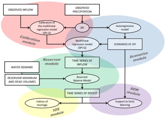
2.1. Methodological Framework

The methodological procedure proposed in this paper results from a deep consultation with the National Civil Protection Department, as a principal stakeholder, and with the water managers of several reservoirs, as final users. The initial consultation aimed at defining the decision-makers’ information needs. Some guidelines have been agreed upon, beginning with the results of the stakeholders’ consultation, that aim to obtain an operational system according to the European standards [1] and, at the same time, to pursue the goal of “facilitation and transparency” as a pillar for stakeholders’ involvement [14]. In the following, the main outcomes of this consultation are reported:
  • Variables of interest and results, for climate, hydrological and water management analysis should be expressed in terms of normalized indices, easily understandable by stakeholders and policy-makers to allow for comparisons among different the basins and WSSs or sub-systems. Among them, the Standardized Precipitation Index (SPI, [45]) to characterize the meteorological drought is preferred [46,47].
  • The whole procedure must relate directly to meteorological drought indices and severity indices (i.e., ability to meet demands) as impact metrics.
  • Simple basin scale rainfall-discharge models are necessary where a climate monitoring network is poor, especially in the upper part of a river basin, provided that such models are able to reproduce the dynamic of the system due to climate variability. Model simplicity (both in operative handling and in calibration procedures) enables the implementation and comprehension of the hydrological tools required for non-expert users. This is a key point in a participatory management framework [14].
  • The precipitation and hydrological time series used to estimate water resource availability must be representative of the characteristic return periods of shortage events. For this reason, a stochastic approach should be preferred.
Taking into account the agreed upon guidelines, the following specific tools have been developed:
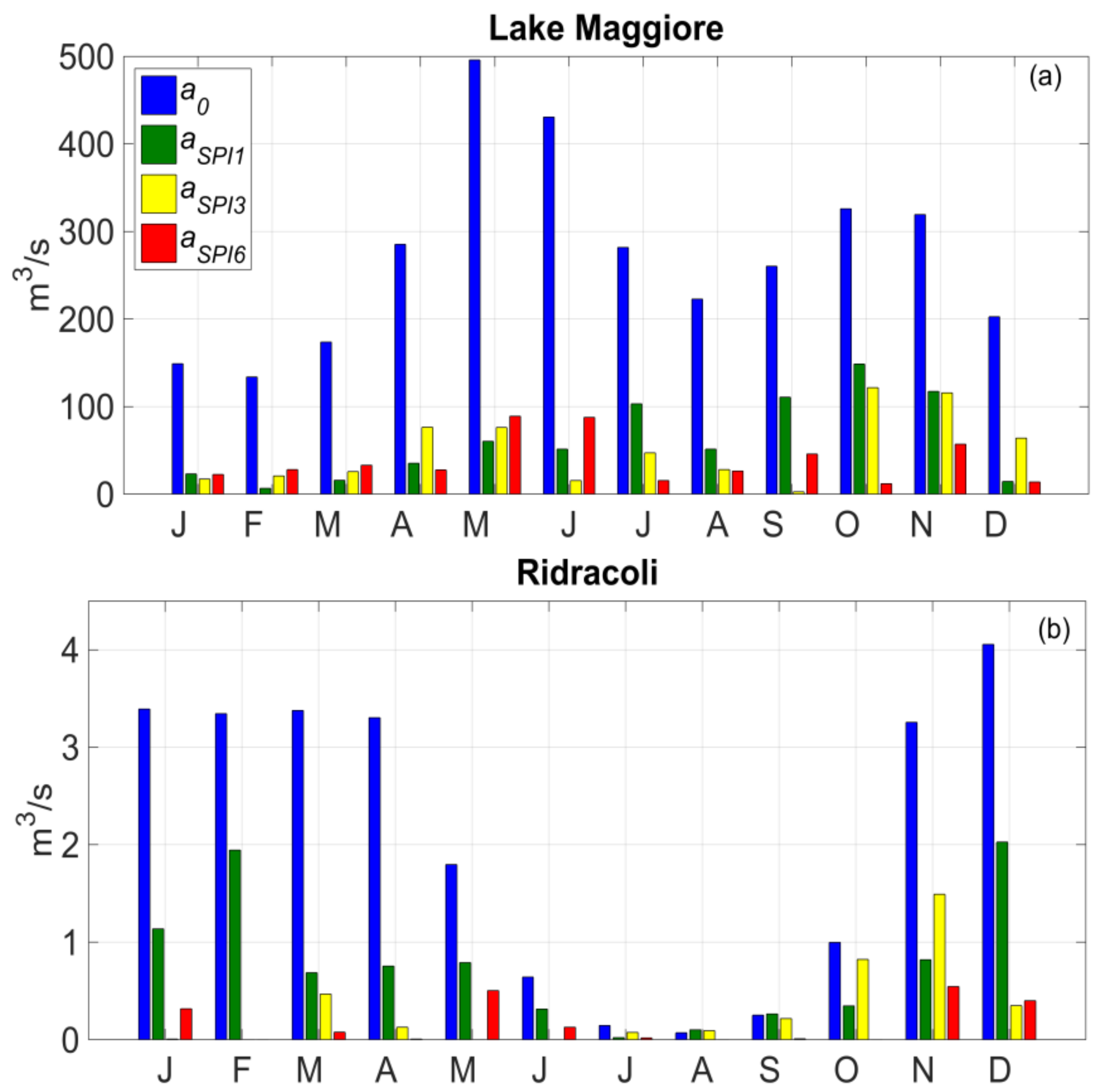
  • A multilinear regression model, named SPI-Q, to simulate the relationships between the precipitation regime, represented by SPIs computed over different time scales and the monthly inflow to the reservoir (Section 2.1.1).
  • A stochastic model for the monthly SPI based on a zero-mean autoregressive (AR) model to generate a long-enough time series (Section 2.1.2).
  • A monthly water balance model of the reservoir that accounts for the storage of the reservoir, the inflows and outflows connected to the water demands, environmental flows, and flood control spillages (Section 2.1.3).
  • Suitable indices of shortage able to represent not only the mean failure conditions, but also the “extreme” failures (i.e., with longer return periods), less likely, but potentially more dangerous (Section 2.1.4).
  • Statistical methods for a quantitative analysis of the past precipitation regime, represented by the SPIs and the future conditions of shortage, assessed over different forecast time scales (Section 2.1.5).
The overall five-modules framework is presented in Figure 1, where each module is indicated by ellipses: (1) Calibration, (2) Scenarios, (3) Reservoir, (4) Indices of shortage, (5) Support to early-warning.

2.1.1. CALIBRATION Module

The relation between precipitation and inflow to the reservoir is simulated by a multilinear regression model called SPI-Q model [48,49,50,51], computed at the monthly scale:
Q ( m , i ) = a S P I 1 ( m ) · S P I 1 ( m , i ) + a S P I 3 ( m ) · S P I 3 ( m , i ) + a S P I 6 ( m ) · S P I 6 ( m , i ) + a 0 ( m )
where Q ( m , i ) is the inflow to the reservoir for the month m, year i, and S P I 1 ( m , i ) , S P I 3 ( m , i ) , and S P I 6 ( m , i ) are the means over all the available stations of the Standardized Precipitation Indices [45] computed for the month m, year i on the precipitations cumulated over 1, 3, and 6 months. To compute the SPI values, a gamma distribution has been adopted [52,53]. As such, the data requirement for SPI-Q model application is limited to the monthly time series of precipitation, representative of the analyzed watershed basin and contemporary monthly inflows to the reservoir.
a S P I 1 ( m ) , a S P I 3 ( m ) , a S P I 6 ( m ) and a 0 ( m ) are the coefficients from the multilinear regression of SPI1, SPI3, SPI6 and the known term, respectively. These coefficients are calibrated for each month m adopting the least-square method.
It is worth noting that the regression coefficients (having the units of a discharge) can be interpreted in a physical perspective, as they express the relative weights that hydrological processes developing over different time scales have on the monthly discharge. a 0 ( m ) represents the mean discharge under mean conditions of precipitation, as the latter correspond to null values of SPI1, SPI3, and SPI6; a S P I 1 ( m ) , a S P I 3 ( m ) , a S P I 6 ( m ) represent the weights that the precipitation anomalies over a certain time scale have on the discharge (inflow to the reservoir). Moreover, the ratio between each coefficient and the known term a 0 ( m ) can be regarded as the impact that cumulated precipitation has on the discharge anomalies. Low values of the coefficients with respect to a 0 ( m ) indicate a stability of the discharge regime with respect to the precipitation anomalies, whereas high values indicate that discharge variability is explained by precipitation cumulated over a given time scale.
The choice of the aggregation time scale (1, 3, and 6 months) and the related physical meaning of the regression coefficients reflect the typical time scales of the different hydrological processes that can contribute to the total inflow to the reservoir: SPI1 is representative of the processes with fast response time (i.e., surface run-off). SPI3 can be considered representative of the mean actual conditions of soil moisture, which in general are influenced by the precipitation aggregated over a time series longer than one month. Moreover, this time aggregation is recognized as the most representative for agricultural drought, thus having a strong correlation with the vegetation response [54,55,56]. Finally, SPI6 represents slow hydrologic processes, such as snow melting and subsurface flow. Such aspects will be discussed in details in Section 3.1.

2.1.2. SCENARIOS Module

Once calibrated, the SPI-Q model is adopted to design different scenarios of inflow to the reservoir from assigned precipitation time series through the SCENARIOS module. The basic assumption is that the response of the catchment to the precipitation regime is time-invariant. Such a hypothesis is assumed adopting the constant values of the regression coefficients in Equation (1) to generate scenarios of inflow from precipitation scenarios. From a physical perspective, this means that the land use of the watershed basin as well as the infrastructure (i.e., possible connections to external basins or caption works) remain unchanged in time and independent from the precipitation regime.
In this paper, a synthetic time series of monthly precipitation has been used to generate a discharge time series. Adopting a synthetic time series of precipitation and/or discharge to simulate the impacts of drought events on WSSs is a widely acknowledged method, as it allows for combining several conditions of precipitation (or discharge) to the actual storage in the reservoir [57,58,59,60,61]. Here, we preferred to generate a precipitation time series with respect to discharge, as usually historical records of precipitation are longer than discharge records, which allowed us to compute more robust statistics. The generation method adopted in this research is based on a zero-mean autoregressive (AR) model [50] that allows generating SPI1 time series statistically equivalent to the observed ones, thus reproducing the natural variability along a wide range of time scales. Synthetic SPI1 time series are transformed into monthly precipitation by inverting the cumulated density functions fitted in the CALIBRATION module to compute the SPI1 and finally turned out into monthly inflow time series through the SPI-Q model. It is worth it to stress that the inflow scenarios can be developed from both time series of precipitation (i.e., from medium term weather forecast) or directly from Standardized Precipitation Indices time series. The latter approach can be particularly useful when implementing climate change scenarios from General Circulation Models (GCMs) output. In fact, as the SPI is normalized (by construction), no statistical downscaling is required when implementing precipitation scenarios from GCM.

2.1.3. RESERVOIR Module

In this module, the water balance of the reservoir is computed at a monthly scale considering as budget terms the inflow from the SPI-Q model and the monthly water demand addressed to the reservoir (including possible environmental flow). The quantitative status of the reservoir is computed as stored volume, taking into account maximum and dead capacities. Conditions of failure occur when the stored volume reaches the dead capacity; accordingly, the water demand not satisfied is considered as a water deficit. Conversely, overflow conditions occur when the monthly inflow exceeds the maximum reservoir capacity.

2.1.4. Indices of Shortage (IOS) Module

This analysis allows for the statistical quantification of the exposure of the water system to failures by estimating the probability of occurrence, duration, and intensity of the water deficit (Reliability-Resilience-Vulnerability metrics) based on the output from the RESERVOIR module. A classical approach based on the Reliability, Resilience, and Vulnerability (R-R-V) metrics (e.g., [62,63]) has been adopted, although slightly modified to also take into account extreme events [49]. Such kind of metrics have been recognized as the most important objectives for water utilities and for stakeholders in general [64].
Reliability is defined as the probability of the system to perform in a satisfactory way during a defined operation period [65]:
R e l = n s T
where ns is the number of satisfactory time steps (i.e., a time step during which the demand is fully satisfied) and T is the number of time steps in the whole operation period, thus 0 R e l 1 (dimensionless), assuming monthly time resolution throughout the analysis [66].
With regard to the water reservoir, resilience is commonly associated to the ability of the water system to recover from adverse events such as prolonged droughts. Two indices, Resmed and Resext, are adopted to quantify Resilience. These are computed on the data set of the simulated storage failure durations in the operation period T, considering the median (perc50) and extreme (perc90) duration of the failures, normalized by the number of months per year (12):
R e s m e d = 1 1 12 p e r c 50 { m f ( i ) } i = 1 , , N f ; R e s e x t = 1 1 12 p e r c 90 { m f ( i ) } i = 1 , , N f
where Nf is the total number of failures during the operation period, mf(i) is the duration of the i-th failure, perc50 and perc90 are the 50th and 90th percentile (positive tail) of the frequency distribution of the failure durations. Splitting the Resilience metric into the median and 90th percentile also allows for the consideration of events with a long return period, as suggested in the Drought Management Plan Report from the EU Commission [1].
Similarly to reliability, two indices are adopted to measure vulnerability: median vulnerability Vulmed and extreme vulnerability Vulext:
V u l m e d = p e r c 50 { j = 1 m f ( i ) W D j ( i ) j = 1 m f ( i ) W d j ( i ) } i = 1 , , N f V u l e x t = p e r c 90 { j = 1 m f ( i ) W D j ( i ) j = 1 m f ( i ) W d j ( i ) } i = 1 , , N f
where Nf is the total number of failures during the operation period, W D j ( i ) is the deficit in the month j of the failure i and W d j ( i ) is the corresponding water demand of month j(i).
It is worth noting that the proposed metric for Reliability is based on the number of computed failure episodes with respect to the whole operation period. Similarly, Resilience and Vulnerability metrics are based on the “experimental” cumulative density functions (i.e., on the cumulative density function of duration and deficit for Res and Vul, respectively). Therefore, no theoretical distribution is assumed in advance. Such an approach is justified by using a stochastic approach to estimate the indices of shortage (Section 2.1.2). Possible uncertainties on the computed shortage indices related to the modelling uncertainty are analyzed in Section 3.4.

2.1.5. Support to Early-Warning (SEW) Module
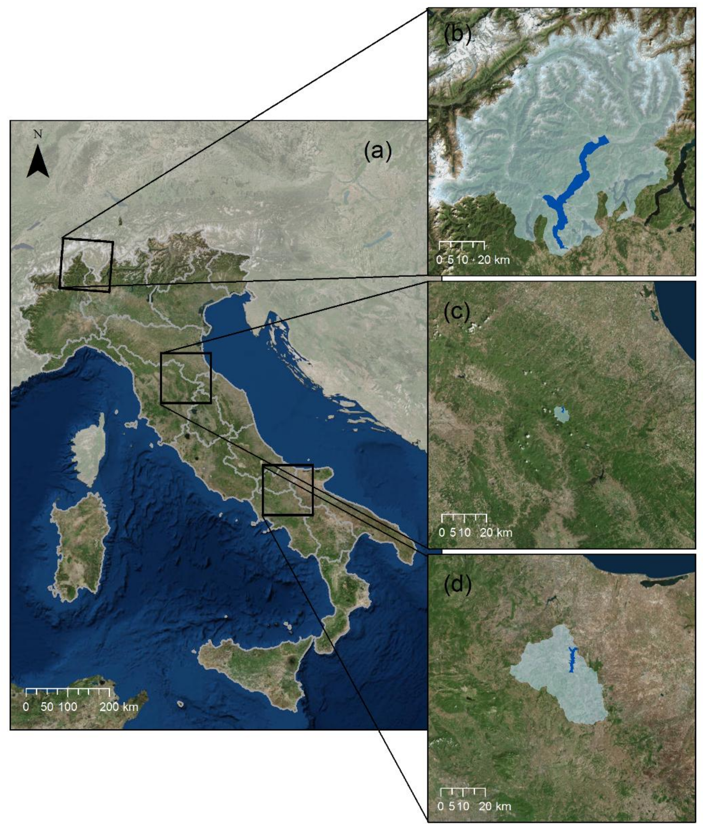
This module aims at giving quantitative information to answer the following question: giving the precipitation of the last n months, what is the probability of occurrence of deficit during the following M months? It is worth it to stress the importance of defining a specified time window of analysis in order to assess the capability of failure forecast for a given reservoir [59]. To this goal, the SEW analysis graphically links the precipitation regime, represented by the SPI computed at different time scales, to the deficit volumes computed over the M following months. Once chosen the month of analysis, the SPI time scale, and the forecast window (in the example of Figure 2 March, SPI5 and 6 months, respectively), the occurrence of failure (Figure 2a) and the correspondent cumulated deficit (Figure 2b) are plotted for different classes of antecedent precipitation anomalies, represented by the SPI at a given time scale. Similarly to Figure 2b, Figure 2c relates the actual volume in the month of analysis to the cumulative deficit occurred in the following m months (6 in the example). It must be stressed that that usually the actual water stored in a reservoir is adopted to forecast future conditions of shortage over a given time window [6,41]. However, linking the SPI to future possible failures, as in panel (b), provides the possibility to associate the probability features of the precipitation regime to the probability of occurrence and the intensity of shortage.
In addition to the analysis presented in Figure 2, where the month of analysis, the antecedent SPI time scale and the forecast window are assigned, an overview of all the combinations of SPIs with a failure forecast time window for a given month of analysis is also analyzed. Such a visualization, discussed in details in Section 3.5, allows for a quantitative assessment of the relationships aiming to find out the best predictor in terms of antecedent precipitation (SPI) and for which forecast time scale. Such an analysis permits the getting information on both possible thresholds to trigger mitigation measures and on possible management actions in case of forecasted shortage episodes. To this goal, for each SPI and deficit aggregation scale, the following procedure has been adopted.
A linear regression (red lines in the example of Figure 3) is equipped to the subset of failure events associated to a negative SPI. If the intersection of the resulting regression line with the x-axis (SPI values) is lower than zero (Figure 3b), the value of the intersection is assumed as the management threshold SPImt (mitigation measures trigger); otherwise, the linear regression is forced to pass through the axes-origin (i.e., the management threshold cannot correspond to a positive SPI, as it would imply the occurrence of the reservoir deficit even when the precipitation index is above average).
All pairs having a positive deficit associated with a SPI lower or equal to the estimated management threshold are considered as “true positives”. Events having a null deficit and associated SPI lower or equal to the estimated management threshold are considered as “false positive”. Similarly, all events having a positive (null) deficit associated with an SPI higher than the estimated management threshold are considered as “true (false) negatives”. This classifier matrix is analyzed through the Cohen’s k coefficient, a scalar metric for accuracy that compensates for success due to mere chance [67]. The strong relationship between the Cohen’s k and the Receiver Operating Characteristic (ROC) curves has been demonstrated as a tool to measure classifiers’ accuracy in binary-class problems [68], widely adopted in a water management framework (e.g., [69,70]). In the proposed procedure, the Cohen’s k has been preferred with respect to the ROC curve as the interpretation of the latter could be quite difficult, mainly in multi-class problems. The Cohen’s k coefficient is defined as follows:
k = T P F P   P ¯ · ( 1 2 N ) P P ¯ · ( 1 2 N )
where P, TP, and FP are the total number of failure events, the number of true positives, and the number of false positives, respectively. P ¯ = T P + F P and N = F P + T N (where TN is the true negative). The higher the Cohen’s k, the better the performance of the forecast. It is possible to find out the best predictor in terms of antecedent precipitation (SPI) and time scale of the forecast. Cohen’s k ranges from 0 to 1. If Cohen’s k > 0.4, the concordance is defined as fair to good [71].
The goodness-of-fit for the predictor (linear regression) is quantified through the correlation coefficient (r) computed on the associated subset. This descriptor assesses the performances of the SEW application (i.e., its capacity to quantify the expected deficit). The correlation coefficient r has been preferred to the root mean squared error or mean absolute error, as it is easier to compare among the aggregation scales and the different case studies.

2.2. Case Studies

The methodology described in the previous sections has been applied and tested on three Italian reservoirs: Lake Maggiore (Switzerland and Northern Italy), Ridracoli (Central Italy), and Occhito (Southern Italy) reservoirs. The locations of the three reservoirs are shown in Figure 4, while the main characteristics of each case-study are reported in Table 1. Mean monthly precipitation of one representative station located within the watershed basin and related inflow to the reservoir are shown in Figure 5 to describe the mean hydrologic regimes.
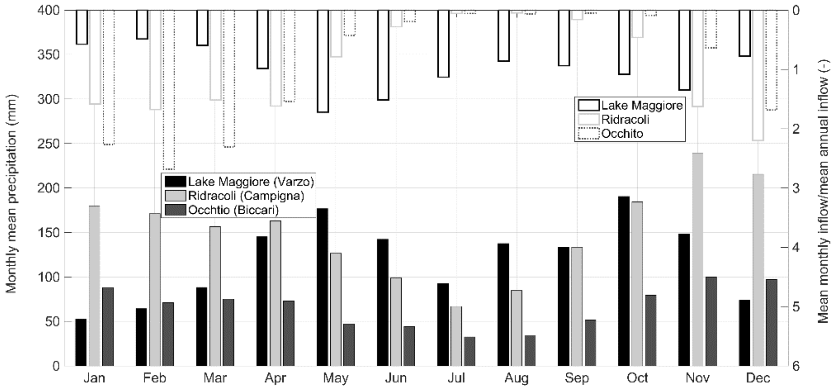
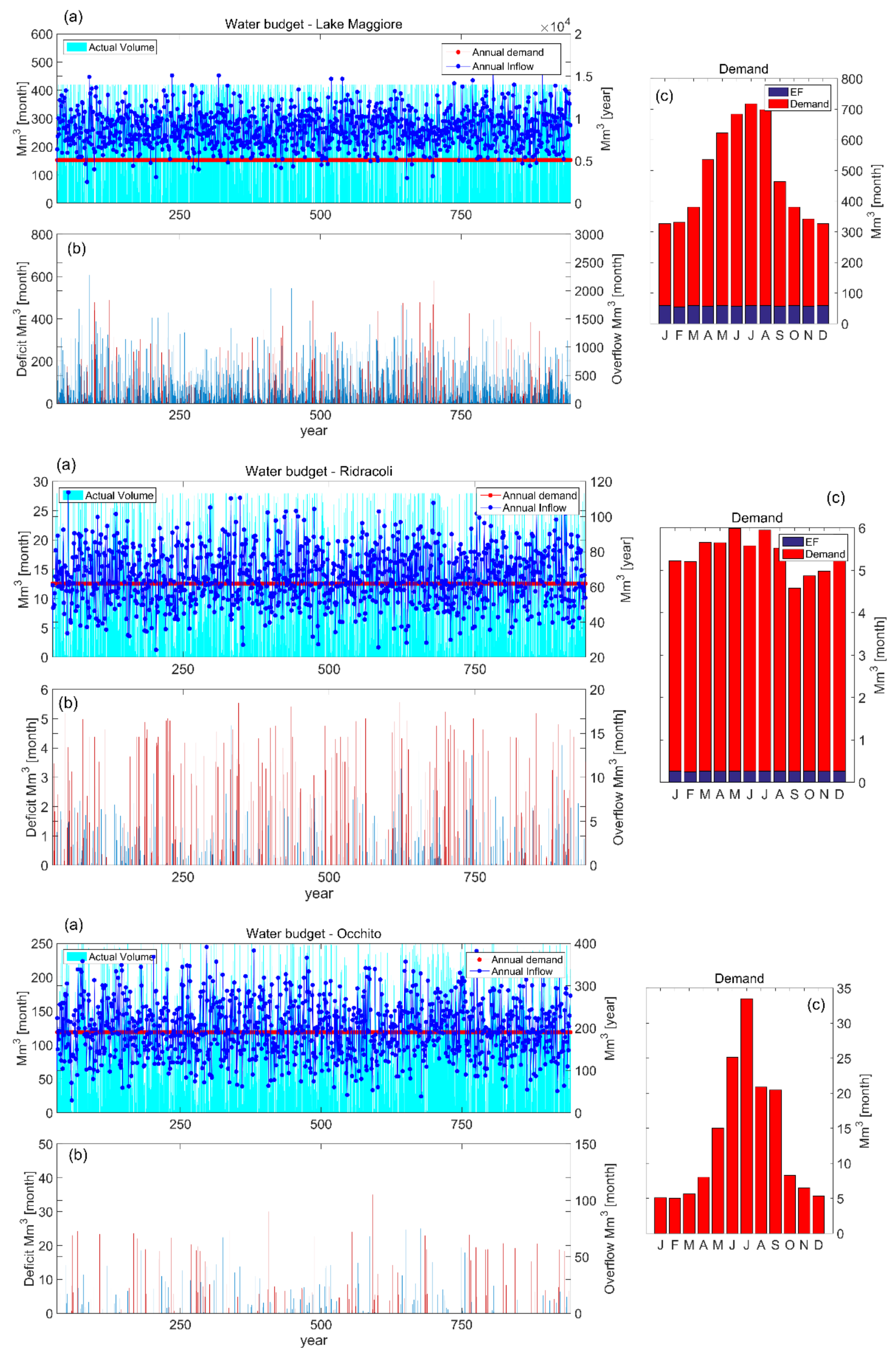
  • Lake Maggiore natural reservoir is located in the Alpine region between Switzerland and Italy. Its level is regulated by law through hydraulic infrastructures that make the total amount of water usable for irrigation and industrial purposes equal to 420 mm3 from March to October and to 315 Mm3 from November to February. The total demand ranges from approximately 250 Mm3/month in winter to 650 Mm3/month in summer (irrigation season). The monthly precipitation regime presents two peaks: the spring’s peak is due to both rainfall and snowmelt, while the autumn’s peak appears to be related only to precipitation. Moreover, the base-flow ensures a consistent discharge also during the summer months.
  • Ridracoli artificial reservoir. Located in the Tosco-Emilian Apennine chain (central Italy), it can be considered a small size reservoir (28 Mm3). The mean monthly demand (only for human consumption) is about 5 Mm3/month. The strong increase due to the touristic season is usually supplied by other water resources (in particular, coastal aquifers). In this basin, most of the precipitation occurs in late autumn, winter, and early spring. The inflow to the reservoir shares approximately the same regime and almost nullifies during the summer months.
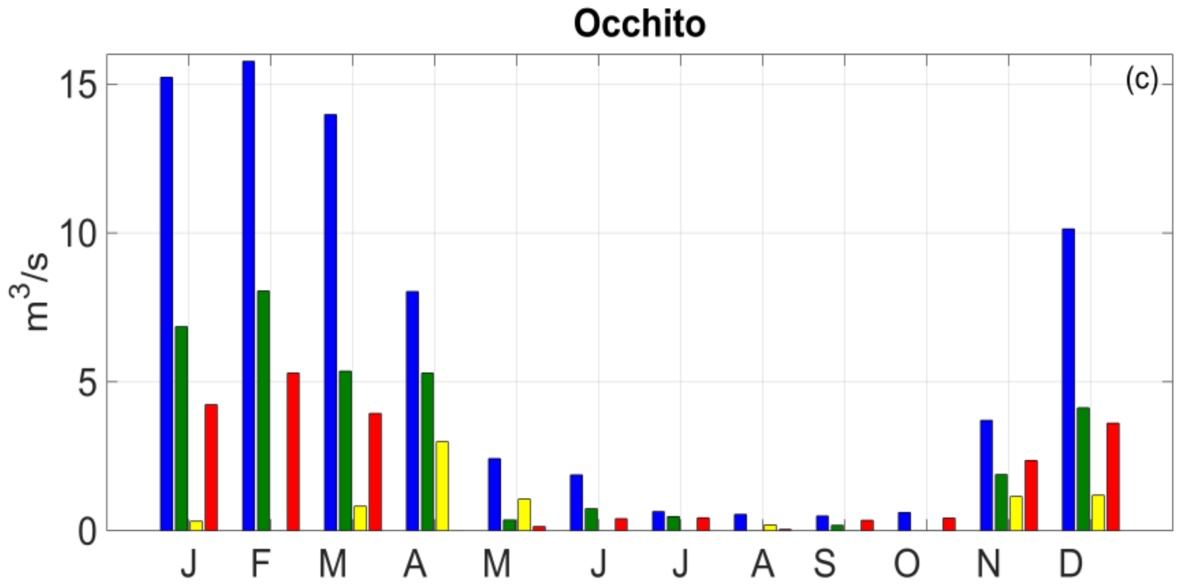
  • Occhito artificial reservoir, located in the Molise region (south of Italy) can be considered a big-size reservoir, with a maximum storage capacity of 250 Mm3. The mean annual withdrawal from the Occhito dam for the irrigation supply of the Fortore irrigation district is about 95.9 Mm3 (varying seasonally), while the annual demand for human and industrial consumption are respectively about 55 and 10 Mm3 [49,51]. The precipitation regime is similar to the one observed in Ridracoli, with most of the rainfall concentrated in late autumn, winter, and early spring. Such a precipitation regime appears to drive the inflow to the reservoir regime.

3. Results and Discussion

3.1. Calibration

To evaluate the results of the CALIBRATION module, the regression coefficients (Equation (1)) for the three case studies are shown in Figure 6. The goodness-of-fit metrics are presented in Table 2.
The performance indices (Table 2) show a good agreement between observation and simulation. Romano et al. [50] demonstrated that the modelling errors do not significantly affect the value of the shortage risk indices computed from the observed inflow time series; therefore, the SPI-Q model results can be acceptable for assessing the exposure to shortage of WSSs. It is worth noting that the mean bias, computed on an annual basis, is in the worst case (Lake Maggiore), below 10%, with respect to the reservoir capacity, and below 5% with respect to the total annual mean inflow (Occhito). The modelling error is higher for higher values of inflow, which usually does not propagate into large volume errors for small-size reservoirs, as the maximum capacity acts as a cut-off in case of overflow (i.e., for Lake Maggiore and Ridracoli reservoir, having a total annual inflow significantly higher than the maximum storage capacity). On the contrary, the modelling error can propagate throughout the simulation variables in case of reservoirs with a higher ratio between the maximum capacity and mean annual inflow. Uncertainties on the indices of the shortage related to the uncertainty on the SPI-Q model will be discussed in Section 3.4.
As shown by the mean monthly inflow (Figure 5) and by a 0 coefficients (Figure 6) the three basins are characterized by different hydrological regimes: the maximum discharge at Ridracoli and Occhito occurs in winter, whereas in summer the discharge is negligible. This is partially due to the precipitation regime (rainfall is at a minimum in July, Figure 4) and partially to the highest summer evapotranspiration, which limits run-off. On the contrary, a discharge regime for Lake Maggiore presents two peaks, during spring and autumn, related to the maximum precipitation combined with the snowmelt.
A qualitative inspection of the regression coefficients, suggests that the time variability of the discharge for a given month at Ridracoli and Occhito is driven by the precipitation of the same month (SPI1), which can be related to fast hydrological processes: in fact the a S P I 1 monthly coefficients are in both basins higher than a S P I 3 and a S P I 6 . However, during the late-autumn and winter months both at Ridracoli and Occhito, longer time scales significantly impact the discharge variability: in particular, the weights of SPI3 in autumn and the weights of SPI6 in winter are significant at Ridracoli and Occhito, respectively. Such differences in the residence time is due to the difference in size between the two watershed basins, being climate and land cover similar.
Results for Lake Maggiore look different as a S P I 3 and a S P I 6 are higher than a S P I 1 , meaning that the variability of the inflow to the lake during the spring’s months is driven by seasonal precipitation aggregated over 3 and 6 months. Such a result can be interpreted as the effect of the snow melting processes, since the inter-annual variability of discharge during the spring months is significantly driven by winter precipitation, represented by the SPI3 and SPI6 computed in May, June, and July. Conversely, in autumn (particularly in October and November) the weight of the SPI3 on the discharge variability is significant compared to that of SPI6. These findings can have a double explanation: on the one hand, summer precipitation does not impact the discharge due to the strong evapotranspiration and therefore the SPI6, that includes also July and August rainfall does not add any supplementary information on the autumn discharge amount with respect to SPI3. On the other hand, discharge during the autumn months is affected not only by precipitation of the same month (SPI1), but also by the soil moisture and groundwater conditions, that are determined, in turn, by precipitation cumulated over longer period (SPI3).
Finally, as suggested by the values of the regression coefficients, the precipitation’s variability affects the variability of the monthly discharge at Ridracoli and Occhito more than at Lake Maggiore, where a S P I 1 , a S P I 3 and a S P I 6 are generally much lower than a S P I 0 , except for the autumn months. In fact, during October and November the coefficients of SPI1 and SPI3 are almost half of the known term, suggesting that the variability of the discharge is due to both the surface run-off (SPI1) and the soil moisture and groundwater states (SPI3).

3.2. Scenarios

For the three case studies analyzed in this paper, synthetic time series of precipitation of 1000 years have been generated in order to perform a robust statistical evaluation of system failure episodes. The number of hydrological years is similar to the one adopted in Asefa et al. [60]. Moreover, as demonstrated in [50] for the Ridracoli case study, 250-years of precipitation scenarios are sufficient to obtain a stationary statistics for the R-R-V metrics. Therefore, considering the larger extension of both the Lake Maggiore and Occhito catchments, as well as their bigger maximum volumes, 10 series of 1000-y monthly precipitation are generated for each case study to perform a robust estimate of the shortage risk indices.

3.3. Reservoir

Results from the computation of the monthly water budget performed through the RESERVOIR module are presented in Figure 7 in terms of water budget of the reservoir (plots a), failures and overflows events (plots b). Monthly demands addressed to each reservoir are shown in plots (c) of each panel. The amount of the demands is assumed to be unaffected by errors.
The starting point of the discussion on the RESERVOIR module concerns the ratio between the mean annual inflow and the mean annual demand (Table 1). Whereas at Ridracoli and Occhito the demand addressed to the reservoir is balanced on average by the inflow (MAI/MAD ≈ 1), at Lake Maggiore the mean annual inflow is much higher than the mean annual demand (MAI/MAD ≈ 1.68). On the other hand, the ratio between the reservoir maximum storage capacity RMC and mean annual inflow MAI is much lower for Lake Maggiore (0.03) than for Ridracoli and Occhito (0.44 and 1.54, respectively). This feature strongly impacts the number of overflow episodes, which are much more numerous for Lake Maggiore than for Ridracoli and Occhito.
A discussion of the failure episodes is more complex. Although for Lake Maggiore the ratio between the mean inflow and demand MAI/MAD is higher than 1, the annual demand is almost 20 times greater than the reservoir maximum capacity (RMC/MAD ≈ 0.05). This implies that the storage capacity of the Lake Maggiore WSS is much lower than the demand, strongly limiting the seasonal management capability. Therefore, the system appears to be prone to failure episodes. On the contrary, at Ridracoli, although the seasonal variability (Figure 5) is much higher than the seasonal variability of the demand (shown in Figure 7b), this could make Ridracoli more exposed to failures, thus the RMC/MAD ratio is much higher with respect to Lake Maggiore (0.45 and 0.05, respectively), suggesting a lower vulnerability of the system to failures. How these two aspects combine with each other will be analyzed through the IOS module in the next section.
At Occhito and at Ridracoli, the inflow to the reservoir is approximately equal to the mean annual demand. However, Occhito is characterized by two peculiar features that could limit its vulnerability with respect to Lake Maggiore and Ridracoli, which are the ratios RMC/MAI and RMC/MAD that are significantly higher than 1 (1.54 and 1.58, respectively). On the one hand most of the inflow can be stored in the reservoir, avoiding frequent overflow, on the other hand this allows for a multi-annual management of the system.

3.4. Indices of Shortage (IOS)

Indices of shortage (Equations (2)–(4)) have been computed for the three reservoir based on the failures time series obtained from the RESERVOIR module. The values shown in Figure 8 have been estimated as the mean of the indices obtained from the 10 stochastically generated time series of precipitation (each one 1000-years long, Section 3.2) and the related time series of inflow (through the SPI-Q model). The modelling uncertainty on the shortage indices has been estimated as the standard deviation of the results obtained from the 10 different runs (error bars in Figure 8).
As shown in Figure 8, the impact of the modelling uncertainty on the indices of shortage is very low and does not affect the representativeness of the estimated values. It is worth noting that uncertainty on the Resilience metrics (both median and extreme) is null: this is due to the fact that such values (and the related standard deviations) are approximated at a monthly scale, which is the time step of analysis.
Concerning the differences among the three WSSs, Occhito is the less exposed to shortage episodes, as it has the lowest index of reliability (6%). Conversely, Lake Maggiore and Ridracoli present an occurrence of deficit slightly higher than 0.1, corresponding to return periods of about 10 years. The higher stability of the Occhito’s system is due to the higher maximum capacity of the reservoir with respect both to the mean annual inflow (RMC/MAI = 1.54) and to the mean annual demand (RMC/MAD = 1.58). However, this implies that when failures occur (although less likely than at Lake Maggiore and Ridracoli), these strongly impact the vulnerability index (that measures the water deficit with respect to the corresponding demand) both in the median and extreme values (67% and 87%, respectively).
The higher exposure of Lake Maggiore with respect to Occhito is mostly due to the high value of the ratio between demand and storage capacity RMC/MAD (0.05). This feature strongly affects both the reliability and the resiliency indices. In fact, on the one hand Lake Maggiore is more prone than Occhito to failures, on the other hand the low value of the reservoir capacity with respect to the annual inflow (RMC/MAI = 0.03) results in a significant decrease of the system’s resilience, in both the median and extreme value (1-Resmed = 0.17 and 1-Resext = 0.42, corresponding to 2 and 5 months, respectively).
Ridracoli has characteristics that can be considered “intermediate” between Occhito and Lake Maggiore. Although the mean annual demand is balanced by the mean annual inflow (i.e., less exposed to failures compared to Lake Maggiore), the mean annual inflow with respect to the maximum capacity of Ridracoli is much higher than that of Occhito (RMC/MAD is equal to 0.45 and 1.58, respectively). Thus, the number of overflow episodes is much higher. Moreover, the maximum capacity is significantly lower than the mean annual demand (RMC/MAD equal to 0.45 and 1.68 for Ridracoli and Occhito, respectively): this feature strongly increases the resilience of the system, equal to 3 and 6 months for Resmed and Resext.

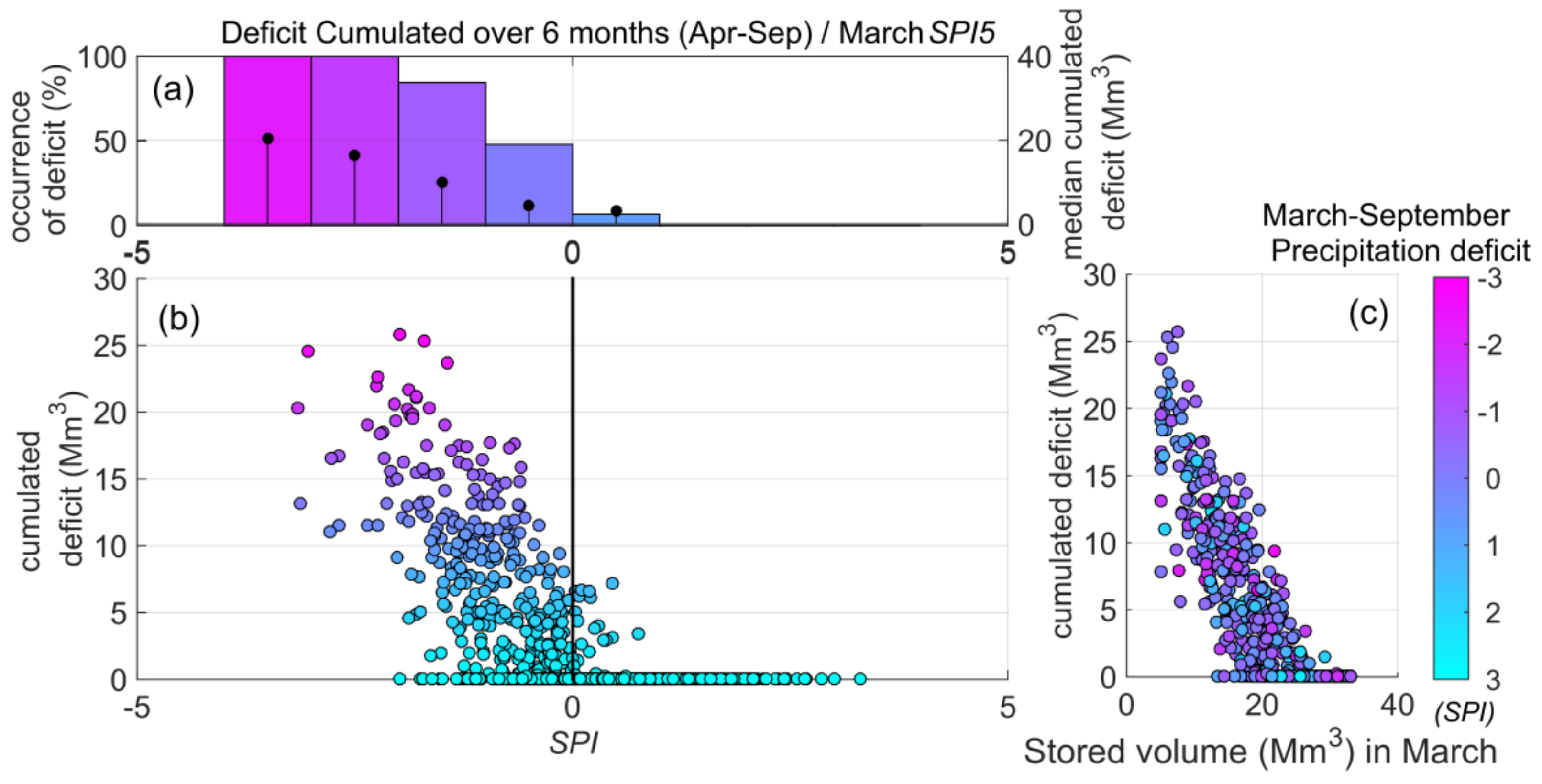
3.5. Support to Early-Warning (SEW)

In order to discuss the analysis performed through the SEW module, March has been taken into account as the month of analysis. This choice is related to two main aspects: (1) The highest precipitation rates occur in all the three case studies during the cold months (from late autumn to early spring); moreover, the related inflow to the reservoir is almost null during summer at both Ridracoli and Occhito, while at Lake Maggiore the variability of the monthly discharge during summer is low (the variation coefficients being 0.40 and 0.25 in July and August, compared to 0.90 and 0.74 in October and November). (2) The water demand is generally higher during the late spring and summer months, due to irrigation and/or the touristic season. This implies that an assessment of possible conditions of shortage and the consequent possible mitigation measures should be suitably undertaken at least in early spring. Of course, the proposed method of analysis can be extended to any month of the year.
The SEW module estimates the precipitation conditions occurred before the month of analysis (March) that potentially can lead to water shortage conditions in the following months. To this goal, an overview plot showing all the possible combination of SPI aggregation scales (from 1 to 12 antecedent months) and forecast window (from 1 to 12 future months) is delivered and analyzed. Therefore, as an example, the subplot (SPI3, DEF4) relates the precipitation cumulated over the trimester Jan-Feb-Mar to the deficit over the period Apr-May-Jun-Jul (similarly for the other subplots). In Figure 9, the overview plots show as a maximum the aggregation time scale for precipitation N = 6 months (thus considering precipitation from October to March) and as a maximum time window of forecast M = 6 months (from April to September). The complete figure, including all the possible 144 combinations (12 aggregation scales for SPI times 12 forecast windows) is not presented for clarity reasons.
The basic idea of the SEW analysis is that the higher the number of failure episodes for negative values of SPIn, the more effective will be the ability of such an index to forecast failures over the next M months. Moreover, the more the points on each graph are structured along a straight line, the more it is possible to predict the intensity of future deficits.
A visual inspection of Figure 9 suggests that forecast at six months (DEF6) is feasible for Ridracoli and Occhito, as plots appear well structured, while the forecast for Maggiore Lake over the same time window is not possible. The structure of the plots for both Ridracoli and Occhito leads us to conclude that for the two considered case studies, if winter precipitation (from October or November to March) is above the mean, the system is able to satisfy the entire water demand, whatever the spring and summer precipitation. The distribution of the deficit for SPI5 ≤ 0 (or SPI6 ≤ 0) appears to be well structured both at Ridracoli and Occhito. Approximately, the higher the negative precipitation anomaly, the stronger the probability to have a higher water deficit in the reservoir. Of course, such a structure appears to be more effective for early-warning as the time window of the forecast is reduced. Let us stress, as an example, the forecast ability of SPI6 at Occhito when the forecast window is reduced to 4 months ((SPI6, DEF4) in Figure 9c): the majority of the points for SPI6 ≤ 0 are aligned along a straight line, indicating the likely intensity of a future deficit.
The same analysis performed on the Lake Maggiore plots (Figure 9a) indicates that, for long forecast time windows (e.g., ≥5 months considering March as reference month), the capability to operate as an early-warning for future deficit is not consistent. The cloud of points for such timeframes appear not to be structured no matter the aggregation time scale that is taken into account for the precipitation. A large number of failure events occur also for SPI6 > 0, which means that the ability of the system to perform satisfactorily until the end of the irrigation season (August or September) strongly depends on the spring and/or summer precipitation. More information can be inferred only by reducing the forecast horizon. Considering, such as an example, a 3-months window, the precipitation of the last two months (SPI2) can be adopted as an early-warning for the next 3-months, as for SPI2 > 0 only few failures are shown. Similar considerations can be done concerning the forecast ability of SPI3 and SPI4 (for the same 3-months window of analysis). It is worth noting that increasing the time scale of the precipitation index (SPI5 and SPI6) does not necessarily improve the forecast capacity.
Results shown in Figure 9 can be analyzed from a quantitative perspective in order to obtain information on possible management actions in case of forecasted shortage episodes. To this goal, the Cohen’s k has been computed for each pair SPI (predictor)—forecast window (predictand). Figure 10 (from a to c panels) shows the Cohen’s k for each case study. The overview presented in Figure 10d reports the contour lines of the Cohen’s k coefficients, as well as the contour lines of the correlation of the regression coefficients computed accordingly to the methodology presented in Section 2.1.5. Figure 10 can be considered a summary of the main prediction performances for each case study.
Cohen’s k and r give different information. Cohen’s k quantifies the ability to forecast the occurrence of failure episodes, therefore it is strongly affected by both the number of true positives (failures correctly predicted) and the number of false positives (null deficit for SPI < SPImt as in the example of Figure 3). The correlation coefficient (r) measures the ability to forecast the intensity of the deficit as a function of the antecedent SPI when the failure occurs. It is also an assessment of the influence of the precipitation after the reference month on the future deficit intensity. From this perspective, it is a measure of the resilience of the system.
For most of the pairs (SPIn, DEFm) the management threshold SPImt is equal to 0. Few cases (6 in total) at Occhito are characterized by management thresholds lower than 0, all of them for small forecast windows (2 or 3 months) and long aggregation scale of SPI (5 or 6 months).
Cohen’s k is well structured over the space (SPIn, DEFm) for all the three case studies, as it is possible to find a pair for which this coefficient is maximized. It is worth noting from Figure 10 that no relative minimum or maximum can be found (surfaces are convex). A summary of the Cohen’s k statistics and regression coefficient is presented in Table 3.
The highest values of Cohen’s k are computed for Ridracoli. This is due to the specific features of such a reservoir. In fact, on the one hand Ridacoli is a relatively small reservoir, on the other hand the inflow to it takes place basically during the cold months (from late autumn to early spring). This implies that knowing the past precipitation at the beginning of spring allows us to correctly forecast future failures, maximizing the percentage of true positives and minimizing the percentage of false positives. SPI6 appears to be the best predictor for a time window of 7 months (therefore including the summer months). The contour line 0.6 of the correlation coefficient (r) over the (SPIn, DEFm) space (Figure 10d), shows that increasing the SPI time scale as predictor does not add new information, as the internal area is very narrow and aligned along the DEF7 class. The contour line of the regression coefficient is almost overlapped to the contour line of the Cohen’s k, implying that the maximum ability to predict the occurrence of deficit coincides with the maximum ability to predict the failure’s intensity.
This is not the case for Occhito, although it is possible to find a pair (SPIn, DEFm) that maximizes the Cohen’s k, its absolute value is lower with respect to Ridracoli. This is due to the higher number of false positives, which is related to the great volume of such a reservoir that strongly limits the number of failures. It is interesting to note from Figure 10d that the area bounded by the Cohen’s k contour line 0.35 is approximately a square. Increasing the forecast time window from 7 to 12 months does not affect the performance of the predictor, provided that the aggregation time scale for the SPI is increased from 5 to 10 months. In opposition to what has been observed for Ridracoli, the maximum of the correlation coefficient area does not overlap to the maximum of the Cohen’s k, although it is much higher. From a management perspective, this means that even if it is possible to perform forecasts in terms of the probability of occurrence over long time windows (from 7 to 12), predictions of a deficit’s intensity are less feasible for those periods. Decreasing the analysis windows (to 3 or 4 months) improves the regression coefficients (i.e., it improves the prediction of the intensity of deficit), but significantly degrades the performance in predicting the occurrence, due to the high number of false positives.
Analysis of the Cohen’s k for Lake Maggiore (Figure 10a) shows that predicting future failures in terms both of occurrence and the intensity of the deficit is definitively less feasible than at Ridracoli and Occhito, both the maximum Cohen’s k and maximum regression coefficients are lower than at Ridracoli and Occhito. Maxima for both indices are obtained for short time windows (2 to 3 months), considering 4 months as a time aggregation scale of SPI. As already stressed before, this is basically due to the high value of the connected demand with respect to the reservoir maximum capacity of the lake (Table 1, RMC/MAD = 0.05). Moreover, the high value of the annual inflow with respect to the reservoir maximum capacity (Table 1, RMC/MAI = 0.03) makes the lake more prone to overflow episodes, limiting the storage capability and, as a consequence, the performance of the early-warning system.
Results from the SEW procedure allows us to conclude that for Ridracoli and Occhito it is possible to early detect future conditions of shortage over time scales of 6 months, considering the SPI6 or SPI7 computed in March as predictor. Increasing the aggregation time scale of SPI allows to extend the forecast time scale only for Occhito, while at Ridracoli increasing the SPI does not add new information on early warning. The forecast window is much shorter for Lake Maggiore, whatever the chosen time scale for SPI aggregation, due to the limited ability of the Lake to store water (whose regulation levels are established by law) and, as a consequence, to manage the supply over time scales longer than a few months.

4. Conclusions

In this paper, a robust tool is presented for the analysis of water shortage risk in water supply systems constituted by a reservoir connected to multiple water demand systems. The final goal of the proposed methodology, implemented in a computational software named INOPIA, is the identification of “management triggers” for the implementation of specific mitigation measures based on water-saving policies. In this work, the emphasis is given on defining a robust system of indicators, according to the EU standards, to support drought risk management as a tool to promote participative processes and achieve effectively implemented mitigation measures. To this aim, the presented methodology has been based on a preliminary end-users’ consultation.
The proposed tool allows for the quantification of the risk of shortage for a given WSS. Such a quantification is carried out through a statistical analysis of the time series of failures. The latter are obtained by a guided procedure driving the simulation of the inflows to the reservoir from precipitation data through a self-calibrating multilinear regression model (SPI-Q model). Time series of failures are analyzed by means of reliability-resilience-vulnerability metrics, able to capture and quantify extreme events through standardized indices. Then, results are quantitatively analyzed in order to identify “management triggers” for the implementation of specific mitigation measures based on allocation policies. Main potentialities of the proposed tool can be summarized as follows:
  • The calibration procedure performed through the SPI-Q model is based only on precipitation and discharge data. The minimal number of parameters along with the self-calibration procedure allows the implementation and comprehension of the hydrological model also by non-expert users. Moreover, although it is statistically-based, it maintains the physical meaning of the parameters. Despite model simplicity, the simulations performed on the three Italian case studies showed the goodness of the method for studying occurrence of failures.
  • The method adopted to generate scenarios allows for the simulation of a discharge time series based on both the time series of precipitation (i.e., from medium term weather forecast) and directly on the Standardized Precipitation Indices time series, which is particularly useful when implementing climate change scenarios from a General Circulation Models (GCM) output. The main limit of the proposed approach relies on the basic assumption that catchment response to the precipitation regime is time invariant.
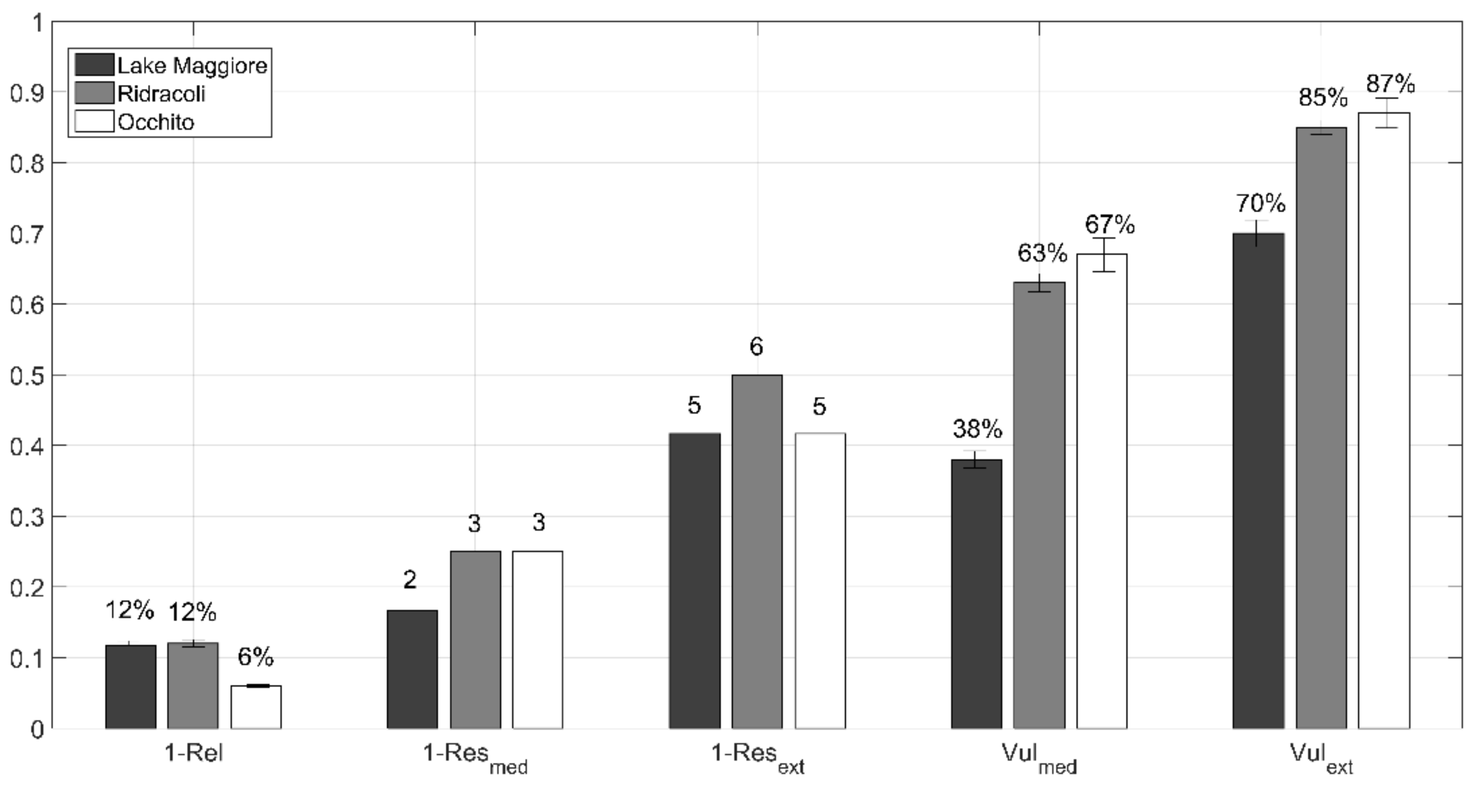
  • A new formulation of the reliability-resilience-vulnerability metrics has been tested on the three case studies (a previous discussion on this new formulation solely on the case of the Ridracoli reservoir can be found in [49]). The use of standardized indices allowed for a quick comparison among water systems regardless of the differences in size, climate, meteorological, and hydrological regimes of the basins and reservoirs.
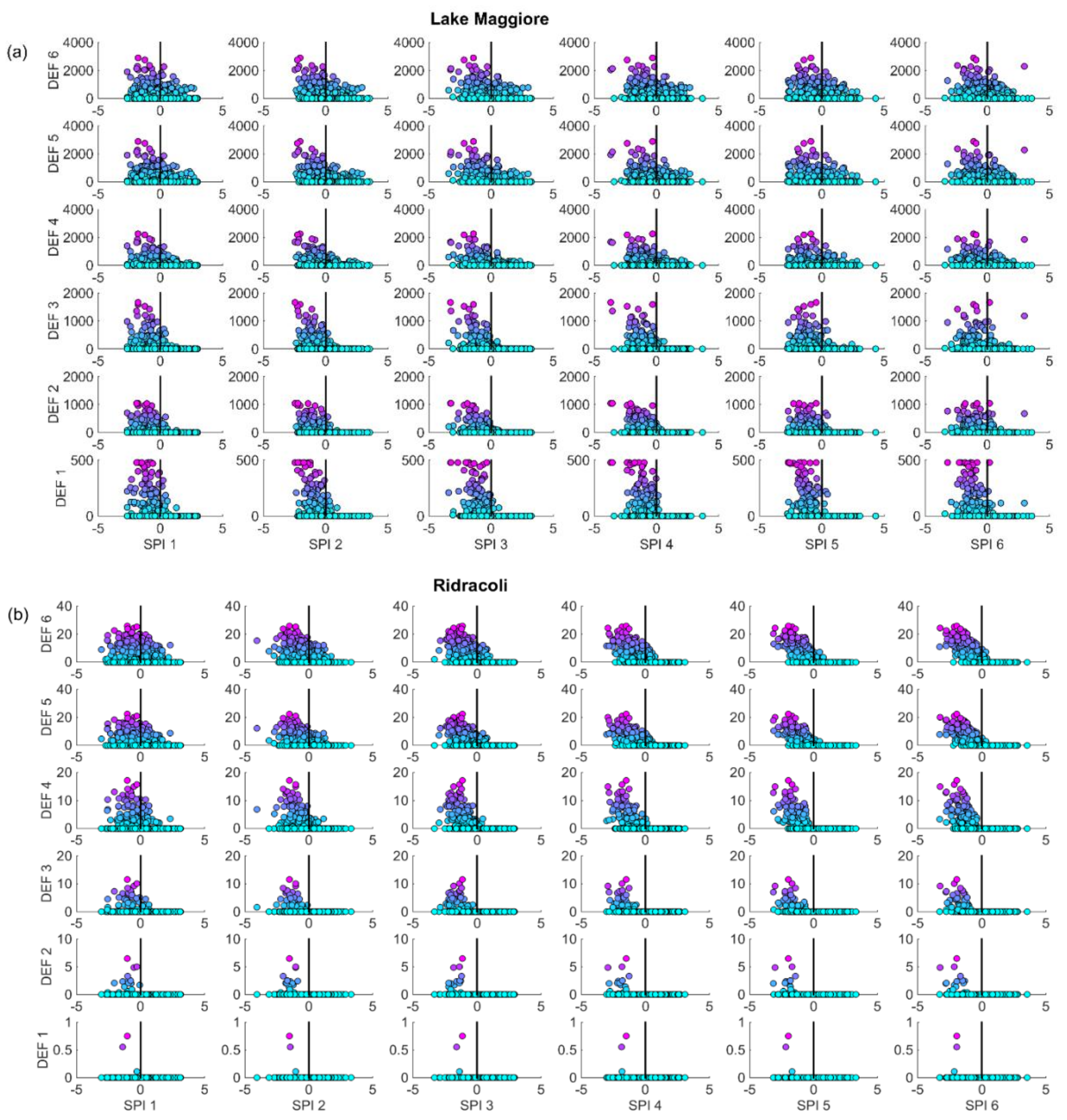
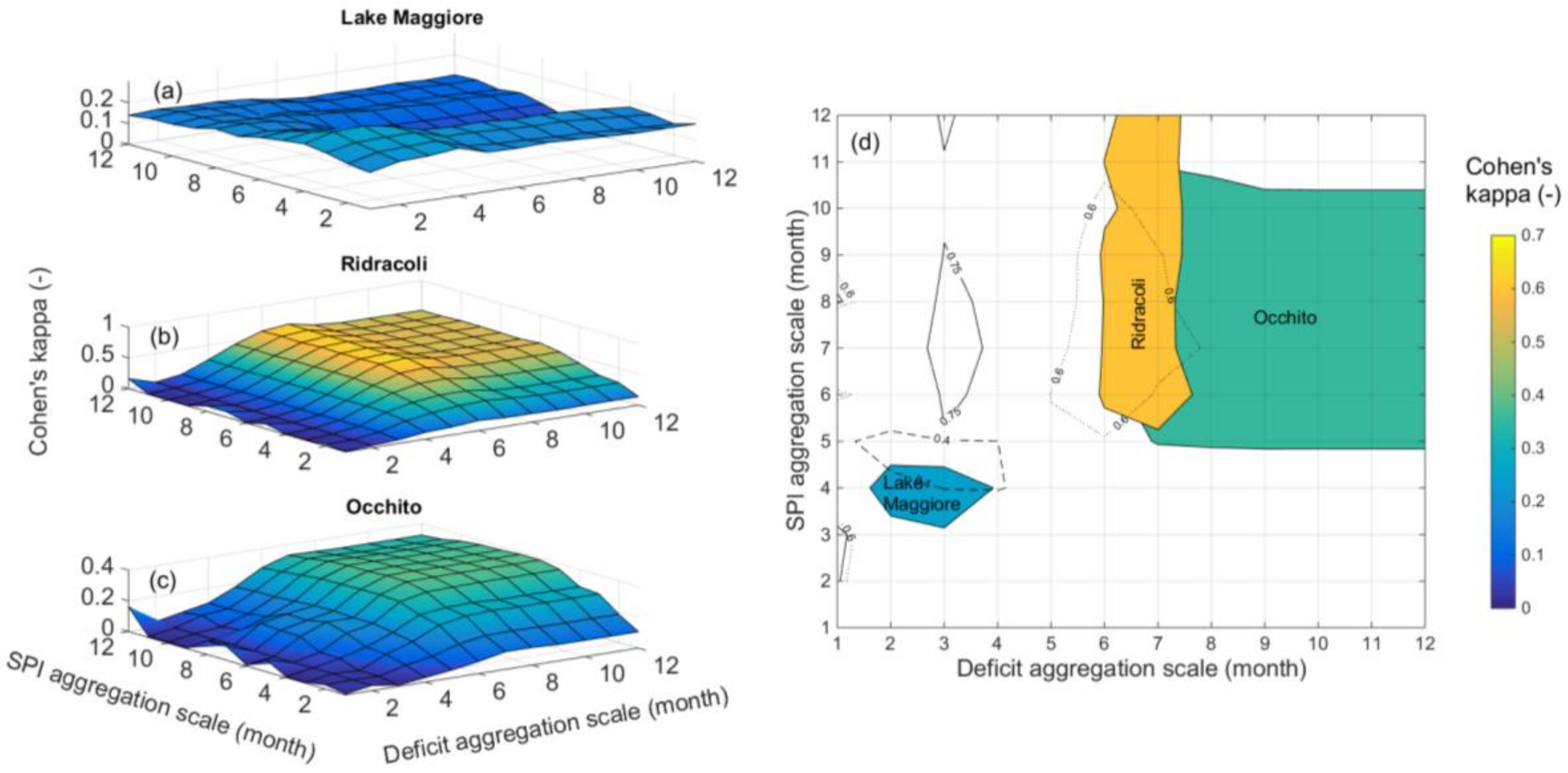
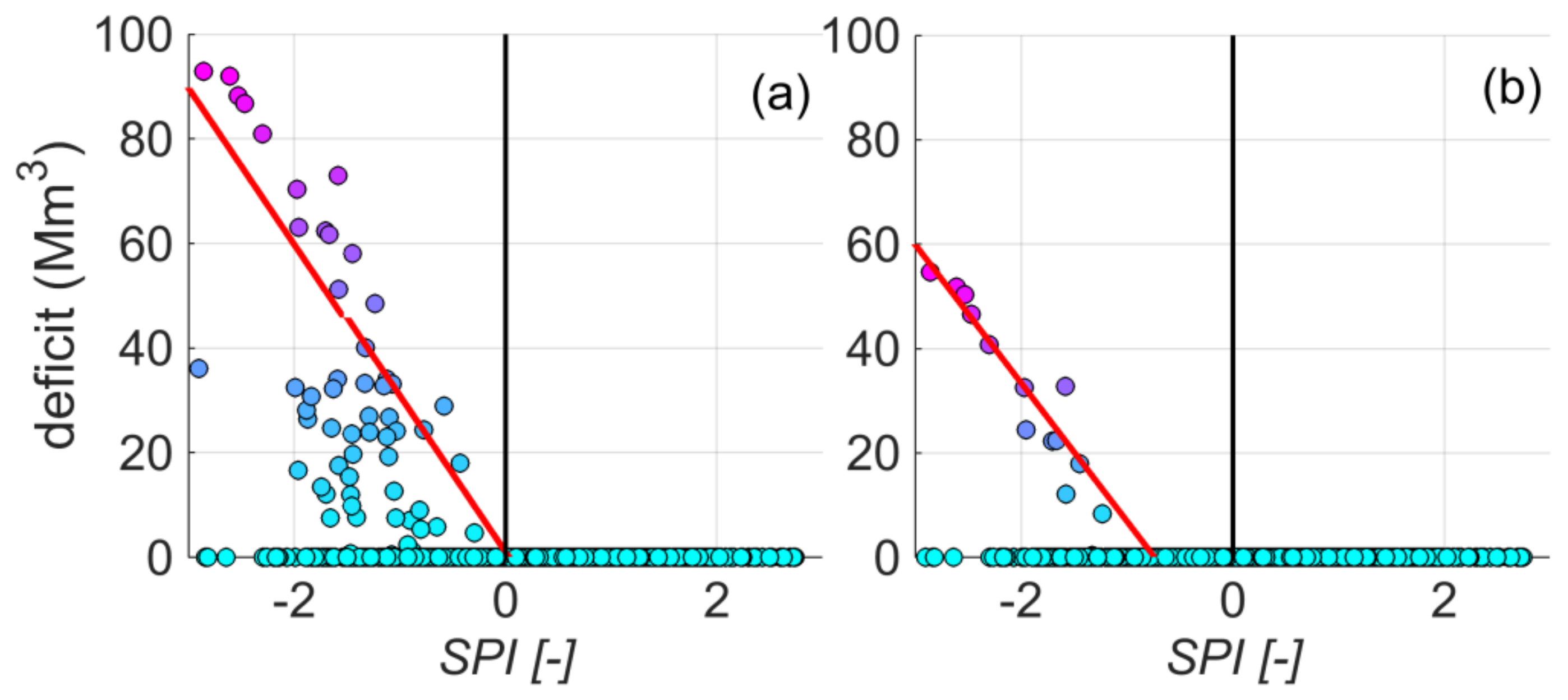
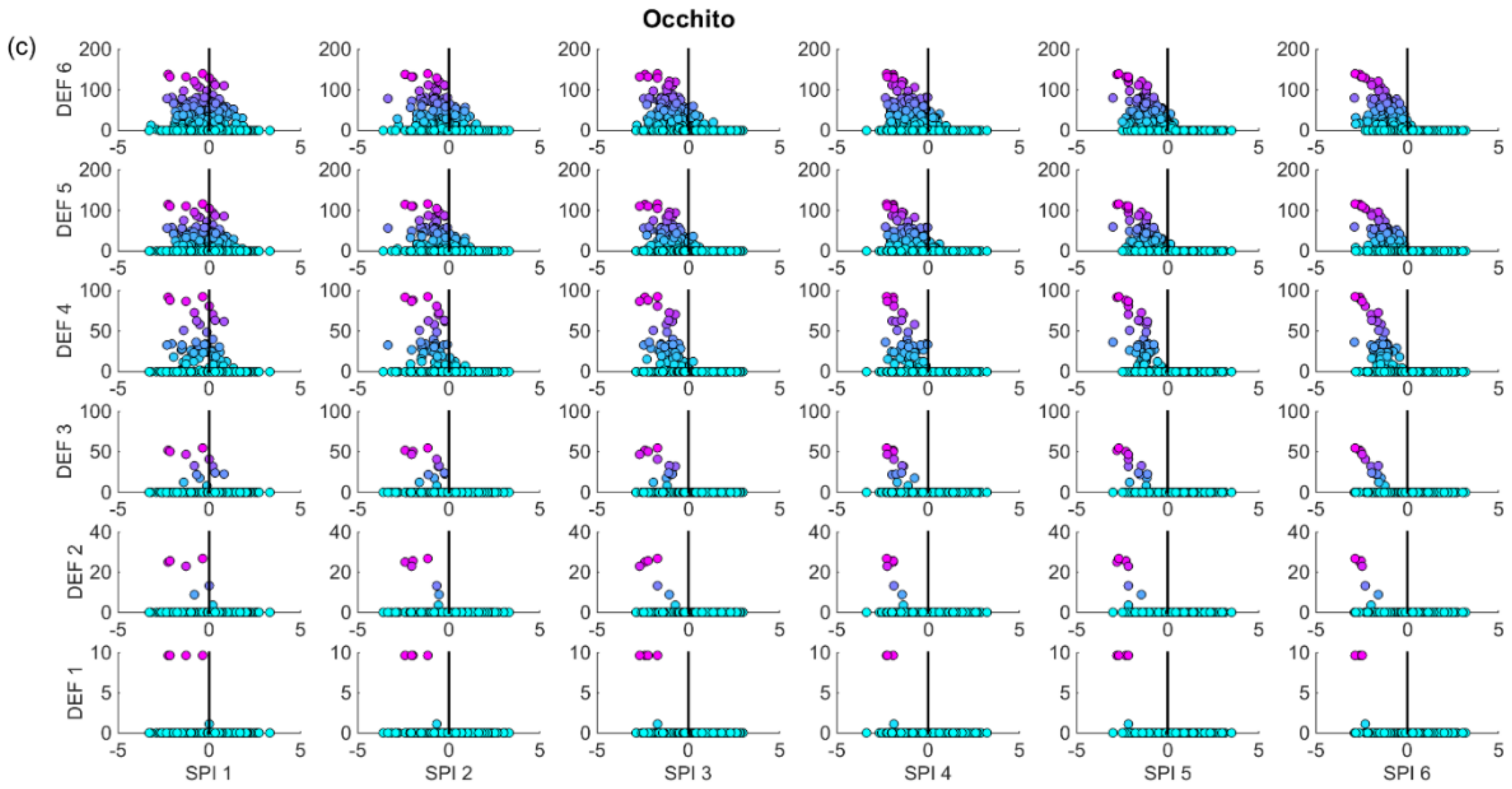
  • The Support to Early-Warning procedure relates the precipitation regime, represented by the SPI at different time scales, to the simulated deficit volumes computed over the m following months. This kind of representation allows a user to qualitatively identify possible early-warnings by analyzing the antecedent precipitation conditions that can potentially lead to shortage conditions over a future time window assigned by the user. A quantitative method to analyze the output from the SEW module and to identify possible “management triggers” is proposed. It is based on the Cohen’s coefficient and allows for ranking the predictor in terms of antecedent precipitation (SPI) and forecast time scale. Possible management options based on different future water allocation schemes (both in time and quantity) can be suggested based on the linear regression of the forecasted deficit versus the antecedent standardized precipitation indices.
It is important to stress that the current version of the proposed tool, developed in collaboration with the National Civil Protection Department of Italy, has been adopted by the Permanent Observatories of the Central and South Apennine Hydrographic Districts as its early-warning system for WSS management under water scarcity conditions. However, it is worth noting that in the current level of development, INOPIA can be adopted to analyze WSSs constituted by one single reservoir fed by surface waters. Future developments, already ongoing, will be addressed to extend the proposed approach to water supply systems constituted by multiple surface reservoirs, possibly interconnected, supplying multiple users. This will allow for analyzing the drought vulnerability of single components of complex WSSs, permitting the exploration of a wider range of management options.
Finally, the proposed tool, once fully developed, can be adopted and added as part of Water Safety Plans in the “System assessment”, “Monitoring”, and “Management and Communication” sections of the WMO guidelines [34].

Author Contributions

Conceptualization, E.R. and A.D.; Methodology, E.R., N.G. and F.S.; Investigation, E.R., N.G., R.G., A.B.P., I.P. and F.S.; Writing-Original Draft Preparation, E.R., N.G., A.B.P., F.S.; Writing-Review & Editing, A.B.P., R.G. and I.P.

Funding

This research was funded by the National Civil Protection of Italy through the Agreement between Civil Protection Department and Water Research Institute, aiming at developing Methodologies for monitoring water resources and forecasting water shortage conditions.

Acknowledgments

The authors wish to thank Consorzio del Ticino, Romagna Acque—Società delle Fonti s.r.l and Consorzio della Capitanata for kindly sharing the available data and technically supporting this research. Precipitation data were provided by Scuola Universitaria Professionale della Svizzera Italiana (www.supsi.ch/) and ARPA Piemonte (http://www.arpa.piemonte.gov.it/) for the Lake Maggiore case study, ARPA Emilia-Romagna (https://www.arpae.it/) for the Ridracoli case study, and Centro Funzionale Regione Puglia (http://www.protezionecivile.puglia.it/centro-funzionale) for the Occhito case study.

Conflicts of Interest

The authors declare no conflict of interest.

References

  1. European Commission. Water Scarcity and Droughts Expert Network Drought Management Plan Report; Including Agricultural, Drought Indicators and Climate Change Aspects; Technical Report; EU: Maastricht, The Netherlands, 2008. [Google Scholar]
  2. Karavitis, C.A.; Tsesmelis, D.E.; Skondras, N.A.; Stamatakos, D.; Alexandris, S.; Fassouli, V.; Vasilakou, C.G.; Oikonomou, P.D.; Gregorič, G.; Grigg, N.S.; et al. Linking drought characteristics to impacts on a spatial and temporal scale. Water Policy 2014, 16, 1172–1197. [Google Scholar] [CrossRef]
  3. Wang, D.; Hejazi, M.; Cai, X.; Valocchi, A.J. Climate change impact on meteorological, agricultural, and hydrological drought in central Illinois. Water Resour. Res. 2011, 47, W09527. [Google Scholar] [CrossRef]
  4. Van Loon, A. Hydrological drought explained. WIREs Water 2015, 2, 359–392. [Google Scholar] [CrossRef] [Green Version]
  5. Lopez-Moreno, J.; Vicente-Serrano, S.; Beguerıa, S.; Garcıa-Ruiz, J.; Portela, M.; Almeida, A. Downstream propagation of hydrological droughts in highly regulated transboundary rivers: The case of the Tagus river between Spain and Portugal. Water Resour. Res. 2009, 45, W02405. [Google Scholar]
  6. Garrote, L.; Martin-Carrasco, F.; Flores-Montoya, F.; Iglesias, A. Linking Drought Indicators to Policy Actions in the Tagus Basin Drought Management Plan. Water Resour. Manag. 2007, 21, 873–882. [Google Scholar] [CrossRef]
  7. Hao, Z.; Hao, F.; Singh, V.P.; Xia, Y.; Ouyang, W.; Shen, X. A theoretical drought classification method for the multivariate drought index based on distribution properties of standardized drought indices. Adv. Water Resour. 2016, 92, 240–247. [Google Scholar] [CrossRef]
  8. Gustard, A.; Young, A.; Rees, G.; Holmes, M. Operational hydrology. In Hydrological Drought. Processes and Estimation Methods for Streamflow and Groundwater; Tallaksen, L., van Lanen, H.A.J., Eds.; Elsevier: Amsterdam, The Netherlands, 2004; pp. 455–498. [Google Scholar]
  9. Wilhite, D.A.; Hayes, M.J.; Svoboda, M.D. Drought monitoring and assessment: Status and trends in the United States. In Drought and Drought Mitigation in Europe; Vogt, J.V., Somma, F., Eds.; Kluwer Academic Publishers: Amsterdam, The Netherlands, 2000; pp. 149–160. [Google Scholar]
  10. Wilhite, D.A.; Svoboda, M.D.; Hayes, M.J. Understanding the complex impacts of drought: A key to enhancing drought mitigation and preparedness. Water Resour. Manag. 2007, 21, 763–774. [Google Scholar] [CrossRef] [Green Version]
  11. Svoboda, M.; LeComte, D.; Hayes, M.; Heim, R.; Gleason, K.; Angel, J.; Rippey, B.; Tinker, R.; Palecki, M.; Stooksbury, D.; et al. The drought monitor. Bull. Am. Meteorol. Soc. 2002, 83, 1181–1190. [Google Scholar] [CrossRef]
  12. Mens, M.J.P.; Gilroy, K.; Williams, D. Developing system robustness analysis for drought risk management: An application on a water supply reservoir. Nat. Hazard. Earth Syst. Sci. 2015, 15, 1933–1940. [Google Scholar] [CrossRef]
  13. Wu, W.; Maier, H.R.; Dandy, G.C.; Leonard, R.; Bellette, K.; Cuddy, S.; Maheepala, S. Including stakeholder input in formulating and solving real-world optimisation problems: Generic framework and case study. Environ. Model. Softw. 2016, 79, 197–213. [Google Scholar] [CrossRef]
  14. Voinov, A.; Kolagani, N.; McCall, M.K.; Glynn, P.D.; Kragt, M.E.; Ostermann, F.O.; Pierce, S.A.; Ramu, P. Modelling with stakeholders—Next generation. Environ. Model. Softw. 2016, 77, 196–220. [Google Scholar] [CrossRef]
  15. Giacomelli, P.; Rossetti, A.; Brambilla, M. Adapting water allocation management to drought scenarios. Nat. Hazard. Earth. Syst. Sci. 2008, 8, 293–302. [Google Scholar] [CrossRef] [Green Version]
  16. Westphal, K.S.; Laramie, R.L.; Borgatti, D.; Stoops, R. Drought management planning with economic and risk factors. J. Water Resour. Plan. Manag. 2007, 133, 351–362. [Google Scholar] [CrossRef]
  17. Giordano, R.; Preziosi, E.; Romano, E. Integration of local and scientific knowledge to support drought impact monitoring: Some hints from an Italian case study. Nat. Hazards 2013, 69, 523–544. [Google Scholar] [CrossRef]
  18. Giordano, R.; D’Agostino, D.; Apollonio, C.; Scardigno, A.; Pagano, A.; Portoghese, I.; Lamaddalena, N.; Piccinni, A.F.; Vurro, M. Evaluating acceptability of groundwater protection measures under different agricultural policies. Agric. Water Manag. 2015, 147, 54–66. [Google Scholar] [CrossRef]
  19. Wilhite, D.A. Drought Monitoring as a Component of Drought Preparedness Planning. In Coping with Drought Risk in Agriculture and Water Supply Systems. Drought Management and Policy Development in the Mediterranean; Iglesias, C.A., Garrote, L., Cancelliere, A., Cubillo, F., Wilhite, D.A., Eds.; Springer: Amsterdam, The Netherlands, 2009. [Google Scholar]
  20. Botterill, L.C.; Hayes, M.J. Drought triggers and declarations: Science and policy considerations for drought risk management. Nat. Hazards 2012, 64, 139–151. [Google Scholar] [CrossRef]
  21. Ceppi, A.; Ravazzani, C.; Corbari, C.; Meucci, S.; Pala, F.; Salerno, R.; Meazza, G.; Chiesa, M.; Mancini, M. Real Time Drought Forecasting System for Irrigation Management. Procedia Environ. Sci. 2013, 19, 776–784. [Google Scholar] [CrossRef]
  22. Hao, Z.; Hao, F.; Singh, V.P.; Ouyang, W.; Cheng, H. An integrated package for drought monitoring, prediction and analysis to aid drought modeling and assessment. Environ. Model. Softw. 2017, 91, 199–209. [Google Scholar] [CrossRef]
  23. Esfahanian, E.; Pouyan Nejadhashemi, A.; Abouali, M.; Adhikari, U.; Zhang, Z.; Daneshvar, F.; Herman, M.R. Development and evaluation of a comprehensive drought index. J. Environ. Manag. 2017, 185, 31–43. [Google Scholar] [CrossRef] [PubMed]
  24. Liu, Y.; Gupta, H.; Springer, E.; Wagener, T. Linking science with environmental decision making: Experiences from an integrated modeling approach to supporting sustainable water resources management. Environ. Model. Softw. 2008, 23, 846–858. [Google Scholar] [CrossRef]
  25. Preziosi, E.; Del Bon, A.; Romano, E.; Petrangeli, A.B.; Casadei, S. Vulnerability to drought of a complex water supply system. The upper Tiber basin case study (Central Italy). Water Resour. Manag. 2013, 27, 4655–4678. [Google Scholar] [CrossRef]
  26. Yan, D.; Weng, B.; Wang, G.; Wang, H.; Yin, J.; Bao, S. Theoretical framework of generalized watershed drought risk evaluation and adaptive strategy based on water resources system. Nat. Hazards 2014, 73, 259–276. [Google Scholar] [CrossRef]
  27. Weng, B.S.; Yan, D.H.; Wang, H.; Liu, J.H.; Yang, Z.Y.; Qin, T.L.; Yin, J. Drought assessment in the Dongliao River basin: Traditional approaches vs. generalized drought assessment index based on water resources systems. Nat. Hazard. Earth Syst. Sci. 2015, 15, 1889–1906. [Google Scholar] [CrossRef]
  28. Ravazzani, G.; Barbero, S.; Salandin, A.; Senatore, A.; Mancini, M. An integrated Hydrological Model for Assessing Climate Change Impacts on Water Resources of the Upper Po River Basin. Water Resour. Manag. 2015, 29, 1193–1215. [Google Scholar] [CrossRef]
  29. Zare, F.; Elsawah, S.; Iwanaga, T.; Jakeman, A.J.; Pierce, S.A. Integrated water assessment and modelling: A bibliometric analysis of trends in the water resource sector. J. Hydrol. 2017, 552, 765–778. [Google Scholar] [CrossRef]
  30. World Health Organization. Guidelines for Drinking-Water Quality, 4th ed.; WHO: Geneva, Switzerland, 2011; ISBN 978-92-4-154815-1. [Google Scholar]
  31. Pietrucha-Urbanik, K. Multidimensional Comparative Analysis of Water Infrastructures Differentiation, Environmental Engineering IV; Pawłowski, A., Dudzińska, M.R., Pawłowski, L., Eds.; Taylor & Francis Group: London, UK, 2013; pp. 29–34. [Google Scholar]
  32. Pietrucha-Urbanik, K. Assessing the costs of losses incurred as a result of failure. In Dependability Engineering and Complex Systems; Zamojski, W., Mazurkiewicz, J., Sugier, J., Walkowiak, T., Kacprzyk, J., Eds.; Advances in Intelligent Systems and Computing; Springer: Amsterdam, The Netherlands, 2016. [Google Scholar]
  33. Pietrucha-Urbanik, K.; Tchorzewska-Cieslak, B. Water Supply System operation regarding consumer safety using Kohonen neural network. In Safety, Reliability and Risk Analysis: Beyond the Horizon; Steenbergen, R.D.J.M., Miraglia, S., Eds.; Taylor & Francis Group: London, UK, 2014; pp. 1115–1120. [Google Scholar]
  34. Tchorzewska-Cieslak, B.; Rak, J. Method of identification of operational states of water supply system. In Proceedings of the 3rd Congress of Environmental Engineering, Lublin, Poland, 13–16 September 2009; Environmental Engineering III. Pawlowski, L., Dudzinska, M.R., Pawlowski, A., Eds.; Taylor & Francis Group: London, UK, 2010; pp. 521–526. [Google Scholar]
  35. Andreu, J.; Capilla, J.; Sanchìs, E. AQUATOOL, a generalised decision-support system for water-resources planning and operational management. J. Hydrol. 1996, 177, 269–291. [Google Scholar] [CrossRef]
  36. Labadie, J.W.; Baldo, M.L.; Larson, R. MODSIM: Decision Support System for River Basin Management: Documentation and User Manual; Colorado State University and U.S. Bureau of Reclamation: Ft Collins, CO, USA, 2000. [Google Scholar]
  37. Ahn, S.R.; Jeong, J.H.; Kim, S.J. Assessing drought threats to agricultural water supplies under climate change by combining the SWAT and MODSIM models for the Geum River basin, South Korea. Hydrol. Sci. J. 2016, 61, 2740–2753. [Google Scholar] [CrossRef]
  38. Chhuon, K.; Herrera, E.; Nadaoka, K. Application of Integrated Hydrologic and River Basin Management Modeling for the Optimal Development of a Multi-Purpose Reservoir Project. Water Resour. Manag. 2016, 30, 3143–3157. [Google Scholar] [CrossRef]
  39. SEI (Stockholm Environment Institute). WEAP: Water Evaluation and Planning System-User Guide; Stockholm Environment Institute: Boston, MA, USA, 2001. [Google Scholar]
  40. Delft Hydraulics. River Basin Planning and Management Simulation Program. In Proceedings of the IEMSs Third Biennial Meeting: Summit on Environmental Modelling and Software, Burlington, VT, USA, 9–13 July 2006; Voinov, A., Jakeman, A.J., Rizzoli, A.E., Eds.; International Environmental Modelling and Software Society: Burlington, VT, USA, 2006. [Google Scholar]
  41. Sechi, G.M.; Sulis, A. Water system management through a mixed optimization-simulation approach. J. Water Resour. Plan. Manag. 2009, 135, 160–170. [Google Scholar] [CrossRef]
  42. Casadei, S.; Pierleoni, A.; Bellezza, M. Integrated Water Resources Management in a Lake System: A Case Study in Central Italy. Water 2016, 8, 570. [Google Scholar] [CrossRef]
  43. De Lange, W.J.; Prinsen, G.F.; Hoogewoud, J.C.; Veldhuizen, A.A.; Verkaik, J.; Oude Essink, G.H.P.; van Walsum, P.E.V.; Delsman, J.R.; Hunink, J.C.; Massop, H.T.L.; et al. An operational, multi-scale, multi-model system for consensus-based, integrated water management and policy analysis: The Netherlands Hydrological Instrument. Environ. Model. Softw. 2014, 59, 98–108. [Google Scholar] [CrossRef]
  44. Sulis, A.; Sechi, G.M. Comparison of generic simulation models for water resource systems. Environ. Model. Softw. 2013, 40, 214–225. [Google Scholar] [CrossRef]
  45. McKee, T.B.; Doesken, N.J.; Kleist, K. The relationship of drought frequency and duration to time scale. In Proceedings of the 8th Conference on Applied Climatology, Anaheim, CA, USA, 17–22 January 1993; American Meteor Society: Boston, MA, USA, 1993. [Google Scholar]
  46. Romano, E.; Preziosi, E.; Petrangeli, A.B. Spatial and Time Analysis of Rainfall in the Tiber River Basin (Central Italy) in relation to Discharge Measurements (1920–2010). Procedia Environ. Sci. 2011, 7, 258–263. [Google Scholar] [CrossRef]
  47. Romano, E.; Preziosi, E. Precipitation pattern analysis in the Tiber River basin (Central Italy) using standardized indices. Int. J. Climatol. 2013, 33, 1781–1792. [Google Scholar] [CrossRef]
  48. Romano, E.; Del Bon, A.; Petrangeli, A.B.; Preziosi, E. Generating synthetic time series of springs discharge in relation to standardized precipitation indices. Case study in Central Italy. J. Hydrol. 2013, 507, 86–99. [Google Scholar] [CrossRef]
  49. Guyennon, N.; Romano, E.; Portoghese, I. Long-term climate sensitivity of an integrated water supply system: The role of irrigation. Sci. Total Environ. 2016, 565, 68–81. [Google Scholar] [CrossRef] [PubMed]
  50. Romano, E.; Guyennon, N.; Del Bon, A.; Petrangeli, A.B.; Preziosi, E. Robust method to quantify the risk of shortage for water supply systems. J. Hydrol. Eng. 2017, 22, 04017021. [Google Scholar] [CrossRef]
  51. Guyennon, N.; Salerno, F.; Portoghese, I.; Romano, E. Climate change Adaptation in a Mediterranean semi-arid catchment: Testing Managed Aquifer Recharge and Increased Surface Reservoir Capacity. Water 2017, 9, 689. [Google Scholar] [CrossRef]
  52. Lloyd-Hughes, B.; Saunders, M.A. A drought climatology for Europe. Int. J. Climatol. 2002, 22, 1571–1592. [Google Scholar] [CrossRef] [Green Version]
  53. Paulo, A.; Martins, D.; Santos Pereira, L. Influence of Precipitation Changes on the SPI and Related Drought Severity. An Analysis Using Long-Term Data Series. Water Resour. Manag. 2016, 30, 5737–5757. [Google Scholar] [CrossRef] [Green Version]
  54. Rossi, S.; Niemeyer, S. Drought Monitoring with estimates of the Fraction of Absorbed Photosynthetically-active Radiation (fAPAR) derived from MERIS. In Remote Sensing for Drought: Innovative Monitoring Approaches; Wardlow, B., Anderson, M., Verdin, J., Eds.; CRC Press-Taylor & Francis: Boca Raton, FL, USA, 2012; pp. 95–116. [Google Scholar]
  55. Sepulcre-Canto, G.; Horion, S.; Singleton, A.; Carrao, H.; Vogt, J. Development of a Combined Drought Indicator to detect agricultural drought in Europe. Nat. Hazard. Earth Syst. Sci. 2012, 12, 3519–3531. [Google Scholar] [CrossRef] [Green Version]
  56. Bachmair, S.; Kohn, I.; Stahl, K. Exploring the link between drought indicators and impacts. Nat. Hazard. Earth. Syst. Sci. 2015, 15, 1381–1397. [Google Scholar] [CrossRef] [Green Version]
  57. Kjeldsen, T.R.; Rosbjerg, D. Choice of reliability, resilience and vulnerability estimators for risk assessments of water resources systems/Choix d’estimateurs de fiabilité, de résilience et de vulnérabilité pour les analyses de risqué de systèmes de ressources en eau. Hydrol. Sci. J. 2004, 49, 755–767. [Google Scholar] [CrossRef]
  58. Mortazavi, M.; Kuczera, G.; Cui, L. Multiobjective optimization of urban water resources: Moving toward more practical solutions. Water Resour. Res. 2012, 48, W03514. [Google Scholar] [CrossRef]
  59. Gomez-Beas, R.; Monino, A.; Polo, M.J. Development of a management tool for reservoirs in Mediterranean environments based on uncertainty analysis. Nat. Hazard. Earth Syst. Sci. 2012, 12, 1789–1797. [Google Scholar] [CrossRef] [Green Version]
  60. Asefa, T.; Clayton, J.; Adam, A.; Anderson, D. Performance evaluation of a water resources system under varying climatic conditions: Reliability, Resilience, Vulnerability and beyond. J. Hydrol. 2014, 508, 53–65. [Google Scholar] [CrossRef]
  61. Mortazavi-Naeini, M.; Kuczera, G.; Cui, L. Application of multiobjective optimization to scheduling capacity expansion of urban water resource systems. Water Resour. Res. 2014, 50, 4624–4642. [Google Scholar] [CrossRef]
  62. Hashimoto, T.; Stedinger, J.R.; Loucks, D.P. Reliability, resiliency, and vulnerability criteria for water resource system performance evaluation. Water. Resour. Res. 1982, 18, 14–20. [Google Scholar] [CrossRef] [Green Version]
  63. Xu, Z.; Jinno, K.; Kawamura, A.; Takesaki, S.; Ito, K. Performance risk analysis for Fukuoka water supply system. Water Resour. Manag. 1998, 12, 13–30. [Google Scholar] [CrossRef]
  64. Klise, K.A.; Bynum, M.; Moriarty, D.; Murray, R. A software framework for assessing the resilience of drinking water systems to disasters with an example earthquake case study. Environ. Model. Softw. 2017, 95, 420–431. [Google Scholar] [CrossRef]
  65. Merabtene, T.; Kawamura, A.; Jinno, K.; Olsson, J. Risk assessment for optimal drought management of an integrated water resources system using a genetic algorithm. Hydrol. Process. 2002, 16, 2189–2208. [Google Scholar] [CrossRef]
  66. Montaseri, M.; Adeloye, A.J. Critical period of reservoir systems for planning purposes. J. Hydrol. 1999, 224, 115–136. [Google Scholar] [CrossRef]
  67. Ben-David, A. A lot of randomness is hiding in accuracy. Eng. Appl. Artif. Intell. 2007, 20, 875–885. [Google Scholar] [CrossRef]
  68. Ben-David, A. About the relationship between ROC curves and Cohen’s kappa. Eng. Appl. Artif. Intell. 2008, 21, 874–882. [Google Scholar] [CrossRef]
  69. Yamijala, S.; Guikema, S.; Brumbelow, K. Statistical models for the analysis of water distribution system pipe break data. Reliab. Eng. Syst. Safe 2009, 94, 282–293. [Google Scholar] [CrossRef]
  70. Debon, A.; Carrion, A.; Cabrera, E.; Solano, H. Comparing risk of failure models in water supply network using ROC curves. Reliab. Eng. Syst. Safe 2010, 95, 43–48. [Google Scholar] [CrossRef]
  71. Fleiss, J.L. Statistical Methods for Rates and Proportions, 2nd ed.; John Wiley: New York, NY, USA, 1981; ISBN 0-471-26370-2. [Google Scholar]
Figure 1. Methodology flowchart. Colored ellipses refer to the steps of analysis of the tool INOPIA, described in details in Section 2.1.1, Section 2.1.2, Section 2.1.3, Section 2.1.4 and Section 2.1.5.
Water 10 00762 g001
Figure 2. Support-to-early warning graphical analysis. (a) Occurrence of deficit (colored bars, principal y axis) and median cumulated deficit (stems, secondary y axis) for each class of Standardized Precipitation Index (SPI). (b) Cumulated deficit for each shortage episode as a function of the correspondent SPI. Color code refers to the cumulated deficit. (c) Cumulated deficit over 6 months as a function of the volume stored in March. Color code refers to the SPI value. The example refers to the Ridracoli case study (month of analysis: March; predictor: SPI6; forecast time window: 5 months).
Water 10 00762 g002
Figure 3. Example of quantitative analysis of the SUPPORT TO EARLY-WARNING plots.
Water 10 00762 g003
Figure 4. (a) Location of the case studies. (b) Lake Maggiore. (c) Ridracoli. (d) Occhito.
Water 10 00762 g004
Figure 5. Precipitation (left y-axis) and standardized inflow to the three reservoirs (right y-axis).
Water 10 00762 g005
Figure 6. Regression coefficients from the SPI-Q model calibration. (a) Lake Maggiore. (b) Ridracoli. (c) Occhito.
Water 10 00762 g006aWater 10 00762 g006b
Figure 7. Results of the RESERVOIR module for Lake Maggiore, Ridracoli and Occhito reservoirs. (a) actual monthly volume (blue bars, principal y-axis), annual inflow (blue line, secondary y-axis), annual demand (red line, secondary y-axis); (b) monthly deficit (red bars, principal y-axis) and monthly overflow discharge (blue bars, secondary y-axis); (c) mean monthly demand (red bars) and environmental flow (blue bars).
Water 10 00762 g007
Figure 8. Indices of shortage for the three reservoirs.
Water 10 00762 g008
Figure 9. Results of the SUPPORT TO EARLY-WARNING module (overview). (a) Lake Maggiore. (b) Ridracoli. (c) Occhito. Colorcode refers to the cumulated deficit.
Water 10 00762 g009aWater 10 00762 g009b
Figure 10. Panels (ac) Cohen’s k coefficients for the three case studies. (d) Contour line Cohen’s k = 0.25 contour line for Lake Maggiore (solid line), contour line correlation = 0.4 for Lake Maggiore (dashed line); contour line Cohen’s k = 0.6 for Ridracoli (solid line), contour line correlation = 0.6 for Ridracoli (dashed line); contour line full Cohen’s kappa = 0.35 for Occhito (solid line), contour line correlation = 0.75 for Occhito (solid line).
Water 10 00762 g010
Table 1. Main characteristics of the three case studies.
RESERVOIR
Lake MaggioreRidracoliOcchito
Koppen-Geiger climate classificationAlpine (Temperate cold)temperate coolMediterranean (temperate hot)
Mean altitude of the watershed basin (m asl)1314893583
Watershed basin (km²)666036 1008
Number of rain gauges stations942
Rainfall data availability1951–20121946–20101950–2010
Inflow data availability1995–20141987–20101982–2007
Mean Annual Inflow MAI (Mm3)8536.864.1162.4
Reservoir maximum storage capacity RMC (Mm3)25028250
Mean Annual Demand MAD (Mm3)509661.7158.2
MAI/MAD [-]1.681.041.03
RMC/MAI [-]0.030.441.54
RMC/MAD [-]0.050.451.58
Table 2. Statistics of the residues (observed-simulated monthly inflow) of simulations from the CALIBRATION module.
RESERVOIR
Lake MaggioreRidracoliOcchito
r20.840.930.83
Root Mean Square Error (m3/s)7.2 × 1015.2 × 10−13.4 × 100
Mean Absolute Error (m3/s)4.6 × 1013.4 × 10−12.0 × 100
Mean Bias (m3/s)6.3 × 10−17.8 × 10−32.4 × 10⁻¹
Mean Bias/Reservoir capacity (%)7.9%0.2%3.0%
Mean Bias/Annual Mean Total Inflow (%)0.2%0.4%4.7%
Table 3. Cohen’s k and regression coefficient for the three case studies.
RESERVOIR
Lake MaggioreRidracoliOcchito
Cohen’s kMaximum0.2710.6480.390
Predictor SPISPI4SPI6SPI7
Forecast time windowDEF3DEF7DEF8
Regression coefficientMaximum0.4490.6570.945
Predictor SPISPI4SPI5SPI6
Forecast time windowDEF2DEF6DEF3

